Working Paper
#08-65Departamento
de
Estadística
Statistic and Econometric Series 23
Universidad Carlos III de Madrid
November 2007
Calle Madrid, 126
28903 Getafe (Spain)
Fax
(34-91)
6249849
Binarized Support Vector Machines
∗Emilio Carrizosa, 1 Belen Martin-Barragan2
and
Dolores Romero Morales 3Abstract
The widely used Support Vector Machine (SVM) method has shown to yield very good results in
Supervised Classification problems. Other methods such as Classification Trees have become
more popular among practitioners than SVM thanks to their interpretability, which is an important
issue in Data Mining.
In this work, we propose an SVM-based method that automatically detects the most important
predictor variables, and the role they play in the classifier. In particular, the proposed method is
able to detect those values and intervals which are critical for the classification. The method
involves the optimization of a Linear Programming problem, with a large number of decision
variables. The numerical experience reported shows that a rather direct use of the standard
Column-Generation strategy leads to a classification method which, in terms of classification
ability, is competitive against the standard linear SVM and Classification Trees. Moreover, the
proposed method is robust, i.e., it is stable in the presence of outliers and invariant to change of
scale or measurement units of the predictor variables.
When the complexity of the classifier is an important issue, a wrapper feature selection method is
applied, yielding simpler, still competitive, classifiers.
Keywords: Supervised Classification, Binarization, Column Generation, Support Vector Machines.
∗
This work has been partially supported by projects MTM2005-09362-C03-01 of MEC, Spain, and FQM-329 of Junta de Andalucía, Spain and .
1
Universidad de Sevilla, Departamento de Estadística e Investigación Opertiva, Spain. [email protected]
1
Universidad Carlos III de Madrid, Department of Statistics, Spain. [email protected]
Binarized Support Vector Machines
∗
Emilio Carrizosa
Universidad de Sevilla (Spain).
[email protected]
Bel´
en Mart´ın-Barrag´
an
Universidad Carlos III de Madrid (Spain).
[email protected]
Dolores Romero Morales
University of Oxford (United Kingdom).
[email protected]
July 28, 2008
Abstract
The widely used Support Vector Machine (SVM) method has shown to yield very good results in Super-vised Classification problems. Other methods such as Classification Trees have become more popular among practitioners than SVM thanks to their interpretability, which is an important issue in Data Mining.
In this work, we propose an SVM-based method that automatically detects the most important predictor variables, and the role they play in the classifier. In particular, the proposed method is able to detect those values and intervals which are critical for the classification. The method involves the optimization of a Linear Programming problem with a large number of decision variables. The numerical experience reported shows that a rather direct use of the standard Column-Generation strategy leads to a classification method which, in terms of classification ability, is competitive against the standard linear SVM and Classification Trees. Moreover, the proposed method is robust, i.e., it is stable in the presence of outliers and invariant to change of scale or ∗This work has been partially supported by projects MTM2005-09362-C03-01 of MEC, Spain, and FQM-329 of Junta de Andaluc´ıa,
measurement units of the predictor variables.
When the complexity of the classifier is an important issue, a wrapper feature selection method is applied, yielding simpler, still competitive, classifiers.
Keywords: Supervised Classification, Binarization, Column Generation, Support Vector Machines.
1
Introduction and literature review
Classifying objects or individuals into different classes or groups is one of the aims of Data Mining. This topic has been addressed in different areas such as Statistics, Operations Research and Artificial Intelligence. A general introduction of Data Mining can be found in [19].
We focus on the well-known so-called Supervised Classification problem, usually referred as Discriminant Anal-ysis by statisticians, where we have a set of objects Ω and the aim is to build a classification rule which predicts the class membershipcu of an object uinto one of a predefined set of classes C, by means of its predictor vector xu.Thepredictor vector xtakes values in a setX which is usually assumed to be a subset ofIRp,such as{0,1}p,
and the componentsx`, `= 1,2, . . . , p,of the predictor vector xare calledpredictor variables. The other piece of
information defininguis the classcu objectubelongs. In this paper we restrict ourselves to the case in which two
classes exist,C={−1,1}, since the multiclass case can be reduced to a series of two-class problems, as has been suggested e.g. in [20, 22, 35].
Not all the information about the objects in Ω is available, but only in a subset I, called the training sam-ple, where both predictor vector and class-membership of the objects are known. With this information, the classification rule must be built.
The Support Vector Machines (SVM) [12] approach is based on margin maximization, which consists in finding the separating hyperplane which is furthest from the closest object. SVM has shown to be a very powerful tool for Supervised Classification. The most popular versions of SVM embed, via a kernel function, the original predictor variables into a higher (possibly infinite) dimensional space, [22]. In this way one obtains classifiers with good generalization properties but, in general, hard to interpret.
In some application fields, practitioners, such as doctors or businessmen, may be very unwilling to use a classifier they cannot interpret. For them, Data Mining methods sometimes proceed like a black-box, so they would not feel confident enough to use the classifier unless they can interpret it somehow.
For instance, it is easy to interpret and manage queries of type
• Is predictor variable`1big?
• Is predictor variable`2small?
• Does predictor variable`3 attain a very extreme value?
where the concept of ‘big’, ‘small’ and ‘extreme value’ must be quantified, e.g. in the form
is predictor variable`greater than or equal tob? (1)
This type of queries are used e.g. in Classification Trees. Because of its very intuitive graphical display, prac-titioners can interpret the classifier, describing how it works. Moreover, they can detect the values of a predictor variable critical for the classification.
We work in this paper in an SVM-based framework, where the feature space is defined by binarizing each predictor variable, i.e., by transforming each numerical predictor variable` into a large series of binary variables, obtained by making queries of type (1) for many differentcutoffs b.Since we are using SVM after binarizing the predictor variables, we call our method Binarized Support Vector Machines (BSVM).
Our aim is to show that, if SVM is run after such binarization, the resulting classifier has valuable properties concerning classification ability, interpretability and robustness.
First, the numerical experience reported in Section 4 shows that BSVM yields lower misclassification rates than Classification Trees and is competitive (better in most cases we tested) against linear SVM.
Second, BSVM takes us a step forward towards interpretability of SVMs. Since the obtained classification rule is based on queries of type (1), the critical values and intervals of the predictor variables are identified, as done by Classification Trees.
Third, BSVM is linear, in the sense it yields a classification rule which is linear in the features selected, and can be seen as a linear SVM after transforming the variables via a nonlinear mapping. Such mapping, which can be visualized by means of a graphical procedure, is valuable in terms of interpretability, since it shows the way each predictor variable influences the classifier. The capability of BSVM to capture nonlinearities presents an advantage with respect to the standard linear SVM, with important consequences in the classification ability, as shown in our numerical results.
Finally, the use of queries of type (1) in our method makes it appealing in terms of robustness against outliers and changes of scale in the data. The numerical experience reported shows that our procedure behaves as Classification Trees, and clearly better than linear SVMs in presence of outliers. Moreover, whereas the linear SVM is influenced by the scale in the data – even a linear change of scale in the predictor variables may change the classifier and thus the classification ability of the SVM methodology– our proposal yields a classifier which is invariant to change of scale, in the sense that, if the data were modified by a monotonic (non-)linear transformation, the classifier obtained would be the same.
The idea of binarizing continuous predictor variables is not new at all in the field of Classification. Indeed, Classification Trees are precisely based on the strategy of defining, for different predictor variables, appropriate cutoffs; moreover, binarizing is also natural in other classification procedures, such as Neural Networks, where the well-knownstep activation function, already at the heart of the perceptron method, allows one to discretize any predictor variable or combination of them. Binarizing continuous predictor variables has also been proposed in the so-calledrule extraction procedures, within SVM [3, 4, 16, 27, 29] and Neural Networks as well, e.g. [1, 2, 13]. When a rule extraction method is applied to a classifier, one obtains an alternative classifier which hopefully have a similar behavior on data, but is moreinterpretable, since it is based on simple rules, such as those derived from queries of type (1). Whereas our method shares with rule extraction procedures the aim of enhancing interpretability of the output of an SVM, we are not proposing to replace the SVM classifier by a more interpretable one which, based on queries of type (1), mimics the behavior of the SVM classifier; instead, we are proposing a binarization in the data, via queries of type (1) and obtaining the SVM classifier for such transformed data. This way, we increase
interpretability with respect to standard SVM, and, as shown in our numerical experience, provide a competitive method in terms of misclassification rates.
As far as we are aware, there is no paper using this way binarization for Support Vector Machines, and thus our strategy is new in the context of SVM.
The classifier proposed in this paper, BSVM, is described in Section 2, where we analyze the interpretability of the proposed method, and propose a visualization tool for plotting the role a predictor variable plays in the classifier. Since the number of features to be considered may be huge, the BSVM method yields an optimization problem with a large number of decision variables. In Section 3, a Column-Generation-based algorithm is proposed in order to solve such an optimization problem. Numerical results are presented in Section 4, to illustrate the classification ability as well as the desirable properties of BSVM, showing that the proposed approach gives a classifier which is competitive against the standard linear SVM or Classification Trees. Conclusions and some lines for future research are discussed in Section 5.
2
Binarized Support Vector Machines
Queries of type (1) are simple and hence are, by themselves, easy to interpret. In Section 2.1, we introduce a classifier which is made up by queries of this type. We propose in Section 2.2 a visualization tool which graphically represents the role any original predictor variable plays in the classifier. The search of a good classifier is based on SVM ideas, as described in Section 2.3.
2.1
Using simple queries
In practical applications, simple classification rules based on queries of type (1) are very desirable because of their interpretability. For example, a doctor would say that having high blood pressure is a symptom of disease. Choosing the thresholdbfrom which a specific blood pressure would be considered high is not usually an easy task.
We theoretically consider all the possible queries of type (1), mathematically formalized by the function φ`b(x) = 1 ifx`≥b 0 otherwise (2)
forb∈IRand `= 1,2, . . . , p.In what follows, each function of typeφ`b is calledfeature.
Our method constructs a classifier after binarizing all predictor variables. This binarization procedure could be done in a tedious preprocessing step, where all the possible features are created. Instead, as will be seen later, we propose a method to generate, by means of a dynamic process, only those features which are more promising in terms of classification ability.
The set of possible cutoff valuesb (and, thus the number of features) is, in principle, infinite. However, given a training sampleI,many of those possible cutoffs will yield exactly the same classification in the objects inI,which are the objects whose information is available. In this sense, given the training sampleI, for any given predictor variable `, all values of b between two consecutive values of ` lead to functions φ`b which behave identically on
the training sampleI. Hence, if we construct for each predictor variable`, the finite set B` of midpoints between
consecutive values of` in the training sampleI, it turns out that the set of functions {φ`b : b ∈B`} is, onI, as
rich as the full set of step functions{φ`b: b∈IR}. Instead of working with the full set of functions defined by all
possible cutoffsb∈IR, the family of features under consideration in this paper is given by
F={φ`b: b∈B`, `= 1,2, . . . , p}.
These features are used to classify in the following way: each featureφ`b has associated a weightω`b,measuring
its contribution for the classification into the class−1 or 1.The weighted sum of those features plus a thresholdβ
constitute thescore function,
f(x) =ω>Φ(x) +β= p X `=1 X {b∈B`|x`≥b} ω`b+β, (3) where Φ(x) = (φ`b(x))b∈B`, `=1,2,...,p and ω
>Φ(x) denotes the scalar product of vectors ω and Φ(x), ω>Φ(x) =
Pp `=1 P b∈B`ω`bφ`b(x) = Pp `=1 P {b∈B`|x`≥b}ω`b.
can be allocated randomly or by some predefined order. In this paper, following a worst case approach, they will be considered as misclassified.
For a certain predictor variable`,the coefficientω`bassociated to featureφ`brepresents the amount with which
the query ‘isx` ≥b?’ contributes to the score function (3). Those predictor variables` for whichω`b are zero for
allb∈B`are not needed for the classification, and can be discarded. In other words, only those values bfor which
the correspondingω`b are non-zero can be considered as critical values, in terms of classification, in the predictor
variable`.Moreover, the magnitude ofω`b enables us to quantify the importance of the cutoff pointbto separate
individuals of class 1 and−1.
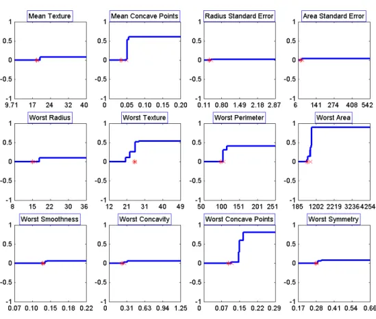
To fix ideas, let us consider, for instance, the Wisconsin Breast Cancer Database from the UCI Machine Learning Repository, [28], with data from cancer diagnosis. Each individual has 30 predictor variables, which, in principle, are to be taken into consideration. However, if we use BSVM, it turns out that only some of these predictor variables are shown to be relevant for the classification. In particular, with a specific choice of the parameter in our model, only 12 have at least one non-zeroω`b,and are thus those which need to be taken into account. Tables
1 and 2 focus on two of these relevant predictor variables, namelyMean Concave PointsandWorst Radius. For instance, for predictor variable Mean Concave Points and cutoff b = 0.0514, the weight is 0.514. For predictor variableWorst Radius, the only cutoff is b= 17.72,and has a weight of 0.1006. Since the output of the features proposed in this paper is always binary, the importance represented by the coefficient is always measured in the same scale. This means that havingMean Concave Pointsgreater than or equal to 0.0514 is more important for the classification than havingWorst Radiusgreater than or equal to 17.72. Moreover, for predictor variableWorst Radius, the only important issue for classification purposes is whether this variable takes a value greater than or equal to its unique critical value, namely, 17.72. In contrast, for variableMean Concave Points other cutoffs are also used in the classifier.
2.2
Visualization tool
The weightω`b gives insightful knowledge about how predictor variable`together with the cutoffbinfluences the
b ω`b
0.0492 0.0279 0.0514 0.5140 0.0559 0.0615
Table 1: Cutoffs and weights for predictor variableMean Concave Points.
b ω`b
17.720 0.1006
Table 2: Cutoffs and weights for predictor variableWorst Radius.
cutoff.
The role of predictor variable`in the score function is modeled by the stepwise function
s7→ X
{b∈B`|s≥b}
ω`b. (4)
This stepwise function is useful since it approximates the most adequate mapping to be applied to predictor variable
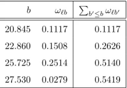
`to optimize the classification task. As an illustration, Table 3 shows, for predictor variable Worst Texture, its cutoffsb,the corresponding weightsω`b and the cumulative weightsPb0≤bω`b0.
b ω`b Pb0≤bω`b0
20.845 0.1117 0.1117 22.860 0.1508 0.2626 25.725 0.2514 0.5140 27.530 0.0279 0.5419
Table 3: Weights and cumulative weights for predictor variableWorst Texture.
We propose a plot of function (4) in order to gain insight about the contribution of predictor variable `to the classifier. This plot is a valuable tool to practitioners, who can use it to interpret the classifier, describing the role every predictor variable plays in the classification. In particular, it allows a direct choice of the relevant predictor variables, and detection of critical values and intervals.
contribution to the score function. Predictor variables Mean Concave Points, Worst Area and Worst Concave Pointsare the most important, whereasWorst TextureandWorst Perimeterhave a medium importance. Using this graphical representation, in predictor variableMean Concave Points, we can detect a critical value which, as said in the previous section, is at point 0.0514. In the case ofWorst Texture, in the interval between 21 and 27 the importance of this predictor variable grows up little by little, whereas outside this interval it remains constant. We can say that in this case we have a critical interval instead of a critical cutoff.
We have also plotted in Figure 1 the median (represented by a star) and the mean (represented by a cross). It can be seen how, although the mean or the median are sometimes a good choice for the cutoff, this does not happen in general, and BSVM prefers other choices.
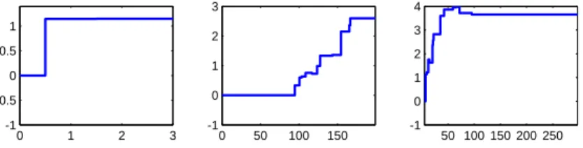
Graphical representations like Figure 1 can provide insight into the role a predictor variable plays in the classifier. In Figure 2, we present three different scenarios, found by applying the proposed method to other publicly available databases. More details can be found in Section 4. In the first case, there is just one value which is critical for classification. The second instance suggests an S-shaped transformation, similar toWorst Texturein Figure 1; it identifies a critical interval, within which the behavior is linear. Other types of mappings, harder to interpret, are, of course, possible. This is the case of the third function, which suggests a logarithmic transformation.
0 1 2 3 -1 -0.5 0 0.5 1 0 50 100 150 -1 0 1 2 3 50 100 150 200 250 -1 0 1 2 3 4
Figure 2: Transformations suggested by the method
Summing up, we have proposed a classifier that, using simple queries of type (1), allows us to visualize the role every predictor variable plays in the classification. Now, it is time to describe the procedure for finding the weights
ω`b associated to each predictor variable and cutoff. We follow an SVM-based framework, developed in the next
section.
2.3
Support vector machines
In order to chooseωandβ we follow an SVM-based approach which consists in finding the separating hyperplane which maximizes the margin in the feature space, i.e. the space of the images Φ(xu) of the objects u in the
training sampleI.The use of margin maximization is theoretically motivated by the bounds on the generalization ability [31, 34, 35], where the probability of misclassifying a forthcoming individual is bounded by a function which is decreasing in the margin. The so-calledhard-margin SVM approach proposes the choice of the separating hyperplane with maximal margin, i.e. the hyperplane which correctly classifies all objects inIand is furthest from the closest object. In contrast, the so-calledsoft-margin approach, allows some objects to be misclassified. We use
this latter version as it has been empirically shown to avoid overfitting, a phenomenon which happens when a low misclassification rate inI does not generalize to forthcoming objects. The soft-margin maximization problem is formulated in this paper by
min kωk+CP u∈Iξ u s.t.: cu ω>Φ(xu) +β +ξu≥1 ∀u∈I ξu≥0 ∀u∈I ω∈IRN, β∈IR, (5)
where the decision variables are the weight vectorω,the threshold value β and perturbations ξu associated with
the misclassification of objectu∈I.k · k denotes the L1 norm,C is a constant that trades off the margin in the correctly classified objects and the perturbationsξu,andN=Pp
`=1](B`),where](S) denotes the cardinality of a
setS.
An appropriate value ofC is chosen here, as detailed in Section 4.1, by inspecting a wide range of values and then measuring the performance with respect to misclassification rates, assessed by cross-validation, [23].
SVM seeks the separating hyperplane maximizing a function of the distances. There are many different possible choices for the distance function, which lead to different variants of SVM, [9]. Whereas the distance between points has usually been considered in the literature as the Euclidean norm, yielding the margin to be measured by the Euclidean norm as well, other norms such as theL1norm and theL∞norm have been considered and successfully
applied. See for instance [5, 7, 10, 24, 25, 32, 36] and the references therein. Moreover, the choice of theL∞ norm
to measure distances is equivalent to the use of theL1 norm regularization, also called lasso penalty, [21, 33]. Contrary to the Euclidean case, in which a maximal margin hyperplane can be found by solving a quadratic program with linear constraints, if, as in this paper, theL1 norm regularization is used, then an optimal solution of the corresponding optimization problem can be found by solving a Linear Programming (LP) problem. In [30], empirical results show that “in terms of separation performance,L1,L∞ and Euclidean norm-based SVM tend to
be quite similar”. Moreover, theL1 norm regularization contributes to sparsity in the classifier, yieldingω with many components equal to zero, see for instance [7, 15] or [26], which states that “one of the principal advantages of 1-norm support vector machines (SVMs) is that, unlike conventional 2-norm SVMs, they are very effective in
reducing input space features for linear kernels”.
Sincek · kis theL1 norm, Problem (5) can be formulated as the following LP problem,
min Pp `=1 P b∈B`(ω + `b+ω − `b) +C P u∈Iξ u s.t.: Pp `=1 P b∈B`(ω + `b−ω − `b)c uφ `b(xu) +βcu+ξu≥1 ∀u∈I ω+`b≥0 ∀b∈B`,∀`= 1,2, . . . , p ω−`b≥0 ∀b∈B`,∀`= 1,2, . . . , p ξu≥0 ∀u∈I β ∈IR. (6)
After finding the maximal margin hyperplane in the feature space defined byF,the score function has the form described in (3).
As said before, for each feature, the absolute value of its coefficient indicates the importance of that feature for the classification. In particular, features whose corresponding coefficient is zero can be seen as irrelevant for classification purposes. Using basic Linear Programming theory, it is easy to see that the number of features with non-zero coefficient is not larger than the number of objects in the training sample.
3
Column Generation
Problem (6) is a large scale linear program, which may be solved by any method which can handle SVM with the
L1 norm regularization, including general-purpose LP procedures or more ad-hoc methods, see e.g. [15]. In this paper, we propose Problem (6) to be solved by the well-known Mathematical Programming tool called Column Generation, initially introduced for the cutting-stock problem [17], and successfully used, under different variants, in different works on Support Vector Machines, such as [6, 8, 14, 26]. A brief discussion on how Column Generation is tailored to solve Problem (6) follows.
Instead of solving directly Problem (6), which has a high number of decision variables, the Column Generation technique solves a series of reduced problems where decision variables, corresponding to features in the setF,are iteratively added as needed.
ForF ⊂ F,let Master Problem (6-F) be Problem (6) with the family of featuresF.In each iteration, we first solve Problem (6-F). The next step is to check whether the current solution is optimal for Problem (6) or not, and, in the latter case, generate a new featureφimproving the objective value of the current solution. The generated feature is added to the family of featuresF.This process is repeated until optimality is reached.
To generate new features, we use the dual formulation of Problem (6),
max P u∈Iλu s.t.: −1≤P u∈Iλucuφ(xu)≤1 ∀φ∈ F P u∈Iλucu= 0 0≤λu≤C u∈I. (7)
The dual formulation of the Master Problem (6-F) only differs from this one in the first set of constraints, which should be attained∀φ∈F instead of∀φ∈ F.
Let (ω∗, β∗) be an optimal solution of Master Problem (6-F), and let (λ∗u)u∈I be the values of the corresponding
optimal dual solution. If the optimal solution of the Master Problem (6-F) is also optimal for Problem (6), then, for every featureφ∈ F the constraints of the Dual Problem (7) will hold, i.e.
−1≤X
u∈I
λ∗ucuφ(xu)≤1. (8)
Denote Γ(φ) =P
u∈Iλ∗ucuφ(xu).If (ω∗, β∗) is not optimal for Problem (6), then the most violated constraint gives
us information about which feature is promising and could be added toF,in the sense that adding such a feature to the set F would yield, at that iteration, the highest improvement of the objective function. Thus, we wish to generate a new featureφ∈ F maximizing|Γ(φ)|.
In the remainder of this Section we give a more detailed description of our implementation of the Column Generation algorithm.
3.1
Initial set of features
In the column generation procedure new features are sequentially added to the problem, based on the dual values of the current solution. The Column Generation technique starts with an initial Master Problem, i.e. a set of features
F0 must be chosen to initialize the algorithm. We have chosen to start with one feature per predictor variable, with the cutoff set equal to its median in the objects ofI.
3.2
Generation of features
Finding the bestφ∈ F reduces to finding a predictor variable`and a cutoff b∈B`,such that |Γ(φ`b)|, withφ`b
defined by (2), is maximal. This can be done by full inspection of the set{φ`b+ `
, φ`b− `
: `= 1,2, . . . , p},where, for each predictor variable`,the cutoffb+` (respectivelyb−`) is the value inB` for which Γ(φ`b) is highest (respectively
lowest). In this section we describe an algorithm for, fixed the predictor variable`,finding the cutoffb+` maximizing
Γ(φ`b).Findingb−` can be done in a similar way.
First, we sort all the objects in decreasing order by the values of the predictor variable`. Denote byu(i) the object ini-th position. For simplicity, suppose there are not repeated values, i.e. xu`(1) > x`u(2) > . . . > xu`(](I)).
The case with repeated values will be analyzed later.
Once ` is fixed and all the objects are sorted by the values of the predictor variable `, the value Γ(φ`b) can
be efficiently calculated with a recursive procedure. Indeed, for certain i∈ {1,2, . . . , ](I)}, we have Γ(φ`bi+1) = Γ(φ`bi) +λ
∗ u(i+1)c
u(i+1), whereb
i denotes the cutoff chosen as x
u(i)+xu(i+1)
2 .Moreover, sinceλ
∗
u is nonnegative for
allu∈I,we have that Γ(φ`bi+1)≥Γ(φ`bi) whenever c
u(i+1) = 1. Hence, checking whether φ
`bi is a maximum is
not needed for everyi, but only for thoseisuch thatcu(i)= 1 andcu(i+1)=−1.
In the case in which there are repeated values in{xu` : u∈I}, the rule above does not apply. Let iand tbe such thatxu`(i−1) > x`u(i) =xu`(i+1) =. . . =xu`(i+t) > x`u(i+t+1).Note that, in the set of objects where predictor
variable` has the same value, there could be objects belonging to different classes. In this case, the value b=bi
must be checked, whatever the value ofcu(i+t+1). However, ifcu(i)=cu(i+1)=. . .=cu(i+t) andcu(i+t+1) = 1 we
know that settingb =bj, for anyj =i, i+ 1, . . . , i+t,will be improved by setting b =bi+t+1.This means that
b=bi does not give a maximum of Γ(φ`b).Only ifcu(i)= 1 andcu(i+t+1)=−1, it is worth to considerb=bi as a
candidate to be the maximum.
The minimization of Γ is done analogously. For example, in case of no repeated values, candidates to be a minimum correspond to objectsu(i) belonging to class−1 where the next objectu(i+ 1) belongs to class 1.
Taking into account all these considerations we obtain, for a fixed predictor variable `, given the dual values
λ∗u,the algorithm described below, which finds the cutoffb
+ ` (and respectively,b − `) for which Γ(φ`b+ `) (respectively, Γ(φ`b−
` )) is maximal (respectively, minimal).
Algorithm 1: Choosing two cutoffs for predictor variable`.
Step 0. Sort the objects decreasingly by x`:x u(i)
` .
Step 1. Seti←1,sum←0,max←0,min←0,i+←iandi− ←i.
Step 2. Setsum←sum+λ∗u(i)cu(i).
Step 3. Step 3.1. Ifxu`(i)=xu`(i+1),then, go to Step 4.
Step 3.2. Otherwise, if for somet >0, xu`(i−t−1)< x`u(i−t)=. . .=x`u(i)< xu`(i)−1 and there existsj
withj= 1, . . . , tandcu(i)6=cu(i−j),then:
• Ifsum>max, then setmax ←sum andi+←i. • Ifsum<min, then setmin ←sum andi−←i.
Step 3.3. Otherwise,
• ifcu(i)= 1, cu(i+1)=−1 andsum>max, then setmax ←sum andi+←i. • ifcu(i)=−1, cu(i+1)= 1 andsum<min, then setmin ←sum andi−←i.
Step 4. Seti←i+ 1.Ifi≤](I),then go to Step 2. Otherwise STOP:b+` =bi+ andb−` =bi−.
We may notice that Step 0 can be performed in a preprocessing stage, of running time O(|I|log(|I|)), for all calls to Algorithm 1 for predictor variable`. Hence, considering such sorting as preprocessing, it follows that each call to Algorithm 1 runs in O(|I|) time, since Step 3 is performed at most once for each object in the training sample, while the calculations involved in this step can be performed in constant time.
3.3
Implementation details
The column generation algorithm has been implemented as follows. The initial set of features F0 is built, as described in Section 3.1, using features whose cutoffs are the medians of the predictor variables. Then, Problem
(6-F0) is solved for such initial set of features. The dual values of the optimal solution found, are used to generate new features.
In every step of the column generation algorithm, instead of generating just one feature (the one maximizing |Γ(φ)|), we generate two features for every predictor variable `, given by the cutoffs b`+, b−` for which Γ(φ`b) is
respectively maximal and minimal. This is done using Algorithm 1, as described in Section 3.2. We do it for all the predictor variables, thus obtaining 2pfeatures. Those generated features having |Γ(φ)| >1 are added to F
and the LP problem (6-F) is solved. These steps are repeated until all the generated features have |Γ(φ)| ≤1,in which case, we have found an optimal solution of Problem (6). A summary of this Column Generation Algorithm is described as follows.
Algorithm for Column Generation.
Step 0. Set F0 ← {φ1b∗
1, φ2b∗2, . . . , φpb∗p}, whereb
∗
` is the median of the predictor variable`, for `= 1,2, . . . , p.
SetF ←F0.
Step 1. Solve Problem (6-F). Let (ω∗, β∗) be its optimal solution, with dual valuesλ∗u,∀u∈I.
Step 2. For each `= 1,2, . . . , pdo:
Step 2.1. RunAlgorithm 1to chooseb+` and b−`.
Step 2.2. If Γ(φ`b+ ` )>1,then setF ←F∪ {φ`b+ ` }. Step 2.3. If Γ(φ`b− ` )<−1,then setF ←F∪ {φ`b− ` }.
Step 3. If F has been modified, then go to Step 1, otherwise STOP: we have found an optimal solution of Problem (6).
In Step 1, we need to solve the LP problem (6-F). In our numerical results we have used CPLEX 8.1.0 as the LP solver.
Our numerical experience shows that the number of features used by our classifier, i.e., the ones that have been generated by the BSVM and have non-zero coefficient in the classifier, is usually rather large. In order to obtain
a more simple classifier, we proceed with a wrapper feature selection procedure in which features are recursively deleted. In this procedure, which has been successfully applied in standard SVM, see [18], all the generated features with zero coefficient in the classifier as well as the feature with non-zero coefficient having the smallest absolute value are eliminated. Then, the coefficients are recomputed by the optimization of the Problem (6). This elimination procedure is repeated until the number of features with non-zero coefficient is below a number given in advance.
As reported in our numerical experience in Section 4.5, this procedure typically allows one to reduce the number of features used in the classifier at the expense of a mild loss in the classification ability.
4
Numerical results
4.1
Databases, benchmarking methods and accuracy measure
In this section we illustrate the classification ability as well as the most desirable properties of BSVM. With this aim, a series of numerical experiments has been performed using databases publicly available from the UCI Machine Learning Repository [28]. Nine different databases were used, namely, the Sonar Database, called here
sonar; the Cylinder Bands Database, called herebands; the Credit Screening Database, called here credit; the Ionosphere Database, called hereionosphere; the New Diagnostic Database, contained in the Wisconsin Breast Cancer Databases, called herewdbc; the Cleveland Clinic Foundation Database, called herecleveland; the Boston Housing Database, called here housing; the Pima Indians Diabetes Database, called here pima; and the BUPA Liver-disorders Database, called herebupa.
In case of existence of missing values, as occurs for instance inbandsandcredit, objects with missing values were removed from the database. In databases such asbands andcredit, some of the predictor variables were nominal. Each of these predictor variables has been replaced by a set of binary variables in the following way: for every possible value ˆxof the original nominal predictor variable`, a new binary variable is built taking value one whenx`is equal to ˆxand zero otherwise. Thehousingdatabase is a typical regression dataset, but it is often used
for each database, the final number of objects and the number of predictor variables (all quantitative) can be found in the second column of each table.
All databases used are of small/moderate size. Very large datasets do not seem to be so suitable for a crude implementation of BSVM, since column generation methods are known to be time-consuming. In practice, for databases of much larger size than those used in these experiments, it might be convenient to either select a subsample of data with manageable size, or perform some dimensionality reduction technique such as Principal Component Analysis to obtain an appropriate number of variables.
In order to compare the BSVM classifier with other classifiers, we have tested the performance of three different benchmarking methods: Classification Trees, both with pruning (TreePr) and without pruning (TreeCr), linear SVM and a benchmarking method for the SVM with theL1norm regularization, namely, the NLPSVM proposed by Fung and Mangasarian in [15]. The classification accuracy of each method is measured by the leave-one-out correctness, as done in [15]. Below we give a brief description of this measure.
In the leave-one-out correctness, in what followslooc,for each object, the training sample is equal to the whole database except for this object, while the testing sample is equal to the excluded object. For each training sample, we construct a classifier which will be applied in the corresponding testing sample, returning a 1 if the only object in the testing sample is correctly classified and 0 otherwise. The looc is equal to the percentage of correctly classified objects. Since looc uses all but one object to build the classifier, the provided classification can be expected to be close to the one of the classifier trained with the complete dataset.
Given a training sample, it remains to specify the way the SVM as well as the BSVM classifiers are constructed. Problem (6), as well as the corresponding optimization problem for the linear SVM, contains a parameter that needs to be tuned, namely, the regularization parameterCwhich trades off misclassification errors in the training sample with the generalization error. As in [15], we limit the values of this parameter to the values 2i with
i=−12,−11, . . . ,12. ParameterC is then chosen so that it minimizes the misclassification rate after performing
10-fold cross-validation in the training data (which, as said before contains all but one object.) It has been empirically observed, e.g. [7, 11, 15], that the choice of the parameter C may strongly influence the number of features selected. Hence, one might have also chosenCby balancing misclassification rates and number of features
selected.
4.2
Classification ability
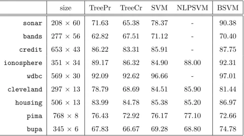
In Table 4 we report the looc of both Classification Trees, with and without pruning, linear SVM with normalized data, NLPSVM and BSVM. Note that for NLPSVM we only have results on five databases, the ones reported by Fung and Mangasarian [15] in their paper. From Table 4, we can see that BSVM outperforms the three benchmarking methods in six out of the nine databases we consider in this paper. This happens in theionosphere, thehousingand thebupadatabases. For the sonar,credit andwdbcdatabases, Fung and Mangasarian [15] do not report any results, but BSVM outperforms Classification Trees and linear SVM. In these six databases, the increase in accuracy of BSVM with respect to the best reported accuracy, ranges from 0.35% for thewdbcdatabase up to 12.01% for thesonardatabase. For the bandsdatabase, we are able to outperform Classification Trees, but not the linear SVM, which has an accuracy of 71.12% while we have 70.40%. Similarly, for theclevelanddatabase, we are able to outperform Classification Trees, but linear SVM and NLPSVM have a better classification accuracy, 84.51% and 85.90% respectively, while the one of BSVM is 81.44%. For thepimadatabase, BSVM underperforms the rest of the methods, where the decrease in accuracy of BSVM with respect to the best reported accuracy is equal to 4.44%. As a summary, we conclude that BSVM can be seen as a CART-like method (which may very good for practitioners, since relevant predictor variables and critical values of them are identified), with a classification power which is at least comparable, and in some cases much better than competing benchmarking techniques such as CART or other versions of SVM.
4.3
Interpretability
Classification Trees are widely used in applied fields as diverse as Medicine (diagnosis), Computer Science (data structures), Botany (classification), and Psychology (decision theory), mainly because they are easy to interpret. Therefore, high accuracy is not the only desirable property of a classifier, but also its interpretability. BSVM improves largely the interpretability of standard SVMs by the use of queries of type (1). In this section we illustrate how our method takes us one step further towards interpretability via the use of the visualization tool
size TreePr TreeCr SVM NLPSVM BSVM sonar 208×60 71.63 65.38 78.37 - 90.38 bands 277×56 62.82 67.51 71.12 - 70.40 credit 653×43 86.22 83.31 85.91 - 87.75 ionosphere 351×34 89.17 86.32 84.90 88.00 92.31 wdbc 569×30 92.09 92.62 96.66 - 97.01 cleveland 297×13 78.79 68.69 84.51 85.90 81.44 housing 506×13 83.99 84.78 85.38 85.20 86.97 pima 768×8 76.43 72.92 76.17 77.10 72.66 bupa 345×6 67.83 66.67 69.28 68.80 74.78
Table 4: Looc for BSVM and benchmarking methods
proposed in Section 2.2.
To do this, we have considered two databases with different characteristics, namelybupaandsonar, which have respectively 6 and 60 predictor variables. Since the focus here is on interpretability, and not generalization ability, the whole database have been used to build the classifier. ParameterC has been chosen by 10-fold cross-validation in the whole database.
If SVM is performed,bupa uses all 6 predictor variables, i.e., all predictor variables have associated a non-zero weight. BSVM uses all 6 predictor variables as well, where we say that a predictor variable has been used if there exists at least one feature associated to this predictor variable which has a non-zero coefficient in the classifier. The total number of features used by BSVM is 62.
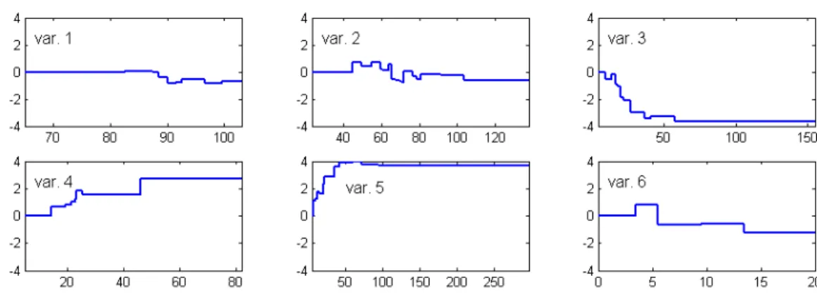
A quick look at Figure 3, with information from bupa, allows us to say that predictor variables 3, 4 and 5 have the strongest influence in the classifier. It is particularly simple to analyze from the picture the influence of predictor variable 3. Indeed, we can see that predictor variable 3 presents an S-shaped form, with a linear behavior within the interval with endpoints 0 and 25 and constant outside. Moreover, the slopes are negative, meaning that, the higher the value of the predictor variable (up to 25), the stronger the tendency to be classified in the negative class. On top of that, we see that whether predictor variable 3 takes a value of, say, 25, or, instead, a much higher value, turns out to be irrelevant for classification purposes.
A similar behavior is detected for predictor variable 4. From 0 to 25, the influence is linear, but after that is stable and finally jumps around value 45. Now the slopes are positive, implying that, the higher the value of predictor variable 4, the stronger the tendency to be classified in the positive class.
Predictor variable 5 shows a logarithmic behavior, again with positive slopes and one critical value after which the function remains almost constant.
Figure 3: Graphical representation forbupa
In general, this example shows that the presence of many cutoffs, as in predictor variables 3, 4 and 5, is not an inconvenience for interpreting the classifier, whose behavior is easily detected via the visualization tool proposed.
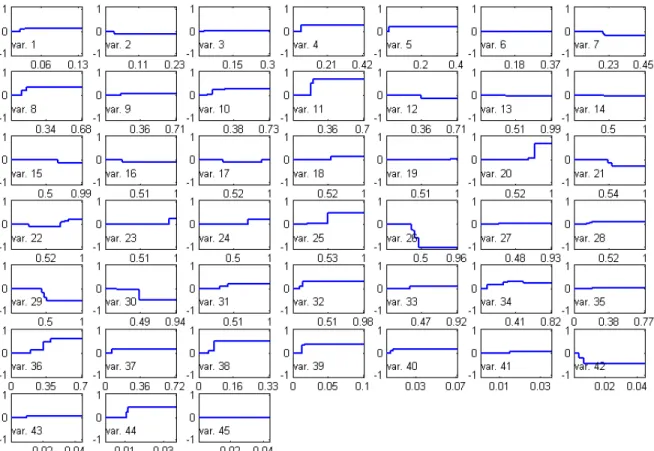
Now, take the example of databasesonar, which has 60 predictor variables. If SVM is performed, all 60 are used again, whereas BSVM uses 98 features, involving 45 different predictor variables. Hence, BSVM is able to make feature selection (it is able to detect as irrelevant for classification 25% of the predictor variables) in a database where linear SVM would consider all variables as relevant.
In Figure 4 the 45 used predictor variables are shown, renumbered for convenience. A simple look to this figure indicates that there are only four out of the 45 predictor variables with strong influence in the classifier, namely predictor variables 11, 20, 26 and 36. Predictor variables in positions 11 and 20 have just one main critical value, whereas predictor variables 26 and 36 present an almost linear behavior in a clearly identified interval.
We see again that the use of BSVM allows us to choose the relevant predictor variables, interpret the way such variables influence the classifier, and detect the critical values and intervals for each predictor variable.
4.4
Size of the BSVM classifier
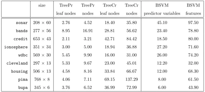
Simplicity in the classifier is another desirable property for practitioners. Because both BSVM and Classification Trees are based on simple queries of type (1), the size of the resulting classifier is a good proxy for their complexity. In Table 5, we compare the size of the classifiers constructed by BSVM and Classification Trees. We report average results over all the objects, i.e., over all the testing samples.
For both Classification Trees, with and without pruning, we report the total number of nodes in the final tree as well as the number of leaf nodes. For the BSVM classifier, we report the number of used predictor variables as well as the number of used features.
In our opinion, the fairest comparison for the complexity is to measure the number of nodes generated by Classification Trees against the number of features used by BSVM. As the results show, the size of the Classification Tree with pruning is always smaller. For the Classification Tree without pruning, in four out of the nine databases, namelycredit,cleveland,pimaandbupa, BSVM is smaller in size, while in a fifth one,housing, both classifiers are of similar size. This result in complexity for BSVM should be balanced with its better classification ability. From Table 4, BSVM outperforms Classification Trees with pruning except for thepimadatabase, with an increase in accuracy which ranges from 1.53% for thecredit database up to 18.75% for the sonar database. Similarly, BSVM outperforms Classification Trees without pruning except for thepimadatabase in which both methods have basically the same accuracy. The increase in accuracy of BSVM ranges from 2.19% for thehousingdatabase up to 25.00% for thesonardatabase.
size TreePr TreePr TreeCr TreeCr BSVM BSVM leaf nodes nodes leaf nodes nodes predictor variables features
sonar 208×60 2.76 4.52 18.40 35.80 45.10 97.50 bands 277×56 8.95 16.91 28.81 56.62 23.40 78.80 credit 653×43 2.11 3.21 42.71 84.42 18.50 80.00 ionosphere 351×34 3.00 5.00 18.94 36.88 27.20 71.60 wdbc 569×30 5.45 9.90 16.00 31.00 26.00 74.20 cleveland 297×13 5.33 9.67 23.00 45.01 12.20 32.00 housing 506×13 4.58 8.16 33.84 66.67 12.00 68.30 pima 768 ×8 4.06 7.11 69.15 137.29 8.00 61.50 bupa 345 ×6 3.76 6.52 36.99 72.99 6.00 43.90
Table 5: Size of benchmarking classifiers
of its classification ability, at the expense of a higher complexity of the classifier, which is comparable to the complexity of Classification Trees if no pruning is performed.
4.5
Reducing the number of used features
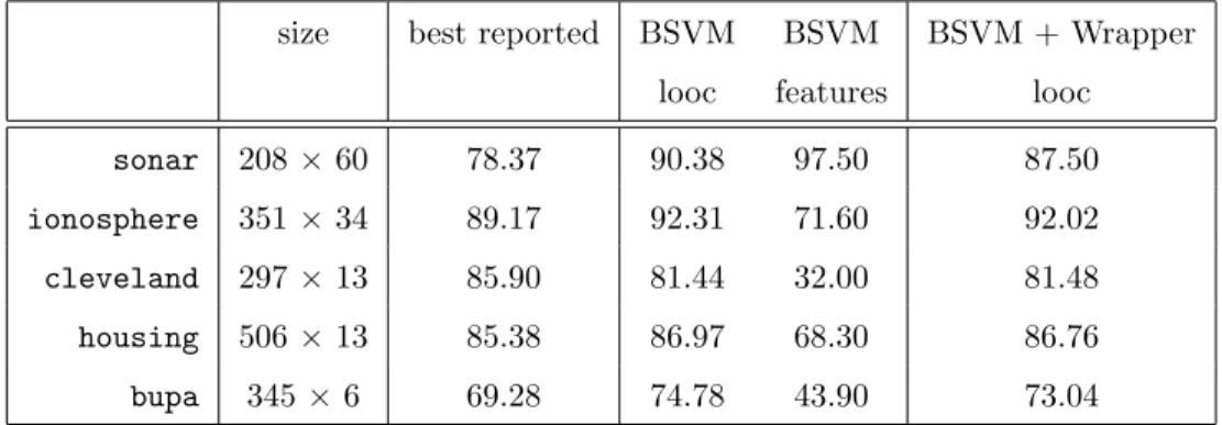
The complexity of the classifiers obtained by BSVM is usually high because a high number of features may be present in the rule, as we have discussed in the previous section. With the aim of reducing the complexity of the classifier obtained by our procedure, we have performed several experiments implementing the wrapping procedure described in Section 3.3. Due to computational burden, we present results on five databases. The selection of the databases has been done based on the running times, and it does not affect our conclusions. In Table 6 results on databasessonar,ionosphere,cleveland,housingandbupaare shown.
For convenience, we repeat some of the results already given in previous tables. The third and fourth columns report the best accuracy among all three benchmarking methods as well as the one of BSVM (when no wrapper procedure is applied), both processed from the data in Table 4. The fifth column contains the size (measured as number of used features) of the BSVM classifier, obtained from Table 5. The sixth column reports the accuracy of BSVM when the size of the classifier is reduced up to a maximum of 30 features. From those results we can
conclude that the classification ability of BSVM slightly deteriorates. More specifically, theclevelanddatabase, which was one in which the linear SVM outperformed BSVM, has essentially the same accuracy as before. This is not surprising, since the average number of features used by BSVM is equal to 32, as reported in Table 5. For theionosphereand thehousingdatabases, the looc remains almost the same, and therefore, BSVM outperforms the best of the three benchmarking methods while using at most 30 features. In thebupa database, the decrease in accuracy is equal to 1.74%, but even after this deterioration, BSVM with wrapping procedure still gives us the best accuracy. The conclusions for the sonar database are similar. Thus, even with this limit on the number of features, BSVM is still able to outperform the three benchmarking methods, except for the case of thecleveland
database in which, as happens without wrapping, BSVM is outperformed by the linear SVM and the NLPSVM. We decided to further investigate those databases in which the wrapping of the BSVM classifiers did not affect the accuracy, namely thecleveland,ionosphereandhousingdatabases. In thehousingdatabase, the wrapped BSVM classifier, as said above, has the best accuracy, while its size is half of that from the tree without pruning (which is the best of the two trees in terms of accuracy). For cleveland and ionosphere, the size was not competitive enough. Therefore, we further reduced the number of used features to a maximum of 20. The looc ofcleveland andionosphere was exactly the same as the one obtained when the number of used features was limited to 30. This is specially remarkable for the ionosphere database, in which we can reduce the number of features to less than a third, from 71.60 to at most 20, while the accuracy decreases only by 0.29%.
size best reported BSVM BSVM BSVM + Wrapper looc features looc
sonar 208 ×60 78.37 90.38 97.50 87.50
ionosphere 351 ×34 89.17 92.31 71.60 92.02
cleveland 297 ×13 85.90 81.44 32.00 81.48
housing 506 ×13 85.38 86.97 68.30 86.76
bupa 345×6 69.28 74.78 43.90 73.04
4.6
Presence of outliers
The classifier proposed in this paper is based on threshold functions, thus it seems that extreme observations, with very high or very low values, will not have a strong influence in the classifier. To empirically test this conjecture, a series of experiments has been performed where some outliers were artificially introduced. Every cell in the database was chosen to be an outlier with probability 0.05. Those cells chosen were modified by adding ρtimes the range of its predictor variable in the training sample. We present here results forρ= 10.For other values ofρ
we obtained similar results, and therefore are not reported.
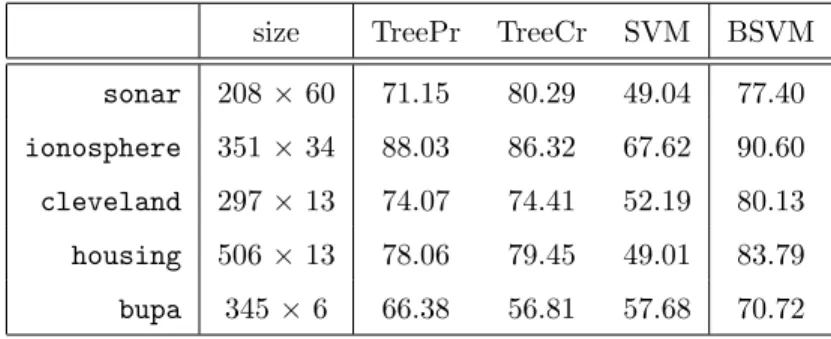
As in Section 4.5, and again due to computational burden, we present results on five databases. In Table 7 results on databasessonar, ionosphere,cleveland, housingand bupa are shown. We compare BSVM against Classification Trees and linear SVM. We do not report results on the NLPSVM since outliers are not discussed in the paper of Fung and Mangasarian [15]. The classification ability of the linear SVM classifier dramatically worsens when introducing outliers, and clearly underperforms the other two methods. Classification Trees and BSVM are only slightly affected. We outperform Classification Trees in all databases exceptingsonar. Therefore, our conjecture is supported.
size TreePr TreeCr SVM BSVM
sonar 208×60 71.15 80.29 49.04 77.40
ionosphere 351×34 88.03 86.32 67.62 90.60
cleveland 297×13 74.07 74.41 52.19 80.13
housing 506×13 78.06 79.45 49.01 83.79
bupa 345 ×6 66.38 56.81 57.68 70.72
Table 7: Looc for BSVM and benchmarking methods. Databases with outliers
5
Conclusions and further research
In this paper a new SVM-based tool for supervised classification has been proposed. The classifier gives insightful knowledge about the way the predictor variables influence the classification. Indeed, the nonlinear behavior of the
data is modeled by the BSVM classifier using simple queries, of type (1), easily interpretable by practitioners. In terms of generalization ability, BSVM is competitive against Classification Trees and SVM, since it has a higher leave-one-out correctness in most databases tested. Moreover, by its nature, BSVM is an interesting tool when a good classification ability is required, but also interpretability of the results is an important issue. Indeed, even though the crude BSVM may yield a large set of features with non-zero coefficients, we have shown that interpretability might also be possible in this situation, and we can use a graphical method for getting insight about the role each predictor variable plays in the classifier. If needed, a wrapping procedure enables one to keep the number of features used at a desired level, at the expense of a slight deterioration in the classification ability.
Concerning to robustness, some numerical tests have been performed to analyze how the classification ability (slightly) deteriorates when outliers exist. We can conclude from the results that BSVM is much more robust than linear SVM against outliers.
Several issues analyzed in this paper may deserve further study. For instance, the setsB`contain, by definition,
all midpoints among consecutive values of each predictor variable in the training sample. An adequate filtering in a pre-processing step would reduce the computational burden, specially for large datasets, and might help to reduce the overfitting a very complex model may produce.
The binarization procedure has been applied to each predictor variable separately. If interactions between predictor variables are expected to be relevant, more general binarization procedures might be considered. These issues, as well as the extension to Support Vector Regression, will be addressed in the next future.
Acknowledgements
The authors thank the two anonymous referees and the associate editor for their helpful comments to improve both the exposition as well as the numerical results in Section 4. The authors are grateful to Jingbo Wang and Rafael Blanquero for the support they have offered to obtain some of the results in Section 4.
References
[1] R. Andrews, J. Diederich, and A.B. Tickle. A survey and critique of techniques for extracting rules from trained artificial neural networks. Knowledge Based Systems, 8:373–389, 1995.
[2] B. Baesens, R. Setiono, C. Mues, and J. Vanthienen. Using neural network rule extraction and decision tables for credit-risk evaluation. Management Science, 49:312–329, 2003.
[3] N. Barakat and J. Diederich. Learning-based rule-extraction from support vector machines. In14th Interna-tional Conference on Computer Theory and Applications ICCTA 2004, 2004.
[4] N. Barakat and J. Diederich. Eclectic rule-extraction from support vector machines. International Journal of Computational Intelligence, 2(1), 2005.
[5] K. Bennett. Combining support vector and mathematical programming methods for induction. In B. Sch¨olkopf, C. Burges, and A. Smola, editors,Advances in Kernel Methods: Support Vector Learning, pages 307–326. MIT Press, 1999.
[6] J. Bi, T. Zhang, and K.P. Bennett. Column-generation boosting methods for mixture of kernels. InProceedings of the Tenth ACM SIGKDD International Conference on Knowledge Discovery and Data Mining, pages 521– 526, 2004.
[7] P. S. Bradley and O. L. Mangasarian. Feature selection via concave minimization and support vector machines. InMachine Learning Proceedings of the Fifteenth International Conference(ICML ’98), pages 82–90. Morgan Kaufmann, 1998.
[8] P.S. Bradley and O.L. Mangasarian. Massive data discrimination via linear support vector machines. Opti-mization Methods and Software, 13:1–10, 2000.
[9] E. Carrizosa. Data Mining and Mathematical Programming, volume 45 ofCRM Proceedings & Lecture Notes, chapter Support Vector Machines and Distance Minimization, pages 1–14. AMS and Centre de Recherches Math´ematiques., 2008.
[10] E. Carrizosa, B. Mart´ın-Barrag´an, and D. Romero Morales. Minimum-cost feature selection for classification: A biobjective model. Discrete Applied Mathematics, 156:950–966, 2008.
[11] F. Colas, P. Pacl´ık, J.N. Kok, and P. Brazdil. Does SVM really scale up to large bag of words feature spaces? In M.R. Berthold, J. Shawe-Taylor, and N. Lavrac, editors,Advances in Intelligent Data Analysis VII, Lecture Notes in Computer Science, 4723, pages 296–307. Springer, 2007.
[12] C. Cortes and V. Vapnik. Support-vector networks. Machine Learning, 20(3):273–297, 1995.
[13] M. Craven and J. Shavlik. Using neural networks for data mining. Future Generation Computer Systems, 13:211–229, 1997.
[14] A. Demiriz, K.P. Bennett, and J. Shawe-Taylor. Linear programming boosting via column generation.Machine Learning, 46(1):225–254, 2002.
[15] G. Fung and O.L. Mangasarian. A feature selection Newton method for support vector machine classification.
Computational Optimization and Applications, 28(2):185–202, 2004.
[16] G. Fung, S. Sandilya, and R. Bharat Rao. Rule extraction from linear support vector machines. InProceedings of the Eleventh ACM SIGKDD International Conference on Knowledge Discovery and Data Mining, pages 32–40, 2005.
[17] P.C. Gilmore and R.E. Gomory. A linear programming approach to the cutting-stock problem. Operations Research, 9:849–859, 1961.
[18] I. Guyon, J. Weston, S. Barnhill, and V. Vapnik. Gene selection for cancer classification using support vector machines. Machine Learning, 46:389–422, 2002.
[19] H. Hand, H. Mannila, and P. Smyth. Principles of Data Mining. MIT Press, 2001.
[20] T. Hastie and R. Tibshirani. Classification by pairwise coupling. The Annals of Statistics, 26(2):451–471, 1998.
[21] T. Hastie, R. Tibshirani, and J. Friedman.The Elements of Statistical Learning: Data Mining, Inference, and Prediction. Springer, New York, 2001.
[22] R. Herbrich. Learning Kernel Classifiers. Theory and Algorithms. MIT Press, 2002.
[23] R. Kohavi. A study of cross-validation and bootstrap for accuracy estimation and model selection. In Proceed-ings of the 14th International Joint Conference on Artificial Intelligence, pages 1137–1143. Morgan Kaufmann, 1995.
[24] O. L. Mangasarian. Generalized support vector machines. In A. Smola, P. Bartlett, B. Sch¨olkopf, and D. Schuurmans, editors,Advances in Large Margin Classifiers, pages 135–146. MIT Press, 2000.
[25] O.L. Mangasarian. Linear and nonlinear separation of patterns by linear programming. Operations Research, 13:444–452, 1965.
[26] O.L. Mangasarian and M.E. Thompson. Massive data classification via unconstrained support vector machines.
Journal of Optimization Theory and Applications, 113:315–325, 2006.
[27] D. Martens, B. Baesens, T. Van Gestel, and J. Vanthienen. Comprenhensible credit scoring models using rule extraction from support vector machines. European Journal of Operational Research, 183:1466–1476, 2007.
[28] D.J. Newman, S. Hettich, C.L. Blake, and C.J. Merz. UCI Repository of Machine Learning Databases. http://www.ics.uci.edu/∼mlearn/MLRepository.html, 1998. University of California, Irvine, Dept. of Infor-mation and Computer Sciences.
[29] H. N´u˜nez, C. Angulo, and A. Catal`a. Rule extraction from support vector machines. In Proceedings of the European Symposium on Artificial Networks, pages 107–112, 2002.
[30] J.P. Pedroso and N. Murata. Support vector machines with different norms: motivation, formulations and results. Pattern Recognition Letters, 22:1263–1272, 2001.
[31] J. Shawe-Taylor, P.L. Bartlett, R.C. Williamson, and M. Anthony. Structural risk minimization over data-dependent hierarchies. IEEE Transactions on Information Theory, 44(5):1926–1940, 1998.
[32] A. Smola, T.T. Friess, and B. Sch¨olkopf. Semiparametric support vector and linear programming machines. In M.J. Kearns, S.A. Solla, and D.A. Cohn, editors, Advances in Neural Information Processing Systems 10, pages 585–591. MIT Press, 1999.
[33] R. Tibshirani. Regression shrinkage and selection via the lasso.Journal of the Royal Statistical Society. Series B, 58(1):267–288, 1996.
[34] V. Vapnik. The Nature of Statistical Learning Theory. Springer-Verlag, 1995.
[35] V. Vapnik. Statistical Learning Theory. Wiley, 1998.
[36] J. Weston, A. Gammerman, M.O. Stitson, V. Vapnik, V. Vovk, and C. Watkins. Support vector density estimation. In B. Sch¨olkopf, C. Burges, and A. Smola, editors,Advances in Kernel Methods - Support Vector Learning, pages 293–305. MIT Press, 1999.