NBER WORKING PAPER SERIES
OPTIMAL MARKET TIMING Erica X. N. Li
Dmitry Livdan Lu Zhang Working Paper 12014
http://www.nber.org/papers/w12014
NATIONAL BUREAU OF ECONOMIC RESEARCH 1050 Massachusetts Avenue
Cambridge, MA 02138 January 2006
We thank Lubos Pastor, Leonid Kogan, and seminar participants at MIT for helpful discussions. The Matlab and C++ programs used for the scientific computation in this paper are available from the authors upon request. All remaining errors are our own. The views expressed herein are those of the author(s) and do not necessarily reflect the views of the National Bureau of Economic Research.
©2006 by Erica X. N. Li, Dmitry Livdan and Lu Zhang. All rights reserved. Short sections of text, not to exceed two paragraphs, may be quoted without explicit permission provided that full credit, including ©
Optimal Market Timing
Erica X. N. Li, Dmitry Livdan and Lu Zhang NBER Working Paper No. 12014
January 2006
JEL No. E13, E22, E32, E44, G12, G14, G24, G31, G32, G35 ABSTRACT
We use a fully-specified neoclassical model augmented with costly external equity as a laboratory to study the relations between stock returns and equity financing decisions. Simulations show that the model can simultaneously and in many cases quantitatively reproduce: procyclical equity issuance; the negative relation between aggregate equity share and future stock market returns; long-term underperformance following equity issuance and the positive relation of its magnitude with the volume of issuance; the mean-reverting behavior in the operating performance of issuing firms; and the positive long-term stock price drift of firms distributing cash and its positive relation with book-to-market. We conclude that systematic mispricing seems unnecessary to generate the return-related evidence often interpreted as behavioral underreaction to market timing.
Erica X. N. Li
Simon School of Business University of Rochester [email protected] Dmitry Livdan
Mays Business School Texas A&M University [email protected] Lu Zhang
William E. Simon Graduate School of Business Administration
University of Rochester Rochester, NY 14627 and NBER
1
Introduction
We study the dynamic, quantitative relations between stock returns and equity financing decisions using a fully-specified neoclassical model augmented with costly external equity.
The issue is important. Recent literature in empirical corporate finance has uncovered an array of evidence often interpreted as substantiating a window-of-opportunity theory of financing decisions in response to systematic mispricing in equity markets. In particular, Rit-ter (2003) argues that managers can create value for existing shareholders by timing financing decisions to take advantage of time-varying relative costs of debt and equity caused by market inefficiencies. Managers can issue equity when their stock prices are high and turn to internal funds or debt when stock prices are low. As supporting evidence, Ritter cites many empirical studies that document long-run abnormal returns following corporate financing events.
Using simulations, we demonstrate that our neoclassical model can reproduce simultane-ously, and in many cases quantitatively, many stylized facts often interpreted as behavioral market timing. These facts include: (i) the amount and frequency of equity issuance are pro-cyclical (e.g., Choe, Masulis, and Nanda (1993)); (ii) the new equity share in total amount of new equity and debt financing is a significantly negative predictor of aggregate stock market returns (e.g., Baker and Wurgler (2000)); (iii) firms conducting seasoned equity offerings underperform nonissuing firms with similar size and book-to-market in the long run, and the magnitude of this underperformance increases with the volume of issuance (e.g., Loughran and Ritter (1995), and Spiess and Afflect-Graves (1995)); (iv) the operating performance of issuing firms exhibits substantial improvements prior to the equity offerings, but then deteri-orates, and issuing firms are also disproportionately high-investing, high-growth firms (e.g., Loughran and Ritter (1997)); (v) there exists a positive long-term stock price drift for firms
distributing cash back to shareholders, and the magnitude of the drift is stronger among value firms (e.g., Lakonishok and Vermaelen (1990), Ikenberry, Lakonishok, and Vermaelen (1995), and Michaely, Thaler, and Womack (1995)); and finally (vi) capital investment is negatively associated with future stock returns in the cross section, and the magnitude of this association is stronger among firms with higher cash flows (e.g., Titman, Wei, and Xie (2004), Anderson and Garcia-Feij´oo (2005), Polk and Sapienza (2005), and Xing (2005)).
We deliberately do not include any behavioral bias in our model, in which firms choose investment and financing decisions optimally in response to aggregate and firm-specific productivity shocks. Firm-specific shocks affect corporate decisions through operating cash flows. And aggregate shocks affect corporate decisions through both operating cash flows and an exogenously-specified stochastic discount factor that admits a countercyclical price of risk, as in Berk, Green, and Naik (1999). Our simulations suggest that systematic mispricing seems unnecessary to generate the evidence often interpreted as behavioral underreaction to market timing, or more generally, the window-of-opportunity theory of financing decisions. However, investor sentiment, for example, as modeled by Barberis, Huang, and Santos (2001), can potentially affect the countercyclical price of risk exogenously specified in our model. We therefore do not suggest that the timing-related evidence is fully rational, but we do argue that investor sentiment seems unnecessary.
The intuition driving our results is simple. Controlling for expected productivity, the investment-to-asset ratio correlates negatively with expected returns: all else equal, firms with lower costs of capital invest more. And the balance-sheet constraint equating the sources of funds with the uses of funds implies that equity issuing firms are disproportionally high to-asset firms and cash-distributing firms are disproportionally low investment-to-asset firms. The negative investment-return relation then implies that equity issuance
should correlate negatively with expected returns, and that cash distribution (dividend or share repurchase) should correlate positively with expected returns. Moreover, because ex-pected productivity is procyclical, capital investment is also procyclical, a common prediction across neoclassical models (e.g., Kydland and Prescott (1982)) and a fact well-documented in the business cycle literature (e.g., King and Rebelo (1999)). The balance-sheet constraint then implies that new equity share must be procyclical and predict stock market returns with a negative sign, given that the aggregate expected return is countercyclical.
Firm-level profitability is mean-reverting in the model as well as in the data (e.g., Fama and French (1995, 2000)). Ex-post, equity issuers tend to be firms that have experienced big, positive firm-specific profitability shocks in the recent past. But going forward, issuers face the same conditional distribution of shocks as other firms do. When looking back at the his-torical data, econometricians are likely to observe that the operating performance of issuing firms displays substantial improvements before the issuance but deteriorates afterwards.
Our work is related to several recent papers. Carlson, Fisher, and Giammarino (2004b) construct a real options model and argue that prior to equity issuance, a firm has an option to expand along with some assets in place. This composition is levered and risky. If the exercise of the option is financed by equity, risk must drop. This mechanism can potentially generate the long-term underperformance following equity issuance. We complement their work mainly by analyzing the negative long-term drift following equity issuance and the positive long-term drift following cash distribution simultaneously in a unified framework. Carlson et al. leave the cash-distribution side largely open. Moreover, by modeling business cycles explicitly, we also reproduce the procyclical equity issuance waves and the negative predictive relation between the new equity share and stock market returns.
optimal timing in which waves of initial offerings are driven by declines in expected market returns, increases in expected aggregate profitability, or increases in prior uncertainty about the average future profitability of new firms. Our investment-driven mechanisms complement their insights because we study the powerful role of capital investment in the context of raising and distributing capital by publicly traded firms and its impact on the cross section of expected returns. Further, different from the P´astor and Veronesi (2003, 2005) valuation framework in the style of Ohlson (1995), our model is rooted in neoclassical economics in the style of Cochrane (1991).
We also extend Zhang (2005a) by solving explicitly a fully-specified neoclassical model. Doing this allows us to use computational experiments to evaluate quantitatively to what ex-tent our economic mechanisms can reproduce the timing-related evidence. While the match of model moments to data moments is by no means perfect, our simulations demonstrate that these mechanisms are at least quantitatively relevant, if not important. In contrast, Zhang’s analysis is largely qualitative, although the scope of his analysis is broader. Our simulations also yield several additional insights including, among others, the procyclical equity issuance, the predictive relation between the new equity share and stock market returns, the positive relation between the volume of issuance and the magnitude of the underperformance, and the mean-reverting operating performance of issuing firms.
The rest is organized as follows. We construct the dynamic model in Section 2. Section 3 calibrates and solves the model. Section 4 simulates the model and presents the quantitative results. Section 5 briefly discusses related literature. Finally, Section 6 concludes.
2
The Model
We construct a fully-specified neoclassical model, similar to that used in Zhang (2005b), augmented with costly equity financing. While Zhang studies the value premium, we study financing-related anomalies. It is reassuring, to us at least, that models with similar microeconomic foundations can be used to confront different anomalies, even though these anomalies are often treated in different strands of the empirical finance literature.
We start by describing the technology and stochastic discount factor in the economy. We then delineate how firms maximize their market value by making their investment, financing, and payout decisions. Finally, we discuss how risk and expected returns are determined endogenously in connection with these corporate policies.
Technology Production requires one input, capital,kt, and is subject to both an aggregate productivity shock and an idiosyncratic productivity shock. The aggregate shock, xt, has a stationary and monotone Markov transition function, Qx(xt+1|xt), and is given by:
xt+1 =x(1−ρx) +ρxxt+σxεxt+1, (1)
whereεx
t+1 is an i.i.d. standard normal variable. The aggregate shock is the unique source of
systematic risk; otherwise all firms will have expected returns equal to the real interest rate. In the model, the specific shock is the unique source of firm heterogeneity. The firm-specific shock,zjt, is uncorrelated across firms, indexed byj, and have a common stationary and monotone Markov transition function, Qz(zjt+1|zjt), given by:
zjt+1 =ρzzjt+σzεzjt+1, (2)
where εz
pair (i, j) with i6=j. Moreover, εtx+1 is independent of εzjt+1 for all j.
And the production function is given by:
yjt =ext+zjtkαjt, (3)
whereyjt and kjt are the operating profits and capital stock of firm j at time t, respectively. Further, 0< α <1, so the production displays decreasing return to scale.
Stochastic Discount Factor Following Berk, Green, and Naik (1999), we specify exogenously the stochastic discount factor without solving the consumer’s problem. This research strategy seems reasonable because we aim to link expected returns to firm characteristics through value-maximizing corporate policies.
Let mt+1 denote the stochastic discount factor from time t tot+1. We specify
logmt+1 = logη+γt(xt−xt+1) (4)
γt = γ0+γ1(xt−x) (5)
where 1> η >0, γ0 >0, and γ1 <0 are constant parameters. Equation (4) is in essence
a reduced-form representation of the intertemporal rate of substitution for a fictitious representative consumer. To capture the time-varying price of risk, equation (5) assumes that γt decreases in the demeaned aggregate productivity,xt−x¯. We remain agnostic about the economic forces driving the time-varying price of risk. Potential sources include, among others, countercyclical risk aversion (e.g., Campbell and Cochrane (1999)), countercyclical amount of economic uncertainty (e.g., Bansal and Yaron (2004)), and loss aversion (e.g., Barberis, Huang, and Santos (2001)).
Corporate Policies Upon observing the current aggregate and firm-specific productivity levels, firm j chooses optimal investment, ijt, to maximize its market value. The capital accumulation follows:
kjt+1 =ijt+ (1−δ)kjt (6)
where δ denotes the depreciation rate, which is constant across time and across firms. Capital investment entails quadratic adjustment costs, denoted cjt:
cjt ≡c(ijt, kjt) = a 2 ijt kjt 2 kjt where a >0 (7)
The adjustment-cost function satisfies that ∂c/∂i >0, ∂2c/∂i2>0, and ∂c/∂k <0. In other
words, both the total and the marginal costs increase with the level of investment. The total adjustment cost also decreases with capital, displaying economy of scale.
When the sum of investment, ijt, and adjustment cost, cjt, exceeds internal funds, yjt, the firm raises new equity capital, ejt, from the external equity markets:
ejt ≡max{0, ijt+cjt −yjt} (8)
We assume that the equity is the only source of external financing. This simplification is reasonable because we focus on the dynamic relations between stock returns and equity financing decisions. The relation between stock returns and debt offerings is also interesting (e.g., Spiess and Affleck-Graves (1999)), but we leave that topic for future research.
External equity financing is costly (e.g., Smith (1977), Lee, Lochhead, Ritter, and Zhao (1996), Altinkilic and Hansen (2000)). To capture this effect, we follow Gomes (2001) and Hennessy and Whited (2005) and assume that for each dollar of external equity raised by the firm, it must pay proportional flotation costs. We also capture fixed costs of equity finance.
The total financing-cost function is hence parameterized as:
λjt ≡λ(ejt) =λ01{ejt>0}+λ1ejt (9)
where λ0>0 captures the fixed costs, 1{ejt>0} is the indicator function that takes the value
of one if the event described in {·} occurs, and λ1ejt>0 captures the proportional costs. When the sum of investment and adjustment cost is lower than internal funds, the firm pays the difference back to shareholders. The payout, djt, is thus:
djt ≡max{0, yjt−ijt−cjt} (10)
The firm does not incur any costs when paying dividends or conducting share repurchase. We do not model corporate cash holdings or the specific forms of the payout because these ingredients are not necessary for our economic questions at hand. Equation (10) only pins down the total amount paid to shareholders, but not the methods of distribution.
Because there are costs associated with raising capital, but not with distributing payout, firms will only use external equity as the last resort when internal funds are not sufficient to finance current investment. Equivalently, it is never optimal to issue new equity while paying cash back to shareholders.
Dynamic Value Maximization Let v(kjt, zjt, xt) denote the market value of equity for firm j. And define:
e
djt ≡djt−ejt−λ(ejt) =yjt−ijt −cjt−λ(max{0, ijt+cjt−yjt}) (11)
e
djt is the effective cash accrued to the shareholder that equals cash distribution minus the sum of external equity raised and the financing costs. We can now formulate the dynamic
value-maximizing problem for firmj as follows: v(kjt, zjt, xt) = max ijt e djt+ Z Z mt+1v(kjt+1, zjt+1, xt+1)Qz(dzjt+1|zjt)Qx(dxt+1|xt) (12) subject to the capital accumulation equation (6).
Risk and Expected Return In our model, risk and expected returns are determined endogenously along with value-maximizing corporate policies. Evaluating the value function at the optimum yields:
vjt =dejt+ Et[mt+1vjt+1] ⇔ 1 = Et[mt+1rjt+1] (13)
where firm j’s stock return is defined as:
rjt+1 ≡
vjt+1
vjt−dejt
(14)
Note that v(kjt, zjt, xt) is the cum-dividend firm value. Define pjt≡vjt−dejt to be the ex-dividend firm value, then rjt+1 reduces to the usual definition, rjt+1=pjt+1+
e
djt+1 pjt .
We can rewrite equation (13) as the beta-pricing form (e.g., Cochrane (2001, p. 19)):
Et[rjt+1] =rf t+βjtλmt (15)
where rf t≡Et[m1t+1] is the real interest rate from period t tot+1. Risk is defined by:
βjt ≡ −
Covt[rjt+1, mt+1]
Vart[mt+1]
(16)
and the price of risk is defined by:
λmt ≡
Vart[mt+1]
Et[mt+1]
From equations (15) and (16), it is clear that risk and expected returns are two endogenous variables to be determined along with optimal firm-value and policy functions. All endogenous variables are functions of three state variables, the endogenous state, kjt, and two exogenous states,xt andzjt. The functional forms are not available analytically but they can be obtained using numerical techniques.
3
Solving the Model
To solve the model, we first need to calibrate 14 parameters (α, ¯x,ρx,σx,ρz,σz,η,f,γ0,γ1,
δ,a,λ0, andλ1) by matching at least 14 moments. The success of this procedure depends on
picking moments that can identify these parameters. A sufficient condition for identification is a one-to-one mapping between the vector of parameters and a subset of the data moments with the same dimension. Although the model does not yield such a closed-form mapping, we exercise care in choosing appropriate moments to match.
All parameters are calibrated in monthly frequency. We start with three aggregate return moments including the mean and volatility of real interest rate and the average Sharpe ratio. As in Zhang (2005b), we use these three moments to pin down tightly the three parameters in the stochastic discount factor.1 The long-run average level of the aggregate productivity
¯
x is purely a scaling variable. We choose its numerical value to be −3.751 such that the average long-run level of assets is approximately one.
The persistence of the aggregate productivity, ρx, is set to be √3
0.95, and its conditional volatility, σx, is set to be 0.007/3 = 0.0023. With the first-order autoregressive specification for xt in equation (1), these monthly parameter values correspond to quarter values of 0.95
1Specifically, the log pricing kernel in equations (4) and (5) implies that the real interest rate
is 1/Et[mt+1] = (1/η) exp(−µm −(1/2)σ2m) and the maximum Sharpe ratio is σt[mt+1]/Et[mt+1] =
p exp(σ2
and 0.007, respectively, as in Cooley and Prescott (1995). To choose the persistence ρz and conditional volatility σz of the firm-specific productivity, we follow Gomes, Kogan, and Zhang (2003) and Zhang (2005b) and restrict these two parameters using the cross-sectional moments of firm distribution. One direct measure of the dispersion is the cross-sectional volatility of individual stock returns. Another measure is the cross-sectional standard deviation of market-to-book. These goals are achieved by setting ρz= 0.965 and σz= 0.10.
Following Hennessy and Whited (2005), we use as empirical targets five simple summary statistics: the mean and volatility of investment-to-asset, the average ratio of operating income to assets, the frequency of equity issuance, and the average ratio of net equity to assets. The average investment-to-asset helps identify the depreciation rate δ, the volatility of investment-to-asset helps identify the adjustment-cost parametera, the average operating income-to-asset ratio helps identify the curvature of the production function α, and the two financing variables help identify the financing-cost parameters λ0 andλ1. Finally, we choose
the fixed cost, f, to match the average market-to-book ratio to that in the data.
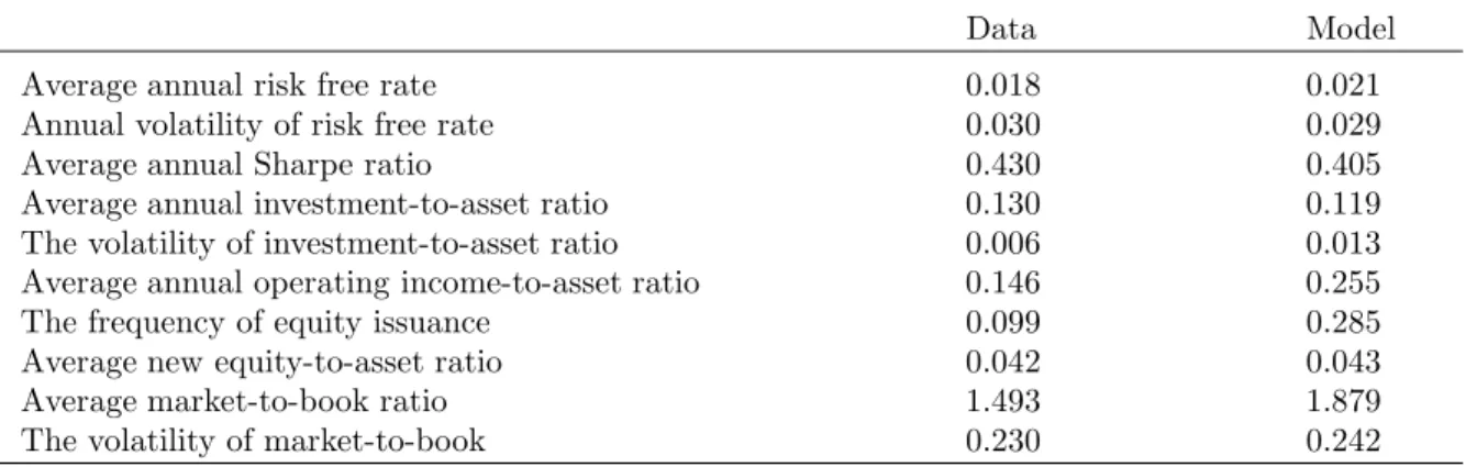
Table 1 reports our calibration of parameter values. Other than a few exceptions, these parameter values are similar to those used in Zhang (2005b). Using this parametrization, we solve the model using the standard value function iteration technique (see Appendix A for a detailed description of our algorithm). We then simulate the model using the value function and optimal policy functions to create an artificial panel of 5000 firms with 480 monthly observations for each firm. This procedure is repeated 100 times. Table 2 reports the model-implied unconditional sample moments averaged across these 100 simulations.
The overall fit reported in Table 2 seems reasonably good. The mean and volatility of risk-free rate and the average Sharpe ratio simulated from the model are very close to those observed in the data. This fit is perhaps not surprising because we pin down three
Table 1 : Parameter Choices
This table reports our parameter choices. We need to calibrate 14 parameters: the capital shareα; the long-run average level of aggregate productivity ¯x; the persistence of aggregate productivityρx; the conditional volatility of aggregate productivity shocksσx; the persistence of firm-specific productivityρz; the conditional volatility of firm-specific productivity shocksσz; the three parameters in the stochastic discount factor η,
γ0, andγ1; the fixed cost of productionf; the rate of capital depreciationδ; the adjustment-cost parameter
a; the fixed cost of financingλ0; and the proportional factor of financing costsλ1.
α x¯ ρx σx ρz σz η γ0 γ1 f δ a λ0 λ1
0.70 −3.751 0.951/3 0.007/3 0.965 0.100 0.994 50 −1000 0.005 0.01 15 0.08 0.025
parameters, η, γ0, and γ1, using exactly these three moments. The model moments of the
investment-to-asset ratio are also close to its data moments. The average market-to-book ratio in the model, 1.88, is close to that in the data, 1.49. One caveat is that the frequency of equity issuance in the model, 28.5%, is much higher than that in the data, 9.9%. The reason is probably that in the model external equity is the only source of outside funds.
Figure 1 plots our numerical solutions of the value function and the optimal investment policy against the endogenous state variable, capital stock k, and the two exogenous state variables, aggregate productivityx and firm-specific productivityz. Because there are three state variables, we first fix x= ¯x and plot the functions against k and z in Panels A and C. We then fixz= ¯z and plot the functions againstk and x in Panels B and D. From Panels A and B, because of decreasing return to scale, firm value is increasing and concave function of capital k. The value function also increases with aggregate productivity x and firm-specific productivityz. From Panels C and D, investment-to-asset decreases with capital stock kbut increases with aggregate and firm-specific productivity. Our model thus predicts that small firms with relatively less assets-in-place and growth firms with relatively high profitability tend to invest more and grow faster, consistent with Fama and French (1995).
Figure 1 : The Value Function and Optimal Investment Policy Function
This figure plots the value function v(k, z, x) and the investment-to-asset ratio i
k(k, z, x) as functions of one endogenous state variablek, and two exogenous state variablesx and z. Because there are three state variables, we fixx= ¯xand plot the value and policy functions againstkandzin Panels A and C, respectively, in which the arrows indicate the direction along whichzincreases. We then fixz= ¯zand plot the value and policy functions againstkandxin Panels B and D, respectively, in which the arrows indicate the direction along whichxincreases.
Panel A:v(k, z,x¯) Panel B:v(k,z, x¯ ) 0 2 4 6 8 10 0 5 10 15 20 25 k v z 0 2 4 6 8 10 0 2 4 6 8 10 12 14 16 k v x Panel C: i k(k, z,x¯) Panel D: i k(k,z, x¯ ) 0 2 4 6 8 10 −0.2 0 0.2 0.4 0.6 0.8 1 1.2 1.4 1.6 k i/k z 0 2 4 6 8 10 −0.2 0 0.2 0.4 0.6 0.8 1 1.2 k i/k x
Table 2 : Unconditional Moments from the Simulated and Real Data
This table reports unconditional sample moments generated from the simulated data and from the real data. We simulate 100 artificial panels each of which has 5000 firms and 480 monthly observation. We report the cross-simulation averaged results. The average Sharpe ratio in the data is from Campbell and Cochrane (1999). The data moments of the real interest rate are from Campbell, Lo, and MacKinlay (1997). All other data moments are from Hennessy and Whited (2005).
Data Model
Average annual risk free rate 0.018 0.021
Annual volatility of risk free rate 0.030 0.029
Average annual Sharpe ratio 0.430 0.405
Average annual investment-to-asset ratio 0.130 0.119
The volatility of investment-to-asset ratio 0.006 0.013
Average annual operating income-to-asset ratio 0.146 0.255
The frequency of equity issuance 0.099 0.285
Average new equity-to-asset ratio 0.042 0.043
Average market-to-book ratio 1.493 1.879
The volatility of market-to-book 0.230 0.242
Based on the optimal investment-to-asset ratio, we plot in Figure 2 the implied new equity-to-asset ratio and the payout-to-asset ratio from equations (8) and (10). From Panels A and B, the new equity-to-asset ratio closely mimics the patterns of the investment-to-asset ratio. Small firms with relatively less capital and growth firms with relatively high firm-specific productivity tend to issue more equity. This prediction is largely consistent with the evidence documented in Barclay, Smith, and Watts (1995) and Fama and French (2005). And from Panel B, firms tend to use more equity when aggregate economic conditions are relatively good, i.e., whenxis high, a pattern consistent with the evidence in Choe, Masulis, and Nanda (1993). Finally, from Panels C and D, the payout-to-asset ratio increases with capital stock, although the relation is not strictly monotonic. Small firms with less assets distribute relatively little cash, while big firms with more assets distribute more. This prediction also is consistent with Barclay et al., who report that dividend yields correlate positively with the log of total sales, a measure of firm size.
Figure 2 : Optimal Equity-Financing and Payout Police-Functions
This figure plots the new equity-to-asset ratio ke(k, z, x) and the payout-to-asset ratio dk(k, z, x) as functions of one endogenous state variable, capital stock k, and two exogenous state variables, aggregate and firm-specific productivityx andz. Because there are three state variables, we fix x= ¯x and plot the functions againstk andz in Panels A and C, in which the arrows indicate the direction along which z increases. In Panels B and D, we fixz= ¯z and plot the functions againstkandx, and the arrows indicate the direction along whichxincreases.
Panel A: e k(k, z,x¯) Panel B: e k(k,¯z, x) 0 2 4 6 8 10 0 2 4 6 8 10 12 14 16 18 k e/k z 0 2 4 6 8 10 0 2 4 6 8 10 12 k e/k x Panel C: dk(k, z,x¯) Panel D: dk(k,z, x¯ ) 0 2 4 6 8 10 0 0.005 0.01 0.015 0.02 0.025 0.03 k d/k z 0 2 4 6 8 10 0 0.005 0.01 0.015 0.02 0.025 0.03 0.035 k d/k x
4
Empirical Implications
We now investigate whether our model can quantitatively reproduce the relations between stock returns and financing decisions that have attracted considerable attention in recent em-pirical corporate finance literature. We follow the quantitative-theory approach of Kydland and Prescott (1982) and Berk, Green, and Naik (1999) to conduct computational experi-ments to compare the model moexperi-ments with those in the data. Specifically, we simulate 100 artificial panels, each of which has 5,000 firms and 480 months. And the sample size is com-parable to the COMPUSTAT data set often used in empirical studies. We then implement empirical procedures on each artificial panel, report cross-simulation averaged results, and compare them to their counterparts in the real data.
We aim at a broad range of empirical studies in the literature. We first study the cyclical properties of equity issuance as applied to equity issuance waves and the predictive rela-tions between the new equity share and aggregate stock market returns. Then we examine the long-run stock-price performance and operating performance of issuing firms, as well as the long-run stock-price performance of cash-distributing firms. Finally, we generate the negative investment-return relation which is at the heart of our economic mechanisms.
4.1
Equity Issuance Waves
A larger number of firms issue common stocks and the proportion of external financing ac-counted for by equity is substantially higher in economic expansions (e.g., Taggart (1977), Marsh (1982), and Choe, Masulis, and Nanda (1993)). In particular, Choe et al. docu-ment that the relative frequency of equity offers, defined as the number of equity offerings per month scaled by the number of listed firms, and the dollar volume of security offerings scaled by CPI are both procyclical. And in multiple regressions, the new equity share,
de-fined as the ratio of common stock issues to the sum of common stock and bond issues in dollar volume per month, increases with business cycle measures such as the growth rate of industrial production, and decreases with stock market volatility. Finally, neither stock market run-up nor interest rate changes have significant explanatory power in the presence of business cycle measures and stock market volatility.
We ask whether our model can reproduce these empirical patterns. As in Zhang (2005b), we define expansions in artificial data to be times when aggregate productivity is at least one unconditional standard deviation above its long-run average, i.e., xt>x¯+√σx
1−ρ2
x
. And we define contractions to be times when aggregate productivity is at least one unconditional standard deviation below its long-run average, i.e., xt<x¯−√σx
1−ρ2
x
. We measure the relative frequency of equity issuance in the model as
PN
j=11{ejt>0}
N , where
1{ejt>0} is the indicator function that takes a value of one if firm j issues equity and zero
otherwise. N is the total number of firms in the economy. Because we do not model entry and exit in the model, N remains constant over time. More important, incorporating entry and exit is likely to reinforce our basic results. The reason is that the frequency of entry or Initial Public Offerings tends to be procyclical and the frequency of exit or delisting tends to be countercyclical, as shown in Pastor and Veronesi (2005).
We define the rate of aggregate equity financing as the total amount of new equity divided by total assets:
PN j=1ejt
PN
j=1kjt. And because we do not model debt, we define the new equity share
as the share of new equity out of total amount of financing or the sum of new equity and internal funds:
PN j=1ejt
PN
j=1(ejt+yjt). We caution that our definition of the equity share does not
correspond exactly with the definition in the empirical literature (e.g., Baker and Wurgler (2000)). But our definition seems to capture the essence underlying the new equity share without complicating greatly the basic model structure.
Table 3 : Conditional Moments of Equity Issuance
This table reports conditional moments of equity issuance from simulated panels. We report the average frequency of equity issuance, the rate of aggregate equity financing, and the share of new equity in total financing, all conditional on the economy being in expansions or contractions. We define expansions in simulated panels to be times when aggregate productivity is at least one unconditional standard deviation above its long-run average, i.e., xt >x¯+√σx
1−ρ2 x
, and we define contractions to be times when aggregate productivity is at least one unconditional standard deviation below its long-run average, i.e.,xt<x¯−√σx
1−ρ2 x . The relative frequency of equity issuance is defined in the model as
PN
j=11{ejt >0}
N , where 1{ejt>0} is the
indicator function that takes a value of one if firmj issues equity and zero otherwise, andN= 5,000 is the total number of firms in the simulated economy. The rate of aggregate equity financing is defined as the total amount of new equity divided by total assets, i.e.,
PN
j=1ejt
PN
j=1kjt. Because we do not model debt, we measure the new equity share as the share of new equity out of total financing including both new equity and internal funds, i.e.,
PN
j=1ejt
PN
j=1(ejt+yjt)
. For simulations create 100 artificial panels each with 5000 firms and 480 monthly observations. The table reports the cross-simulation averaged results.
Panel A: Expansions Panel B: Contractions
The frequency The aggregate equity The new The frequency The aggregate equity The new of equity issuance financing rate equity share of equity issuance financing rate equity share
0.825 0.030 0.526 0.015 0.002 0.036
Using simulated panels, we compute the average frequency of equity issuance, the average rate of aggregate equity financing, and the average new equity share conditional on the economy being in expansions or contractions. Table 3 reports the results. We observe that equity issuance is strongly procyclical. The relative frequency of equity issuance is 82.5% in expansions, and is only 1.5% in contractions. The rate of aggregate equity financing is 3.0% in expansions and is 0.2% in contractions. Finally, the new equity share is 52.6% in expansions and is only 3.6% in contractions. This procyclical pattern in our simulations is consistent with the evidence in Choe, Masulis, and Nanda (1993).
We also use simulated data to regress contemporaneously the rate of aggregate equity financing and the new equity share onto the growth rate of aggregate output, defined as
PN j=1yjt
PN
j=1yjt−1, prior six-month stock market returns, defined as
PN j=1vjt
PN
Table 4 : Contemporaneous Regressions of the Rate of Aggregate Equity Financing and the New Equity Share in Total Financing onto Macroeconomic Variables
This table uses simulated data to regress contemporaneously the rate of aggregate equity financing,
PN
j=1ejt
PN
j=1kjt
and the share of new equity in total financing,
PN
j=1ejt
PN
j=1(ejt+yjt)
, onto the growth rate of aggregate output
PN
j=1yjt
PN
j=1yjt−1, prior six-month stock market returns
PN
j=1vjt
PN
j=1(vjt−5−djte −5), and stock market volatility estimated using the rolling prior 36 months of simulated data. We simulate 100 artificial panels, each has 5000 firms and 480 monthly observations. We perform the regressions on each simulated panel and report the cross-simulation average results. The numbers in parentheses are the cross-cross-simulation averagedt-statistics adjusted for heteroscedasticity and autocorrelations of up to 12 lags.
Panel A: The rate of aggregate equity financing Panel B: The new equity share
The growth rate of Prior six-month Stock market The growth rate of Prior six-month Stock market aggregate output market return volatility aggregate output market return volatility
1.62 23.20 (29.99) (37.49) 0.06 0.69 (14.04) (13.05) 0.32 2.92 (9.76) (6.90) 1.37 0.01 0.16 22.27 0.03 0.74 (22.68) (2.95) (7.69) (29.37) (0.77) (3.17)
market volatility estimated with the rolling prior 36 months of simulated data. From Table 4, the results are largely consistent with Choe, Masulis, and Nanda (1993). In particular, the rate of aggregate equity financing and the new equity share both correlate positively with the growth rate of industrial production and with the stock market returns.
4.2
Predicting Stock Market Returns with the New Equity Share
In an important article, Baker and Wurgler (2000) show that the share of new equity issues in total new equity and debt issues is a strong, negative predictor of future stock market returns. Baker and Wurgler interpret this evidence as suggesting that firms time the market compo-nent of their returns when issuing equity to exploit systematic mispricing in market returns. We show that our model without mispricing can largely replicate the Baker and Wurgler
Table 5 : Univariate, Predictive Regressions of One-Year-Ahead Market Returns
This table reports univariate, predictive regressions of annual percentage stock market returns on three regressors. The regression equation is rt+1=a+bXt+et+1, where rt denotes the real percentage returns on the value-weighted (vw) market portfolio or the equally-weighted (ew) market portfolio. Xt denotes the regressors including the dividend-to-price ratio, the book-to-market ratio, or the new equity share in the sum of total new equity and internal funds. The dividend-to-price ratio, the book-to-market ratio, and the equity share in new issues are standardized to have zero mean and unit variance. We simulate 100 artificial panels, each of which has 5000 firms and 480 monthly observations. We perform the predictive regressions on each simulated panel and report the cross-simulation averaged slopes and test statistics. For comparison, we also report in data columns the results from Table 3 of Baker and Wurgler (2000).
Panel A: Dividend-to-price Panel B: Book-to-market Panel C: The new equity share
Data Model Data Model Data Model
b t(b) b t(b) b t(b) b t(b) b t(b) b t(b)
vw 5.01 (2.12) 12.99 (3.38) 4.61 (1.79) 14.32 (3.81) −7.42 (−3.86) −10.49 (−2.59) ew 5.75 (2.04) 13.38 (3.50) 13.06 (2.83) 14.37 (3.84) −13.12 (−3.64) −10.47 (−2.60)
(2000) evidence. Specifically, we perform univariate, predictive regressions of one-year-ahead stock market returns on the dividend yield, defined in the model as
PN j=1djt
PN
j=1(vjt−dejt), on the
aggregate book-to-market, defined as PN
j=1kjt
PN
j=1(vjt−dejt), and on the new equity share. Following
Baker and Wurgler (2000), we standardize all the predictors so that they have zero mean and unit variance. The rationale is to make the slope coefficients of different regressors comparable to each other. And as dependent variables, we use annual percentage returns on both value-weighted and equal-weighted market portfolios.
Table 5 reports the results. The model largely reproduces the predictive regression results obtained in the data. The dividend yield and the aggregate book-to-market ratio are both significantly positive predictors of future stock market returns. More important, the new equity share is a significantly negative predictor of future stock market returns.
We caution again that our definition of the equity share in the model does not correspond exactly with that in Baker and Wurgler (2000). This difference makes direct comparison
be-tween our simulation results and their evidence somewhat difficult. However, our definition does capture the basic intuition underlying the predictive power of the new equity share, i.e., the strong procyclicality of the new equity share gives rise to its negative correlation with the countercyclical aggregate expected returns.
4.3
The
Long-Term
Underperformance
Following
Seasoned
Equity Offerings
In an influential contribution, Loughran and Ritter (1995) document that firms issuing eq-uity earn much lower returns on average over the next three to five years than nonissuing firms with similar characteristics (see also Spiess and Affleck-Graves (1995)). The magnitude of this underperformance varies over time. Firms issuing during light issuance periods do not underperform much, while firms issuing during high-volume periods severely underperform. To study whether our model can quantitatively generate this evidence, we replicate Loughran and Ritter’s (1995) analysis reported in their Table VIII. Specifically, we use simulated panels to perform Fama-MacBeth (1973) monthly cross-sectional regressions of percentage stock returns onto the market value, book-to-market, and an issue dummy:
rjt+1 =b0+b1 log(MEjt) +b2 log(BMjt) +b3ISSUEjt+jt+1 (18)
where rjt+1 is the percentage return on stock j in from the beginning of month t to the
beginning of month t+1, and all the regressors are dated at the beginning of month t. We define market value in the model to be the ex-dividend firm value, vjt−dejt, and book-to-market to be kjt
vjt−dejt. Following Loughran and Ritter (1995), we evaluate MEjt as the
market value of equity of firmj on the most recent fiscal year that ended prior to the month
ended prior to the montht. And ISSUEjt is a dummy variable that takes a value of one if firm
j has conducted one or more equity issues within the previous five years, and zero otherwise, i.e., ISSUEjt≡1{P59
τ=0ejt−τ>0}. We also halve the sample into months following light issuance
activity and months following heavy issuance activity. Specifically, we partition the sample on the basis of the fraction of the sample firms in a month that have issued equity during the prior five years. The light-issuance sample has all the months with the fraction below its median, and the heavy-issuance sample has all the months with the fraction above its median. From Table 6, the model does a decent job in reproducing the empirical evidence. When the issue dummy is used alone, issuing firms underperform by 0.49% per month in the data with a t-statistic of −3.98. And its model counterpart is 0.99% per month with a
t-statistic of −3.87. Controlling for size and book-to-market in the regressions reduces the underperformance to 0.38% in the data and to 0.64% in the model, and both are significant. More important, the model also reproduces quantitatively the positive relation between the magnitude of the underperformance and the volume of equity issuance. In the last two regressions in Table 6, we divide the sample periods into months following light issuance activity and months following heavy issuance activity. Loughran and Ritter (1995) show that issuing firms underperform by an insignificant amount of only 0.17% per month following light issuance activity but by a significant amount of 0.60% following heavy issuance activity. From the last column, issuing firms following light issuance activity in the model underperform by an insignificant 0.32% per month, while issuing firms following heavy issuance activity underperform by a significant 0.95% per month.
Table 6 : Fama-MacBeth (1973) Monthly Cross-sectional Regressions of Percentage Stock Returns on Size, Book-to-Market, and a New Issues Dummy
This table reports the Fama-MacBeth (1973) monthly cross-sectional regressions:rjt+1=b0+b1log(MEjt)+
b2 log(BMjt)+b3ISSUEjt+jt+1, whererjt+1denotes the percentage return on firmj during montht. MEjt
is the market value of firmj on the most recent fiscal year ending before montht. BMjt is the ratio of the book value of equity to the market value of equity for firmj on the most recent fiscal year ending before month t. And ISSUEjt is a dummy variable that equals one if firm j has conducted at least once equity offerings within the past 60 months preceding montht, and equals zero otherwise. The light-issuance sample has all the months with the fraction of issuing firms below its median, and the heavy-issuance sample has all the months with the fraction of issuing firms above its median. We simulate 100 artificial panels, each of which has 5000 firms and 480 monthly observations. We then perform the cross-sectional regressions on each simulated panel and report the cross-simulation averaged slopes and Fama-MacBetht-statistics. We also compare our results to those reported in Loughran and Ritter (1995, Table VIII).
Sample log(ME) log(BM) ISSUE
Data Model Data Model Data Model
All months − − − − −0.49 −0.99 − − − − (−3.98) (−3.87) All months −0.05 0.67 0.30 0.66 −0.38 −0.64 (−0.91) (4.52) (4.57) (8.36) (−3.68) (−2.87) Periods following −0.26 0.31 0.20 0.42 −0.17 −0.32 light volume (−3.12) (2.28) (1.80) (5.77) (−1.19) (−0.90) Periods following 0.16 1.03 0.39 0.90 −0.60 −0.95 heavy volume (2.11) (6.16) (6.30) (9.43) (−3.98) (−4.24)
4.4
The Long-Term Operating Performance Following Seasoned
Equity Offerings
In another influential article, Loughran and Ritter (1997) document that the operating performance of issuing firms displays substantial improvement prior to the equity offerings, but then deteriorates. Issuing firms are also disproportionately investing and high-growth firms. The authors interpret their evidence as consistent with Jensen’s (1993) hypothesis that corporate culture excessively focuses on growth, and managers are as overoptimistic about the future profitability of the issuing firms as outside investors.
reproduce the Loughran and Ritter (1997) evidence. To this end, we use simulated panels to replicate their Table II by reporting the medians of the operating performance for issuing firms and matching firms for nine years around the issuance. Specifically, following Loughran and Ritter, we choose matching nonissuers by matching each issuing firm with a firm that has not issued equity during the prior five years as follows. If there is at least one nonissuer in the same industry with end-of-year zero assets within 25 to 200 percent of the issuing firm, the nonissuer with the closest operating income-to-asset ratio is used.2 We also report
theZ-statistics testing the equality of distributions between the issuers and nonissuers using the Wilcoxon matched-pairs signed-ranks test, and the Z-statistics testing the equality of distributions between the changes in the ratios from year 0 to year +4.3 Under the null
hypothesis that the issuer and the nonissuer measures are drawn from the same distribution,
Z follows a standard normal distribution.
We consider four operating performance measures: (i) OIBD/assets, where OIBD denotes operating income before depreciation, measured as yjt
kjt in the model; (ii) return on assets
or profitability, measured as kjt+1−kjt+dejt
kjt in the model, (iii) the investment-to-asset ratio,
measured as ijt
kjt in the model; and (iv) market-to-book, measured as
vjt−dejt
kjt in the model.
Table 7 reports the quantitative results. Consistent with the evidence in Loughran and Ritter (1997), issuers in the model experience deterioration in the operating performance. After equity issuance, the operating income-to-asset ratios and profitability of issuers become significantly lower than those of nonissuers. However, the model-implied operating
income-2In the real data, if no nonissuer meets this criterion, Loughran and Ritter (1997) then rank all nonissuers
with year 0 assets of 90 to 110 percent of the issuer, and the firm with the closest, but higher operating income-to-asset ratio is used. Because we do not distinguish different industries in the model, we simply use the 25 to 200 percent restriction on end-of-year zero assets to choose matching nonissuer.
3Denote the difference in the accounting measure between issuer i and its matching firm by diff
i ≡ measure(issueri)−measure(nonissueri). We rank the absolute values of the diffi from 1 to Ne, the total number of issuing firms. We then sum the ranks of positive values of diffi, and denote the sum withD. The
Z-statistics are computed asZ=D−σDE[D], where E[D] =Ne(N4e+1) andσD=N
e(Ne+1)(2Ne+1)
to-asset and profitability levels are on average much higher than those observed in the data. The reason is probably that the denominator in the model variables corresponds to the fixed assets in the data, which are only part of the total assets.
What drives the deteriorating accounting performance of firms after issuing equity? Intu-itively, the firm-level profitability in the model is driven by the persistent and mean-reverting firm-specific productivity in equation (2). Therefore, ex-post, issuers tend to be firms that have recently experienced extremely high firm-specific shocks, εz
jt+1. But going forwards,
is-suers face the same conditional, standard normal distribution of these shocks as other firms do. When we as econometricians look at the historical sample, we are likely to observe the mean-reverting behavior in the cross-sectional difference in productivity, zjt, measured empirically as the differences in profitability between issuers and matching nonissuers.
Table 7 also shows that issuers in the model have persistently higher investment-to-asset and market-to-book ratios than matching nonissuers. And from Panel C, these differences are mostly significant. Moreover, the model does a decent job in matching the mean-reverting behavior of the investment-to-asset and market-to-book ratios.
4.5
The Long-Term Performance of Firms Distributing Cash
When firms raise capital, they underperform matching firms in the future three to five years. But when firms distribute cash back to shareholders, they outperform matching firms. For example, Ikenberry, Lakonishok, and Vermaelen (1995) show that the average abnormal four-year buy-and-hold return after the announcements of open market share repurchases is 12.1% in 1980–1990. And the average abnormal return is 45.3% for value firms, but is insignificantly negative for growth firms. Similarly, Michaely, Thaler, and Womack (1995) show that stock prices continue to drift in the same direction in the years following the
Table 7 : Median Operating Performance Measures and Market-to-Book for Issuers and Matching Nonissuers
Panels A and B report the median operating performance measures for the issuing and matching firms. Panels C and D report theZ-statistics testing the equality of distributions between the issuers and matching nonissuers using the Wilcoxon matched-pairs singed-ranks test. We simulate 100 artificial panels, each of which has 5000 firms and 480 monthly observations. The monthly flow variables are aggregated within a given year to create annual variables. Stock variables are measured at the beginning of the year. We perform the tests on each simulated panel and report the cross-simulation average results. We also compare our results to those reported in Table II of Loughran and Ritter (1997).
Event year Operating Profitability Investment- Market-to-book
income-to-asset to-asset
Panel A: Issuer medians
Data Model Data Model Data Model Data Model
−4 16.1% 26.0% 5.8% 12.7% 8.2% 0.6% 1.20 1.45 −3 16.6% 26.9% 6.0% 16.0% 8.5% 1.8% 1.42 1.54 −2 16.4% 28.5% 6.0% 19.6% 9.9% 7.0% 1.59 1.77 −1 17.0% 30.1% 6.4% 23.4% 10.2% 13.5% 2.40 1.95 0 15.8% 27.8% 6.3% 27.2% 10.0% 23.1% 1.96 2.48 +1 14.2% 25.8% 5.3% 15.7% 10.6% 23.4% 1.68 2.22 +2 12.7% 24.5% 3.9% 13.1% 9.3% 19.2% 1.65 2.09 +3 12.1% 23.6% 3.3% 13.3% 8.7% 16.6% 1.58 2.00 +4 12.1% 23.0% 3.2% 13.1% 8.1% 14.7% 1.43 1.97
Panel B: Nonissuer medians
Data Model Data Model Data Model Data Model
−4 16.4% 25.5% 6.1% 9.9% 5.0% 3.5% 1.04 1.48 −3 15.6% 25.8% 5.8% 12.2% 5.4% 1.3% 1.12 1.45 −2 15.4% 26.3% 5.3% 14.0% 5.6% 0.6% 1.19 1.45 −1 15.1% 27.0% 5.5% 15.7% 5.7% 1.2% 1.30 1.48 0 15.8% 27.8% 5.7% 17.4% 5.9% 3.0% 1.45 1.55 +1 15.2% 26.8% 5.3% 19.7% 6.5% 6.4% 1.41 1.69 +2 14.1% 25.6% 4.8% 18.3% 6.5% 10.1% 1.43 1.81 +3 13.8% 24.8% 4.6% 16.3% 6.6% 12.0% 1.48 1.86 +4 13.5% 24.2% 4.2% 15.8% 6.6% 13.4% 1.44 1.91
Panel C:Z-statistics testing the equality of distributions between the issuers and matching nonissuers
−4 −0.92 −0.03 −2.10 4.84 12.00 −8.26 3.65 −4.14 −3 2.87 −2.74 1.12 9.36 13.69 3.71 5.64 10.41 −2 4.73 −7.48 3.42 15.40 16.16 23.56 8.87 32.07 −1 7.68 −14.69 6.58 23.56 17.10 43.96 16.98 42.53 0 −1.06 −49.80 6.50 32.77 15.46 49.58 10.36 47.56 +1 −3.02 5.65 0.35 −13.83 14.55 40.27 7.52 26.60 +2 −5.29 4.92 −5.26 −16.29 11.24 20.57 4.11 11.81 +3 −5.40 4.90 −6.58 −8.70 8.64 8.81 1.74 1.44 +4 −4.43 4.64 −5.76 −7.54 7.91 0.63 −0.51 −0.85 Panel D:Z-statistics testing the equality of distributions
announcements of dividend initiations and omissions.
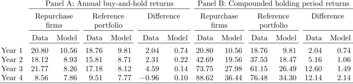
To study whether our model can quantitatively generate these empirical results, we replicate Tables 3 and 4 in Ikenberry, Lakonishok, and Vermaelen (1995) using our simulated panels. In the model, we identify firms with positive dividends as those conducting stock repurchase in the data. Our model only pins down the total amount of payout, not its specific forms: the Miller-Modigliani (1991) dividend irrelevancy theorem holds in our neoclassical model. We report mean annual returns from buying an equally-weighted portfolio of repurchasing firms, beginning in the month following the repurchase and for the subsequent four years. We also report total compounded returns for up to four years, and compare the returns of the cash-distributing firms to returns of reference portfolio.
We follow closely Ikenberry, Lakonishok, and Vermaelen (1995) in forming our reference portfolio. All firms in our simulated panel are sorted each month into one of 50 size and market portfolios by taking the intersections of ten size deciles and five book-to-market quintiles. Then all firms are ranked in the beginning of calendar year and are held for the following 12 months. Beginning in the next month, the one-year buy-and-hold return is calculated for each firm in a given portfolio. We use the equally-weighted average of all annual returns in a given portfolio as the benchmark return for the firms ranked in that particular size and book-to-market portfolio. The ranking of a particular firm may change from year to year. To accommodate this feature, we allow the benchmark to change over time. Table 8 reports annual buy-and-hold returns and compounded holding period returns up to four years following share repurchases, both in the data and in the model. The table shows that cash-distributing firms indeed earn higher average returns than nondistributing firms. But the magnitudes of the differences seem much lower in the simulated data than those in the real data.
Table 8 : Annual Buy-and-Hold Returns and Compounded Holding Period Returns Up to Four Years Following Market Share Repurchases
This table reports annual and compounded buy-and-hold percentage returns following share repurchases for up to four years. Compounded holding-period returns assume annual rebalancing. We form equally-weighted portfolios for the whole sample. We construct the reference portfolio using benchmark returns corresponding to the repurchase sample, matched on the basis of size and book-to-market ranking. To form reference portfolio, we sort all firms in our simulated panel each month into one of 50 size and book-to-market portfolios (the intersections of ten size deciles and five book-to-book-to-market quintiles). We rank all firms in the beginning of calendar year and hold them for the following 12 months. Beginning in the next month, we calculate the one-year buy-and-hold return for each firm in a given portfolio. We then use the equal-weighted average of all annual returns in a given portfolio as the benchmark returns for firms ranked in that particular size and book-to-market portfolio. We rebalance the portfolio annually. We simulate 100 artificial panels, each of which has 5000 firms and 480 monthly observations. We perform the empirical analysis on each simulated panel and report the cross-simulation average results. We also compare our results to those reported in Table 3 of Ikenberry, Lakonishok, and Vermaelen (1995).
Panel A: Annual buy-and-hold returns Panel B: Compounded holding period returns Repurchase Reference Difference Repurchase Reference Difference
firms portfolio firms portfolio
Data Model Data Model Data Model Data Model Data Model Data Model Year 1 20.80 10.56 18.76 9.81 2.04 0.74 20.80 10.56 18.76 9.81 2.04 0.74 Year 2 18.12 8.93 15.81 8.71 2.31 0.22 42.69 19.56 37.53 18.47 5.16 1.06 Year 3 21.77 8.26 17.18 8.12 4.59 0.14 73.75 27.98 61.15 26.49 12.60 1.49 Year 4 8.56 7.86 9.51 7.77 −0.96 0.10 88.62 36.44 76.48 34.30 12.14 2.14
We also examine the annual buy-and-hold returns and compounded holding-period returns following cash distribution by book-to-market quintiles. We rank all firms into size deciles, and further sort each decile into market quintiles. The lowest book-to-market ratios are assigned to quintile one. We form the reference portfolio using benchmark returns corresponding to the repurchase sample, matched on size and book-to-market.
From Table 9, the model can reproduce the empirical pattern that the magnitude of the long-run stock-price drift following cash distribution is stronger in value firms than that in growth firms (e.g., Ikenberry, Lakonishok, and Vermaelen (1995, Table 4)). However, the magnitudes of the drift in the model are again much lower than that observed in the data.
Table 9 : Annual Buy-and-Hold Returns and Compounded Holding Period Returns by Book-to-Market Quintiles Following Cash Distribution
This table reports annual and compounded buy-and-hold percentage returns for equally-weighted portfolios of firms distributing cash for up to four years following market share repurchases by book-to-market quintile ranking. Compounded holding-period returns assume annual rebalancing. Ranks are determined by sorting all firms into size deciles. Each decile is further sorted into quintiles on the basis of book-to-market, with the lowest ratios assigned to quintile one. We form the reference portfolio using benchmark returns corresponding to the repurchase sample, matched on the basis of size and book-to-market ranking. We create 100 artificial panels of 5000 firms each and with 480 observations for each firm. The unit time period is one month. We perform these analysis on each simulated panel and report across-simulation averaged results, and we compare our results to those reported in Ikenberry, Lakonishok, and Vermaelen (1995, Table 4).
Annual buy-and-hold returns Compounded holding period returns Repurchase Reference Difference Repurchase Reference Difference
firms portfolio firms portfolio
Data Model Data Model Data Model Data Model Data Model Data Model Panel A: Book-to-market quintile 1 (growth stocks)
Year 1 15.72 11.17 16.83 10.47 −1.11 0.70 15.72 11.17 16.83 10.47 −1.11 0.70 Year 2 17.86 9.95 16.60 9.83 1.26 0.12 36.40 21.46 36.22 20.56 0.18 0.90 Year 3 12.00 9.46 13.61 9.38 −1.61 0.07 52.77 31.73 52.77 30.51 −1.98 1.23 Year 4 4.98 9.14 6.42 9.04 −1.44 1.11 60.38 42.42 60.38 40.55 −4.31 1.89
Panel B: Book-to-market quintile 2
Year 1 20.59 10.98 18.43 10.33 2.16 0.65 20.59 10.98 18.43 10.33 2.16 0.65 Year 2 12.34 9.51 15.07 9.36 −2.73 0.14 35.47 20.67 36.28 19.79 −0.81 0.88 Year 3 22.39 8.85 17.29 8.77 5.10 0.08 65.80 29.99 59.84 28.74 5.96 1.25 Year 4 3.20 8.51 6.99 8.41 −3.79 0.10 71.10 39.47 71.02 37.54 0.08 1.93
Panel C: Book-to-market quintile 3
Year 1 19.49 10.90 16.46 10.29 3.03 0.62 19.49 10.90 16.46 10.29 3.03 0.62 Year 2 18.23 9.31 17.33 9.11 0.90 0.20 41.27 20.28 36.64 19.38 4.63 0.91 Year 3 20.77 8.48 16.57 8.36 4.20 0.12 70.61 28.98 59.29 27.67 11.32 1.32 Year 4 7.45 8.09 10.35 8.01 −2.90 0.09 83.32 37.71 75.78 35.71 7.54 2.00
Panel D: Book-to-market quintile 4
Year 1 23.43 10.81 22.84 10.19 0.59 0.62 23.43 10.81 22.84 10.19 0.59 0.62 Year 2 15.16 8.98 12.73 8.78 2.43 0.20 42.14 19.78 38.48 18.84 3.66 0.93 Year 3 24.05 8.04 18.32 7.90 5.73 0.14 76.32 27.84 63.85 26.44 12.47 1.40 Year 4 12.44 7.65 11.06 7.53 1.38 0.12 98.24 35.82 81.97 33.69 16.27 2.13
Panel E: Book-to-market quintile 5 (value stocks)
Year 1 24.15 10.50 19.49 9.69 4.66 0.82 24.15 10.50 19.49 9.68 4.66 0.82 Year 2 26.01 8.35 17.23 8.08 8.78 0.27 56.44 18.72 40.08 17.51 6.36 1.21 Year 3 29.81 7.38 20.49 7.21 9.32 0.17 103.07 25.94 68.78 24.23 34.29 1.71 Year 4 16.17 6.87 12.94 6.77 3.23 0.10 135.91 32.86 90.62 30.50 45.29 2.37
4.6
Capital Investment, External Finance, and Stock Returns
The finance-related anomalies are intimately linked to the investment-return relation. Richardson and Sloan (2003) document that the negative relation between external finance and future stock returns varies systematically with the use of the proceeds. When the pro-ceeds are invested in net operating assets as opposed to being stored as cash, there exists a stronger negative relation. And there is no evidence on the negative relation for refinancing transactions. Lyandres, Sun, and Zhang (2005) document that adding a return factor based on real investment into calendar-time factor regressions makes underperformance following equity issuances largely insignificant and reduces its magnitude by 37–46%. This evidence highlights the importance of capital investment in driving the financing-related anomalies.
To study the investment-return relation in our model, we reproduce the main empirical analysis of Titman, Wei, and Xie (2004), who recently document a negative, firm-level relation between capital investment and average subsequent returns.4 Both Richardson and
Sloan and Titman et al. interpret this evidence as investors underreaction to empire building implications of real investment. As we show below, our model without underreaction or empire building can quantitatively reproduce the negative investment-return relation.
To this end, we use simulated panels to form five portfolios based on capital investment (abbreviated as CI hereafter). Following Titman, Wei, and Xie (2004), we define CI that corresponds to the portfolio formation year t as CIjt−1=(CE CEjt−1
jt−2+CEjt−3+CEjt−4)/3 −1, where CEjt−1 is firm j’s capital expenditure scaled by sales during year t−1. We measure CEjt−1
in the model as the investment-to-output ratio, ijt−1
yjt−1, because the output price is normalized to be one. The last three-year moving-average capital expenditure in the denominator of
4This negative investment-return relation is well-known in the aggregate data, see Cochrane (1991). Other
empirical studies documenting the negative investment-return relation in the firm-level include Anderson and Garcia-Feij´oo (2005), Lyandres, Sun, and Zhang (2005), and Xing (2005).
CIjt−1 is used to project the firm’s benchmark investment.
In the beginning of year t, we sort all firms into quintiles based on their year t−1 CI measures in ascending order. The firms remain in these portfolios for the whole year t; the portfolios are rebalanced annually. We then construct a CI-spread portfolio that has a long position in the two lowest CI portfolios and a short position in the two highest CI portfolios. The returns for this zero-cost portfolio are calculated by subtracting the average returns of the highest CI portfolios from the average returns of the lowest CI portfolios.
We also calculate the value-weighted monthly excess returns for each CI portfolio from year t tot+ 1. Following Titman, Wei, and Xie (2004), we measure excess returns relative to benchmarks constructed to have similar firm characteristics such as size, book-to-market, and price momentum. Specifically, we form 125 benchmark portfolios that capture these characteristics. Starting in yeart, the universe of common stocks is sorted into five portfolios based on firm size at the end of year t−1. And the breakpoints for size are obtained by sorting all firms into quintiles based on their size measures at the end of yeart−1 in ascending order. The size of each firm in our sample is then compared with the breakpoints to decide which portfolio the firm belongs to. Firms in each size portfolio are further equally sorted into quintiles based on their book-to-market ratio at the end of yeart−1. Finally, the firms in each of the 25 size and book-to-market portfolios are equally sorted into quintiles based on their prior-year return. In all, we obtain 125 benchmark portfolios.
We calculate excess returns using these 125 characteristic-based benchmark portfolios. Each year, each stock is assigned to a benchmark portfolio according to its rank based on size, book-to-market, and prior returns. Excess monthly returns of a stock are then calculated by subtracting the returns of the corresponding benchmark portfolio from the returns of this particular stock. The excess returns on individual stocks are then used to calculate the
value-weighted excess monthly returns on the test portfolios that are formed based on CI. Table 10 reports the results both in the data and in the simulations. Consistent with Titman, Wei, and Xie (2004), Panel A reports that firms with low CI earn higher average returns than firms with high CI. The model-implied average CI-spread is 10.6% per annum, which falls short of that documented in the data, 16.9%.
We also perform the following Fama-MacBeth cross-sectional regressions
rjt+1 =λ0t+λ1tCIjt+λ2tCIjt×DCFjt+jt+1 (19)
where rjt+1 is the benchmark-adjusted value-weighted return on individual stock i during
periodt. DCF is the dummy variable based on the cash flow, measured as operating income scaled by total assets, yjt
kjt in the model. If firm j’s cash flow is above the median cash flow
of the year, DCF equals one, otherwise it equals zero.
Panel B of Table 10 suggests that, consistent with Titman, Wei, and Xie (2004), there exists a negative correlation between future stock return and capital investment in the sim-ulated data. And the magnitude of this correlation increases with the operating income-to-asset ratio, as shown by the negative slope of λ2t for the interaction term, CIjt×DCFjt. The model-implied slopes are also quantitatively similar to those observed in the data.
5
Related Literature
We briefly discuss our connection to the literature in this section. Brav, Geczy, and Gompers (2000) document that the underperformance following seasoned equity offerings is concentrated primarily in small-growth issuing firms, and suggest that the underperformance reflects a more pervasive return pattern related to size and book-to-market. We provide an
Table 10 : Excess Returns of Capital Investment (CI) Portfolios
Panel A presents the distribution of excess returns on five CI portfolios and the CI-spread portfolio. CI denotes the capital investment measure. We use investment-to-asset ratio to create the CI portfolios. We report the monthly mean excess returns, the standard deviation, the maximum, the median, and the minimum of the excess returns. The CI portfolios are constructed as follows. In year t, all stocks are sorted into quintiles based on their CI measures in ascending order to form five CI portfolios. Value-weighted monthly excess returns on a portfolio are calculated from yeart to yeart+1. The excess return on an individual stock at time t is calculated by subtracting the returns of characteristic-based benchmark portfolios from the stock return at timet. The CI-spread denotes the zero-investment portfolio that has a long position in the two lowest CI portfolios and a short position in the two highest CI portfolios. The return series for this portfolio is calculated by subtracting the sum of the returns on the highest two portfolios from that on the two lowest CI portfolios, and then dividing the result by two. All portfolios are rebalanced annually. Panel B reports the results of the Fama-MacBeth (1973) cross-sectional regression:
rjt+1=λ0t+λ1tCIjt+λ2tCIjtDCFjt+jt+1, whererjt+1is the benchmark-adjusted value-weighted return on
individual stockj at during montht. DCF is the dummy variable based on cash flow, measured as operating income scaled by total assets, measured in the model as yjtkjt. If the cash flow of one firm is above the median cash flow of the year, its DCF equals one, and zero otherwise. We simulate 100 artificial panels, each of which has 5000 firms and 480 monthly observations. The monthly flow variables are aggregated within one given year to create their corresponding annual variables. We perform the tests on each simulated panel and report the cross-simulation average slopes and test statistics. We also compare our results to those reported in Table 1 (Panel A) and Table 6 (Panel A) in Titman, Wei, and Xie (2004).
Panel A: Excess return distribution of capital investment portfolios
CI Portfolio Mean Std Max Median Min
Data Model Data Model Data Model Data Model Data Model
Lowest 0.042 0.066 0.010 0.048 3.38 0.16 0.06 0.07 −3.11 −0.06 2 0.083 0.011 0.007 0.031 2.26 0.08 0.10 0.01 −2.76 −0.06 3 0.055 −0.006 0.006 0.023 1.84 0.05 0.03 −0.01 −2.07 −0.06 4 −0.083 −0.021 0.005 0.027 1.38 0.04 −0.06 −0.02 −1.88 −0.08 5 −0.127 −0.040 0.010 0.045 2.61 0.06 −0.08 −0.04 −4.08 −0.14 CI-spread 0.169 0.106 0.009 0.003 3.30 0.071 0.12 0.07 −2.63 0.05
Panel B:rjt+1=λ0t+λ1tCIjt+λ2tCIjt×DCFjt+jt+1
CI CI×DCF
Data Model Data Model
λ −0.79 −0.64 −0.76 −0.45
economic explanation of their evidence because the model suggests that both equity issuers and small-growth firms are high-investing firms.
Eckbo, Masulis, and Norli (2000) report that a multifactor asset pricing model can reduce the underperformance to an insignificant level, and argue that issuing firms are less risky because their leverage ratios are lowered as a result of equity issuance. We complement their work by suggesting the investment-based mechanism that can potentially drive their risk evidence. Moreover, Lyandres, Sun, and Zhang (2005) document that even after equity issuance, issuing firms have book and market leverage ratios substantially higher than those of matching nonissuers, inconsistent with the leverage explanation of the underperformance. Schultz (2003) argues that using event studies is likely to find long-term underperformance ex post, even though there is no underperformance ex ante.5 Weighing each period equally as
in calendar-time factor regressions solves this problem. We add to Schultz’s (2003) pseudo-market-timing insight in two ways. First, we provide an economic explanation for his key premise that firms are more likely to issue when stock prices are high so they can receive more for their equity. We show that optimal equity financing is highly procyclical, i.e., firms invest more and thus naturally issue more equity in expansions when stock prices are relatively high. Second, our argument applies to event-time as well as calendar-time evidence because the model predicts that issuing firms are expected to earn lower rates of returns ex ante.
Our work is also related to several other papers casting some doubt on behavioral mar-ket timing, but from the perspective of capital structure choice. Leary and Roberts (2005) argue that the persistence of leverage is likely driven by dynamic optimizing behavior with adjustment costs. Hennessy and Whited (2005) construct a dynamic trade-off model with
5If early in a sample period, issuing firms underperform, there will be few issues in the future because
investors are less interested in them. The average performance will be weighed more towards the early issues that underperformed. If early issuing firms outperform, there will be many more issues in the future. The early performance will be weighed less in the average performance.