Working PaPer SerieS
no 944 / oCToBer 2008
The neW area-Wide
Model of The
euro area
a MiCro-founded
oPen-eConoMy Model
for foreCaSTing and
PoliCy analySiS
W O R K I N G PA P E R S E R I E S
N O 9 4 4 / O C T O B E R 2 0 0 8
In 2008 all ECB publications feature a motif taken from the 10 banknote.
THE NEW AREA-WIDE MODEL
OF THE EURO AREA
A MICRO-FOUNDED OPEN-ECONOMY
MODEL FOR FORECASTING
AND POLICY ANALYSIS
1by Kai Christoffel, Günter Coenen
and Anders Warne
2This paper can be downloaded without charge from http://www.ecb.europa.eu or from the Social Science Research Network electronic library at http://ssrn.com/abstract_id=1271865.
1 We would like to thank Luca Dedola, Gabriel Fagan, José-Emilio Gumiel, Jérôme Henry, Pascal Jacquinot, Juha Kilponen, Jesper Lindé, Peter McAdam, Laurent Maurin, Paolo Pesenti, Lucrezia Reichlin, Frank Schorfheide, Frank Smets, Roland Straub, Oreste Tristani, Igor Vetlov,
© European Central Bank, 2008 Address
Kaiserstrasse 29
60311 Frankfurt am Main, Germany Postal address
Postfach 16 03 19
60066 Frankfurt am Main, Germany Telephone +49 69 1344 0 Website http://www.ecb.europa.eu Fax +49 69 1344 6000
All rights reserved.
Any reproduction, publication and reprint in the form of a different publication, whether printed or produced electronically, in whole or in part, is permitted only with the explicit written authorisation of the ECB or the author(s).
The views expressed in this paper do not necessarily refl ect those of the European Central Bank.
The statement of purpose for the ECB Working Paper Series is available from
Abstract 4
Non-technical summary 5
1 Introduction 7
2 Model specifi cation 10
2.1 Households 11 2.2 Firms 16 2.2.1 Domestic intermediate-good fi rms 17 2.2.2 Foreign intermediate-good fi rms 21 2.2.3 Domestic fi nal-good fi rms 23 2.2.4 Foreign retail fi rm 26
2.3 Fiscal and monetary authorities 27
2.3.1 Fiscal authority 27
2.3.2 Monetary authority 28
2.4 Market clearing and aggregate
resource constraint 28
2.5 Net foreign assets, trade balance and
terms of trade 33
3 Bayesian estimation 34
3.1 Methodology 34
3.2 Data and shocks 35
3.2.1 Data 35
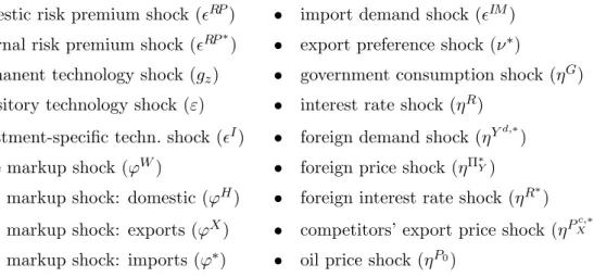
3.2.2 Shocks 37
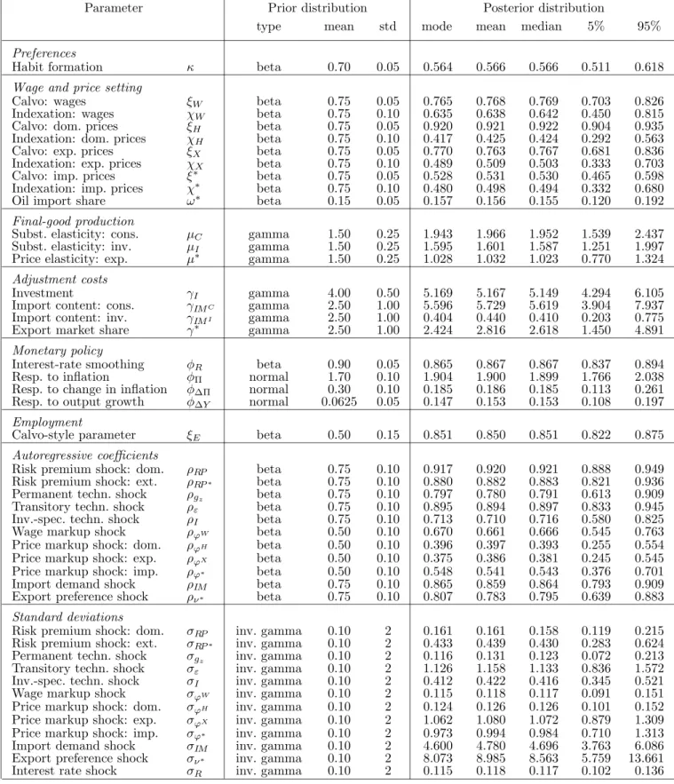
3.3 Calibration and prior distributions 38
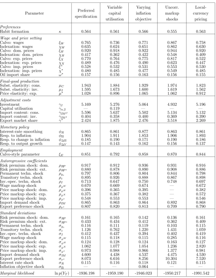
3.3.1 Calibration 38 3.3.2 Prior distributions 39 3.4 Estimation results 41 3.5 Sensitivity analysis 44 4 Model properties 45 4.1 Impulse-response functions 46 4.2 Forecast-error-variance decompositions 48
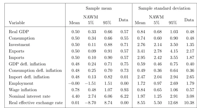
4.3 Implied sample moments 50
4.4 Forecasting performance 51
5 Applications 53
5.1 Historical decompositions 53
5.2 Counterfactual scenarios 55
5.3 Mean and interval predictions 56
5.4 Prediction events 58
6 Conclusion 59
References 61
Appendices 64
Appendix A: The log-linearised model 64
Appendix B: Computation of the steady state 76
Tables and fi gures 82
European Central Bank Working Paper Series 121
Abstract
In this paper, we outline a version of the New Area-Wide Model (NAWM) of the euro area designed for use in the (Broad) Macroeconomic Projection Exercises regularly undertaken by ECB/Eurosystem staff. We present estimation results for the NAWM that are obtained by employing Bayesian inference methods and document the properties of the estimated model by reporting its impulse-response functions and forecast-error-variance decompositions, by inspecting the model-based sample moments, and by examining the model’s forecasting performance relative to a number of benchmarks, including a Bayesian VAR. We finally consider several applications to illustrate the potential contributions the NAWM can make to forecasting and policy analysis.
JEL Classification: C11, C32, E32, E37
Keywords: DSGE modelling, open-economy macroeconomics, Bayesian inference, forecasting, policy analysis, euro area
Non-Technical Summary
This paper reports on the progress made in estimating a version of the New Area-Wide Model (NAWM)—a micro-founded open-economy model of the euro area under devel-opment at the European Central Bank (ECB)—that is designed for use in the (Broad) Macroeconomic Projection Exercises regularly undertaken by ECB/Eurosystem staff and for policy analysis. The NAWM is neo-classical in nature and centred around intertemporal decisions of households and firms which are maximising expected life-time utility and the expected stream of profits, respectively. As a result, forward-looking expectations play a key role in influencing the adjustment dynamics of both quantities and prices, and changes in supply-side factors have a pronounced impact already in the short run. At the same time, the NAWM includes a number of nominal and real frictions that have been identified as empirically important, such as sticky prices and wages (so that some Keynesian features prevail in the short run), habit persistence in consumption and adjustment costs in invest-ment. Moreover, it incorporates analogous frictions relevant in an open-economy setting, including local-currency pricing (giving rise to imperfect exchange-rate pass-through in the short run), and costs of adjusting trade flows.
The design of the NAWM for use in the ECB/Eurosystem staff projections has been guided by two important considerations, namely (i) to provide a comprehensive set of core projection variables and (ii) to allow conditioning on monetary, fiscal and external devel-opments which, in the form of technical assumptions, are an important element of the projections. As a consequence, the scale of the model—compared with a typical DSGE model—is relatively large. Employing Bayesian methods, it is estimated on 18 key macroe-conomic variables, including real GDP, private consumption, total investment, government consumption, exports and imports, a number of deflators, employment and wages, and the short-term nominal interest rate. In addition, data for the nominal effective exchange rate, euro area foreign demand, euro area competitors’ export prices as well as oil prices are used, which are deemed important variables in the projections capturing the influence of external developments. Conformable with the number of variables, 18 structural shocks are consid-ered in the estimation. These shocks are latent factors with an economic interpretation that help typifying the sources of the observed fluctuations in the data.
The use of Bayesian methods for estimating the NAWM enables us to assess the data coherence of the model as a whole and to compare alternative, not necessarily nested spec-ifications of the model. Another advantage of using Bayesian methods is that it allows us to construct probability distributions for the model’s parameters and for model-based
fore-casts, and to thereby quantify the uncertainty associated with model-based analysis and forecasting. This probabilistic approach also extends to validating the properties of the model economically by assessing the propagation of its structural shocks (on the basis of the model’s impulse-response functions), the contribution of the structural shocks to the observed fluctuations in the variables used in the estimation (forecast-error-variance de-compositions), and the implied sample moments for these variables (unconditional means, standard deviations and correlations). It also permits comparing the model’s out-of sample forecast performance (as measured by its root-mean-squared forecast errors) with that of alternative benchmarks, including Bayesian VARs.
All in all, this paper shows that the NAWM fares quite well along these dimensions, and therefore the model seems well suited for forecasting and policy analysis. This is illustrated by a number of applications that, inter alia, exemplify how the NAWM can aid in under-standing the evolution of the euro area economy by interpreting historical developments in terms of its structural shocks and by conducting scenarios that are concerned with coun-terfactual economic events. It is also demonstrated how to use the NAWM for constructing interval forecasts and to analyse the influence of conditioning information.
1
Introduction
Recent years have witnessed the development of a new generation of dynamic stochastic general equilibrium (DSGE) models that build on explicit micro-foundations with optimising agents. Major advances in estimation methodology allowed estimating variants of these models that are able to compete, in terms of data coherence, with more standard time-series models, such as vector autoregressions.1 Accordingly, the new generation of micro-founded DSGE models provides a framework that appears particularly suited for evaluating the consequences of alternative macroeconomic policies. More recently, increasing efforts have been undertaken to use these models also for forecasting.2
Against this background, this paper reports on the progress made in estimating a version of the New Area-Wide Model (NAWM)—a micro-founded open-economy model of the euro area under development at the European Central Bank (ECB)—that is designed for use in the (Broad) Macroeconomic Projection Exercises regularly undertaken by ECB/Eurosystem staff.3 The estimated version of the NAWM complements a calibrated version—richer in
detail and open for topic-driven extensions—that has been developed for analysing a broader range of policy issues in a flexible manner (cf. Coenen, McAdam and Straub, 2007).4 In pursuing this parallel development strategy, the NAWM builds extensively on the earlier work by Smets and Wouters (2003) and Adolfson, Las´een, Lind´e and Villani (2007), who estimated, respectively, a closed and a small-open economy model of the euro area using Bayesian techniques. Moreover, the NAWM also draws on the advances made in developing the International Monetary Fund’s calibrated Global Economy Model (GEM; cf. Bayoumi, Laxton and Pesenti, 2004) and the Federal Reserve Board’s calibrated open-economy model named SIGMA (cf. Erceg, Guerrieri and Gust, 2006).
1
See, among others, Smets and Wouters (2003, 2007), del Negro, Schorfheide, Smets and Wouters (2007), and Adolfson, Lind´e, Las´een and Villani (2007), who estimate, using Bayesian methods, variants of the model by Christiano, Eichenbaum and Evans (2005).
2See Smets and Wouters (2004), Adolfson, Andersson, Lind´e, Villani and Vredin (2007), Adolfson, Lind´e
and Villani (2007), and Edge, Kiley and Laforte (2008).
3
In connection with the NAWM project, a Matlab program for Bayesian estimation and evaluation of DSGE and vector autoregressive models has been developed (cf. Warne, 2008). This program is named YADA (Yet Another DSGE Application) and available upon request.
4For applications that focus on fiscal policy issues see Coenen and McAdam (2006), Coenen, McAdam
The NAWM succeeds the Area-Wide Model (AWM; cf. Fagan, Henry and Mestre, 2001), which is a traditional macroeconomic model of the euro area that has been extensively used at the ECB over the past ten years. There are notable differences between the two models. The NAWM is neo-classical in nature and centred around intertemporal decisions of house-holds and firms which are maximising expected life-time utility and the expected stream of profits, respectively. As a result, forward-looking expectations play a key role in influencing the adjustment dynamics of both quantities and prices, and changes in supply-side factors have a pronounced impact already in the short run. At the same time, the NAWM includes a number of nominal and real frictions that have been identified as empirically important, such as sticky prices and wages (so that some Keynesian features prevail in the short run), habit persistence in consumption and adjustment costs in investment. Moreover, it incor-porates analogous frictions relevant in an open-economy setting, including local-currency pricing (giving rise to imperfect exchange-rate pass-through in the short run), and costs of adjusting trade flows. In contrast, the AWM features predominantly Keynesian behaviour in the short run, even though it has a basic neo-classical steady state. Thus, supply-side effects consistent with profit maximisation materialise only in the long run. The short-run dynamics of aggregate supply and aggregate demand are not explicitly derived from an optimisation framework, but instead specified and estimated in an ad hoc error-correction form. For this reason, and because of the absence of an explicit treatment of expectations, quantities and prices tend to adjust only very sluggishly.
The development of the estimated version of the NAWM has been guided by two impor-tant considerations, namely (i) to provide a comprehensive set of core projection variables and (ii) to allow conditioning on monetary, fiscal and external developments which, in the form of technical assumptions, are an important element of the ECB/Eurosystem staff projections.5 As a consequence, the scale of the model—compared with a typical DSGE model—is relatively large. Employing Bayesian methods, it is estimated on 18 key macroe-conomic variables, including real GDP, private consumption, total investment, government consumption, exports and imports, a number of deflators, employment and wages, and the short-term nominal interest rate. In addition, we utilise data on the nominal effective
5For an overview of the projection exercises and a description of the techniques and tools used therein,
exchange rate, euro area foreign demand, euro area competitors’ export prices as well as oil prices, which are deemed important variables in the projections capturing the influ-ence of external developments.6 As a novel feature, we use the recently compiled extra-euro area trade data (both volumes and prices) which appears economically more compelling than the use of total trade data. Conformable with the number of variables, 18 structural shocks are considered in the estimation. These shocks are latent factors with an economic interpretation that help typifying the sources of the observed fluctuations in the data.
Compared with the calibrated version of the NAWM, which consists of two symmetric countries representing the euro area and the rest of the industrialised world, the estimated version maintains the simplifying assumption that the euro area is a small open economy, motivated by the aforementioned fact that the ECB/Eurosystem staff projections are made conditional on assumptions regarding external developments. Moreover, to ease the es-timation of the model, the fiscal sector has been simplified by assuming that Ricardian equivalence holds. In this context, the assumption that a fraction of households is limited in their ability to participate in asset markets has been abandoned, along with the usage of money as a means of facilitating transactions. In contrast, the estimated version has been augmented by including a unit-root technology to account for a common stochastic trend in real quantities. We also explore the importance of allowing for a possibly time-varying in-flation objective to capture the nominal convergence process in the run up to the formation of the European Economic and Monetary Union (EMU).
The use of Bayesian inference methods for estimating the NAWM enables us to assess the data coherence of the model as a whole and to compare alternative, not necessarily nested specifications of the model. Another advantage of using Bayesian methods is that it allows us to construct probability distributions for the model’s parameters and for model-based forecasts, and to thereby quantify the uncertainty associated with model-based analysis and forecasting. This probabilistic approach also extends to validating the properties of the model economically by assessing the propagation of its structural shocks (on the basis of the model’s impulse-response functions), the contribution of the structural shocks to
6The version of the NAWM actually used in the projections has been extended by bridge equations for
HICP excluding energy and HICP energy, the latter measuring the direct impact of changes in oil prices on the HICP, as well as a number of other macroeconomic variables, including unemployment.
the observed fluctuations in the variables used in the estimation (forecast-error-variance decompositions), and the implied sample moments for these variables (unconditional means, standard deviations and correlations). It also permits comparing the model’s out-of sample forecast performance (as measured by its root-mean-squared forecast errors) with that of alternative benchmarks, including Bayesian VARs.
All in all, this paper shows that the NAWM fares quite well along these dimensions, and therefore the model seems well suited for forecasting and policy analysis. This is illustrated by a number of applications that, inter alia, exemplify how the NAWM can aid in under-standing the evolution of the euro area economy by interpreting historical developments in terms of its structural shocks and by conducting scenarios that are concerned with coun-terfactual economic events. It is also demonstrated how to use the NAWM for constructing interval forecasts and to analyse the influence of conditioning information.
The remainder of the paper is organised as follows. Section 2 outlines the NAWM for forecasting and policy analysis, while Section 3 presents our estimation results, along with some sensitivity analysis. Section 4 documents the properties of the estimated model, whereas Section 5 considers several applications. Section 6 concludes and discusses direc-tions for future extensions. Two appendices provide details on the log-linear version of the model and the computation of its steady state.
2
Model Specification
Within the euro area—henceforth, domestic—economy, there are four types of economic agents: households, firms, a fiscal authority, and a monetary authority. As regards firms, we distinguish between producers of tradable differentiated intermediate goods and produc-ers of three non-tradable final goods: a private consumption good, a private investment good, and a public consumption good. In addition, there are foreign intermediate-good producers that sell their differentiated goods in domestic markets, and a foreign retail firm that combines the exported domestic intermediate goods. International linkages arise from the trade of intermediate goods and international assets, allowing for limited exchange-rate pass-through on the import side and imperfect risk sharing.
In the following, we describe the behaviour of the different types of agents, formulate the market-clearing conditions and the aggregate resource constraint, and state the law of motion for the domestic (net) holdings of foreign assets. In this context, we also define expressions for the trade balance and the terms of trade. To the extent needed, foreign variables and parameters are indexed with an asterisk, ‘∗’.
2.1 Households
There is a continuum of households indexed byh∈[ 0,1 ], the instantaneous utility of which depends on the level of consumption as well as hours worked. Each household accumulates physical capital, the services of which it rents out to firms, and buys and sells domestic government bonds as well as internationally traded foreign bonds. This enables households to smooth their consumption profile in response to shocks. The households supply dif-ferentiated labour services to firms and act as wage setters in monopolistically competitive markets. As a consequence, each household is committed to supply sufficient labour services to satisfy firms’ labour demand.
Preferences and Constraints
Each household h maximises its lifetime utility in a given period t by choosing purchases of the consumption good, Ch,t, purchases of the investment good, Ih,t, which determines
next period’s physical capital stock, Kh,t+1, the intensity with which the existing capital
stock is utilised in production,uh,t, and next period’s (net) holdings of domestic government
bonds and internationally traded foreign bonds, Bh,t+1 and Bh,t∗ +1, respectively, given the
following lifetime utility function:
Et " ∞ X k=0 βk ǫCt+kln (Ch,t+k−κ Ct+k−1)− ǫN t+k 1 +ζ (Nh,t+k) 1+ζ ! # , (1)
where β denotes the discount factor and ζ is the inverse of the Frisch elasticity of labour supply.7 The parameterκmeasures the degree of external habit formation in consumption. Thus, the utility of household h depends positively on the difference between the current level of individual consumption, Ch,t, and the lagged economy-wide consumption level,
7
In contrast to the calibrated version of the NAWM, the utility function is assumed to be logarithmic in consumption in accordance with the balanced-growth property of the model.
Ct−1, and negatively on the number of hours worked, Nh,t. We will refer to ǫCt and ǫNt as
consumption preference and labour-supply shocks, respectively.
Household h faces the following period-by-period budget constraint: (1 +τtC)PC,tCh,t+PI,tIh,t + (ǫRPt Rt)−1Bh,t+1+ ((1−ΓB∗(sB∗,t+1;ǫRP ∗ t ))Rt∗)−1StBh,t∗ +1+ Υh,t+ Ξt = (1−τtN −τWh t ) Wh,tNh,t+ (1−τtK) (RK,tuh,t−Γu(uh,t)PI,t)Kh,t +τtKδ PI,tKh,t+ (1−τtD)Dh,t−Tt+Bh,t+StBh,t∗ , (2)
where PC,t and PI,t are the prices of a unit of the private consumption good and the
investment good, respectively. Nh,t denotes the labour services provided to firms at wage
rate Wh,t; RK,t indicates the rental rate for the effective capital services rented to firms, uh,tKh,t, andDh,t are the dividends paid by the household-owned firms. Rt andRt∗ denote
the respective risk-less returns on domestic government bonds and internationally traded foreign bonds. The latter are denominated in foreign currency and, thus, their domestic value depends on the nominal exchange rateSt (expressed in terms of units of the domestic
currency per unit of the foreign currency).
The fiscal authority absorbs part of the household’s gross income to finance its expen-diture. In this context, τC
t denotes the consumption tax rate levied on the household’s
consumption purchases; andτN
t ,τtK andτtD are the tax rates levied on the different sources
of the household’s income: wage income,Wh,tNh,t, capital income, RK,tKh,t, and dividend
income, Dh,t.8 Here, for simplicity, we assume that the utilisation cost of physical capital
as well as physical capital depreciation,δ PI,tKh,t, are exempted from taxation. τtWh is the
additional payroll tax rate levied on wage income (representing the household’s contribution to social security). The term Tt denotes lump-sum taxes.
The effective return on the risk-less domestic bonds depends on a financial interme-diation premium, represented by the exogenous “risk premium” shock ǫRP
t , which drives
a wedge between the interest rate controlled by the monetary authority and the
re-8
turn required by the household.9 Similarly, when taking a position in the international bond market, the household encounters an external financial intermediation premium ΓB∗(sB∗,t+1;ǫRP
∗
t ) which depends on the economy-wide (net) holdings of internationally
traded foreign bonds expressed in domestic currency relative to domestic nominal output,
sB∗,t+1 =StBt∗
+1/PY,tYt, and takes the form:
ΓB∗(sB∗,t+1;ǫRP ∗ t ) = γB∗ ǫRPt ∗ 1 γB∗ exp StB ∗ t+1 PY,tYt ! −1 ! (3) with γB∗ >0.10 That is, if the domestic economy is a net debtor, households have to pay an increasing external intermediation premium on their international debt. The shockǫRP∗
t
represents the exogenous component of the external intermediation premium and will be referred to as external risk premium shock.11 This specification implies that, in the non-stochastic steady state, households have no incentive to hold foreign bonds and the econ-omy’s net foreign asset position is zero. The incurred intermediation premium is rebated in a lump-sum manner, being indicated by Ξt.
For analytical convenience, each household h is assumed to hold state-contingent secu-rities, Υh,t. These securities are traded amongst households and provide insurance against
household-specific wage-income risk. This guarantees that the marginal utility of consump-tion out of wage income is identical across households.12 As a result, all households will choose identical allocations in equilibrium.13
The physical capital stock owned by household h evolves according to the following capital accumulation equation:
Kh,t+1 = (1−δ)Kh,t+ǫIt(1−ΓI(Ih,t/Ih,t−1))Ih,t, (4)
where δ is the depreciation rate, ΓI(Ih,t/Ih,t−1) represents a generalised adjustment cost
function formulated in terms of the (gross) rate of change in investment, Ih,t/Ih,t−1, andǫIt 9See Smets and Wouters (2007) for further discussion.
10
Note that we have used current nominal output and the current exchange rate to scaleB∗
t+1, because
the net foreign asset position is a predetermined variable.
11
The exponential weighing of the external risk premium shock implies that the shock enters the log-linearised version of the intermediation premium with a unit coefficient.
12
The existence of state-contingent securities renders the model tractable under staggered wage setting when households are supplying differentiated labour services.
denotes an investment-specific technology shock affecting the efficiency of the newly installed investment good. The adjustment cost function is assumed to take the following form:
ΓI(Ih,t/Ih,t−1) = γI 2 Ih,t Ih,t−1 −gz !2 (5) with γI > 0. The term gz denotes the economy’s trend growth rate in the non-stochastic
steady state.
Finally, as regards the provision of effective capital services, varying the intensity of utilising the physical capital stock, uh,t, is subject to a proportional cost Γu(uh,t) which is
assumed to take the following form:
Γu(uh,t) = γu,1(uh,t−1) + γu,2 2 (uh,t−1) 2 (6) withγu,1, γu,2 >0. Choice of Allocations
Defining as Λh,t/PC,t and Λh,tQh,t the Lagrange multipliers associated with the budget
con-straint (2) and the capital accumulation equation (4), respectively, the first-order conditions for maximising the household’s lifetime utility function (1) with respect toCh,t,Ih,t,Kh,t+1, uh,t,Bh,t+1 and Bh,t∗ +1 are given by:
Λh,t = ǫCt (Ch,t−κ Ct−1)−1 1 +τC t , (7) PI,t PC,t = Qh,tǫIt 1−ΓI(Ih,t/Ih,t−1)−Γ′I(Ih,t/Ih,t−1) Ih,t Ih,t−1 ! (8) +βEt " Λh,t+1 Λh,t Qh,t+1ǫIt+1Γ′I(Ih,t+1/Ih,t) Ih,t2 +1 Ih,t2 # , Qh,t = βEt " Λh,t+1 Λh,t (1−δ)Qh,t+1 (9) + (1−τtK+1) RK,t+1 PC,t+1 uh,t+1+ τtK+1δ−(1−τtK+1) Γu(uh,t+1) PI,t+1 PC,t+1 # , RK,t = Γ′u(uh,t)PI,t, (10) β ǫRPt RtEt " Λh,t+1 Λh,t PC,t PC,t+1 # = 1, (11)
β(1−ΓB∗(sB∗,t+1;ǫRP ∗ t ))R∗tEt " Λh,t+1 Λh,t PC,t PC,t+1 St+1 St # = 1. (12)
Here, Λh,t represents the shadow price of a unit of the consumption good; that is, the
marginal utility of consumption out of income. Similarly, Qh,t measures the shadow price
of a unit of the investment good; that is, Tobin’sQ.14
In equilibrium, with all households choosing identical allocations, the combination of the first-order conditions with respect to the holdings of domestic and internationally traded bonds, (11) and (12), yields a risk-adjusted uncovered interest parity (UIP) condition, reflecting the assumption that the return on internationally traded bonds is subject to an external financial intermediation premium.
Wage Setting
Each household h supplies its differentiated labour services Nh,t in monopolistically
com-petitive markets. There is sluggish wage adjustment due to staggered wage contracts `a la Calvo (1983). Accordingly, householdh receives permission to optimally reset its nominal wage contract Wh,t in a given periodtwith probability 1−ξW.
All households that receive permission to reset their wage contracts in a given period t
choose the same wage rate ˜Wt= ˜Wh,t. Those households which do not receive permission are
allowed to adjust their wage contracts to productivity developments and inflation according to the following scheme:
Wh,t = gz,t Π†C,tWh,t−1, (13)
wheregz,t represents the (gross) rate of underlying labour productivity growth and Π†C,t=
ΠχW
C,t−1Π¯ 1−χW
t is a geometric average of past (gross) consumer price inflation, ΠC,t−1 = PC,t−1/PC,t−2, and the monetary authority’s possibly time-varying (gross) inflation
objec-tive, ¯Πt. The weight of past inflation is determined by the indexation parameter χW.
Each householdh receiving permission to reset its wage contract in periodt maximises its lifetime utility function (1) subject to its budget constraint (2), the demand for its differentiated labour services (the formal derivation of which we postpone until we consider
14
We note that the domestic risk premium shock, ǫRP
t , affects investment via Tobin’s Q and helps to
explain the co-movement of consumption and investment observed in the data. In contrast, the consumption preference shock,ǫC
the decision problem of the domestic intermediate-good firms in Section 2.2.1) and the wage-indexation scheme (13).
Hence, we obtain the following first-order condition characterising the households’ op-timal wage-setting decision:
Et ∞ X k=0 (ξWβ)k Λt+k(1−τtN+k−τ Wh t+k)gz;t,t+k Π†C;t,t+k ΠC;t,t+k ˜ Wt PC,t (14) −ϕWt+kǫNt+k(Nh,t+k)ζ ! Nh,t+k # = 0,
where Λt+k denotes the marginal utility out of income (equal across all households),
gz;t,t+k =Qks=1gz,t+s, Π†C;t,t+k= Qk s=1Π χ W C,t+s−1Π¯ 1−χ W t+s and ΠC;t,t+k =Qks=1ΠC,t+s−1.
This expression states that in those labour markets in which wage contracts are re-optimised, the latter are set so as to equate the households’ discounted sum of expected after-tax marginal revenues, expressed in consumption-based utility terms, Λt+k, to the
dis-counted sum of expected marginal cost, expressed in terms of marginal disutility of labour, ∆h,t+k =−Nh,tζ +k. In the absence of wage staggering (ξW = 0), the factor ϕWt represents
a possibly time-varying markup of the real after-tax wage charged over the households’ marginal rate of substitution between consumption and leisure,
(1−τtN −τWh t ) ˜ Wt PC,t = −ϕWt ǫNt ∆t Λt , (15)
reflecting the existence of monopoly power on the part of the households.15
Aggregate Wage Dynamics
With the continuum of households setting the wage contracts for their differentiated labour services on the basis of equation (13) and equation (14), respectively, the aggregate wage indexWt(see Section 2.2.1 for details) evolves according to
Wt = ξW gz,tΠ†C,tWt−1 1 1−ϕW t + (1−ξ W) ˜ Wt 1 1−ϕW t !1−ϕW t . (16) 2.2 Firms
There are two types of monopolistically competitive intermediate-good firms: A continuum of domestic intermediate-good firms indexed by f ∈ [ 0,1 ] which produce differentiated
15
Here we have used the fact that, in equilibrium, the marginal disutility is equal across households; that is ∆h,t= ∆t.
outputs that are sold domestically or abroad, and a continuum of foreign intermediate-good firms indexed by f∗ ∈ [ 0,1 ] which produce differentiated outputs that are sold in
domes-tic markets. In addition there is a set of three representative domesdomes-tic final-good firms which combine the purchases of domestically-produced intermediate goods with purchases of imported intermediate goods into three distinct non-tradable goods, namely a private con-sumption good, a private investment good and a public concon-sumption good. Finally, there is a representative foreign retail firm that combines the exported domestic intermediate goods.
2.2.1 Domestic Intermediate-Good Firms
Technology
Each domestic intermediate-good firm f produces a differentiated intermediate good Yf,t
with an increasing-returns-to-scale Cobb-Douglas technology that is subject to fixed costs of production,ztψ, Yf,t = max h εt(Kf,ts )α(ztNf,t)1−α−ztψ,0 i , (17)
utilising as inputs homogenous capital services, Ks
f,t, that are rented from households in
fully competitive markets, and an index of differentiated labour services,Nf,t, which
com-bines household-specific varieties of labour that are supplied in monopolistically competitive markets, Nf,t = Z 1 0 Nf,th 1 ϕW t dh !ϕWt . (18)
Here, the possibly time-varying parameterϕW
t >1 is inversely related to the intratemporal
elasticity of substitution between the differentiated labour services supplied by the house-holds,ϕW
t /(ϕWt −1)>1. As shown above, the parameter ϕWt has a natural interpretation
as a markup in the household-specific labour market.16
The variable εt represents a serially correlated, but transitory technology shock that
affects total-factor productivity, while the variableztdenotes apermanenttechnology shock
shifting the productivity of labour lastingly. The permanent technology shock introduces
16
Note that the exposition of the calibrated version of the NAWM is centred around the intratemporal elasticity of substitution which is assumed to be time invariant.
a unit root in the firms’ output and evolves according to the following serially correlated process,
gz,t = (1−ρgz)gz+ρgzgz,t−1+η
gz
t , (19)
where gz,t=zt/zt−1 represents the (gross) rate of labour-augmenting productivity growth
with steady-state valuegz.
Both technology shocks, and the fixed costs of production, are assumed to be identical across firms. The fixed costs are scaled by the permanent technology shock to guarantee that fixed costs as a fraction of output do not vanish as output grows.17
Capital and Labour Inputs
Taking the rental cost of capital RK,t and the aggregate wage index Wt as given, the
intermediate-good firm’s optimal demand for capital and labour services solves the problem of minimising total input cost RK,tKf,t+ (1 +τ
Wf
t )WtNf,t subject to the technology
con-straint (17). Here,τWf
t denotes the payroll tax rate levied on wage payments (representing
the firm’s contribution to social security).
Defining as MCf,t the Lagrange multiplier associated with the technology constraint
(17), the first-order conditions of the firm’s cost minimisation problem with respect to capital and labour inputs are given, respectively, by
αYf,t+ztψ Ks f,t MCf,t = RK,t, (20) (1−α)Yf,t+ztψ Nf,t MCf,t = (1 +τ Wf t )Wt, (21)
or, more compactly,
α 1−α Nf,t Ks f,t = RK,t (1 +τWf t )Wt . (22)
Here, the Lagrange multiplier MCf,t measures the shadow price of varying the use of
capital and labour services; that is, nominal marginal cost. We note that, since all firmsf
face the same input prices and since they all have access to the same production technology, nominal marginal cost MCf,t are identical across firms; that is, MCf,t=MCt with
MCt = 1 εtzt1−ααα(1−α)1−α (RK,t)α((1 +τ Wf t )Wt)1−α. (23) 17
The parameter ψ will be chosen to ensure zero profits in steady state. This in turn guarantees that there is no incentive for other firms to enter the market in the long run.
With the nominal wage contract Wh,t for the differentiated labour services of household hbeing set in monopolistically competitive markets, firmf takesWh,t as given and chooses
the optimal input of each labour varietyhby minimising the total wage-related labour cost R1
0 Wh,tNf,th dh, subject to the aggregation constraint (18).
The resulting demand for labour variety h is a function of the household-specific wage rate Wh,t relative to the aggregate wage indexWt:
Nf,th = W h,t Wt − ϕWt ϕW t −1 N f,t (24) withϕW
t /(ϕWt −1) representing the wage elasticity of labour demand.
The wage indexWtcan be obtained by substituting the labour index (18) into the labour
demand schedule (24) and then integrating over the continuum of households:
Wt = Z 1 0 W 1 1−ϕW t h,t dh !1−ϕWt . (25)
Aggregating over the continuum of firms, we obtain the following aggregate demand for the labour services of a given household h:
Nth = Z 1 0 Nf,th df = W h,t Wt − ϕWt ϕW t −1 N t. (26) Price Setting
Each firmf sells its differentiated outputYf,t in both domestic and foreign markets under
monopolistic competition. We assume that the firm charges different prices at home and abroad, setting prices in producer (that is, domestic) currency regardless of the market of destination.18 In both markets, there is sluggish price adjustment due to staggered price contracts `a la Calvo (1983). Accordingly, firmf receives permission to optimally reset prices in a given period teither with probability 1−ξH or with probability 1−ξX, depending on whether the firm sells its differentiated output in the domestic or the foreign market.
Defining as PH,f,t the domestic price of goodf and asPX,f,t its foreign price, all firms
that receive permission to reset their price contracts in a given period t choose the same
18This contrasts with the assumption of local-currency pricing that is maintained in the calibrated version
of the NAWM for goods that are sold abroad. As shown in the sensitivity analysis in Section 3.5, producer-currency pricing is strongly preferred by the data.
price, ˜PH,t= ˜PH,f,t and ˜PX,t= ˜PX,f,t, depending on the market of destination. Those firms
which do not receive permission are allowed to adjust their prices according to the following schemes: PH,f,t = Π χ H H,t−1Π¯ 1−χ H t PH,f,t−1, (27) PX,f,t = Π χX X,t−1Π¯ 1−χX t PX,f,t−1. (28)
That is, the price contracts are indexed to a geometric average of past (gross) intermediate-good inflation, ΠH,t−1 = PH,t−1/PH,t−2 and ΠX,t−1 = PX,t−1/PX,t−2, and the possibly
time-varying (gross) inflation objective of the domestic monetary authority, ¯Πt, where χH
and χX are indexation parameters determining the weight on past inflation.
Each firmf receiving permission to optimally reset its domestic and/or foreign price in periodtmaximises the discounted sum of its expected nominal profits,
Et " ∞ X k=0 Λt,t+k ξHk DH,f,t+k+ξXk DX,f,t+k # , (29)
subject to the price-indexation schemes (27) and (28) and taking as given domestic and foreign demand for its differentiated output,Hf,t and Xf,t (to be derived in Sections 2.2.3
and 2.2.4). The stochastic discount factor Λt,t+k can be obtained from the consumption
Euler equation of the households, and
DH,f,t = PH,f,tHf,t−MCtHf,t, (30)
DX,f,t = PX,f,tXf,t−MCtXf,t (31)
are period-tnominal profits (net of fixed costs) yielded in the domestic and foreign markets, respectively, which are distributed as dividends to the households.19 Hence, we obtain the following first-order condition characterising the firm’s optimal pricing decision for its output sold in the domestic market:
Et "∞ X k=0 ξk HΛt,t+k Π†H,t,t+kP˜H,t−ϕHt+kMCt+k Hf,t+k # = 0, (32)
where we have substituted the indexation scheme (27), noting thatPH,f,t+k= Π†H,t,t+kP˜H,t
with Π†H,t,t+k =Qks=1ΠχH
H,t+s−1Π¯ 1−χH t+s .
19Note that we have made use of the first-order conditions (9) and (21) to derive the expressions for
This expression states that in those intermediate-good markets in which price contracts are re-optimised, the latter are set so as to equate the firm’s discounted sum of expected revenues to the discounted sum of expected marginal cost. In the absence of price staggering (ξH = 0), the factor ϕH
t represents a possibly time-varying markup of the price charged in
domestic markets over nominal marginal cost, reflecting the degree of monopoly power on the part of the intermediate-good firm.
Similarly, we obtain the following first-order condition characterising the firm’s optimal pricing decision for its output sold in the foreign market:
Et "∞ X k=0 ξXk Λt,t+k Π†X,t,t+kP˜X,t−ϕXt+k MCt+k Xf,t+k # = 0, (33)
where we have substituted the indexation scheme (28), noting thatPX,f,t+k= Π†X,t,t+kP˜X,t
with Π†X,t,t+k =Qks=1ΠχX
X,t+s−1Π¯ 1−χX t+s .
Aggregate Price Dynamics
With the continuum of intermediate-good firms setting the price contracts for their dif-ferentiated products sold domestically on the basis of equation (27) and equation (32), respectively, the aggregate price indexPH,t (see Section 2.2.3) evolves according to
PH,t = (1−ξH)( ˜PH,t) 1 1−ϕH t +ξ H ΠχH H,t−1Π¯ 1−χH t PH,t−1 1 1−ϕH t !1−ϕH t . (34)
A similar relationship holds for the aggregate index of price contracts set for the differ-entiated products sold abroad (see Section 2.2.4) with
PX,t = (1−ξX)( ˜PX,t) 1 1−ϕX t +ξ X ΠχX X,t−1Π¯ 1−χX t PX,t−1 1 1−ϕX t !1−ϕX t . (35)
2.2.2 Foreign Intermediate-Good Firms
Each foreign intermediate-good firmf∗ sells its differentiated goodY∗
f∗,t in domestic market under monopolistic competition, setting the price in local (that is, domestic) currency, as in Betts and Devereux (1996). Again, there is sluggish price adjustment due to staggered price contracts `a la Calvo. Accordingly, the foreign intermediate-good firm, or exporter, receives permission to optimally reset its price in a given period t with probability 1−ξ∗
and has access to the following indexation scheme with parameter χ∗: PIM,f∗,t = Πχ ∗ IM,t−1Π¯ 1−χ∗ t PIM,f∗,t−1, (36)
where PIM,f∗,t =PX,f∗ ∗,t and ΠIM,t−1 =PIM,t−1/PIM,t−2 with PIM,t =PX,t∗ . Here, we have
utilised the fact that, with foreign exporters setting prices in domestic currency, the price of the intermediate good imported from abroad (the import price index of the home country) is equal to the price charged by the foreign exporter in the home country (the export price index of the foreign country).
Each foreign exporter f∗ receiving permission to optimally reset its price in period t
maximises the discounted sum of its expected nominal profits, Et " ∞ X k=0 (ξ∗)kΛ∗t,t+kD∗f∗,t+k/St+k # , (37)
subject to the price-indexation scheme and the domestic (import) demand for its differen-tiated output,IMf∗,t=X∗
f∗ (to be derived in Sections 2.2.3), where
Df∗∗,t = PIM,f∗,tIMf∗,t−MCt∗IMf∗,t (38) with MC∗ t = St(PO,t)ω ∗ (P∗ Y,t)1−ω ∗
representing the foreign exporter’s nominal marginal cost. The latter is defined as a simple geometric average of the price of oil,PO,t, and foreign
prices,P∗
Y,t, with ω∗ measuring the share of oil in imports.
Hence, we obtain the following first-order condition characterising the foreign exporter’s optimal pricing decision for its output sold in the domestic market:
Et "∞ X k=0 (ξ∗)kΛ∗t,t+kΠ†IM,t,t+kP˜IM,t−ϕ∗t+kMCt∗+k IMf∗,t+k/St+k # = 0, (39)
where we have substituted the indexation scheme (36), noting that PIM,f∗,t+k = Π†
IM,t,t+k
˜
PIM,t with Π†IM,t,t+k =
Qk s=1Π χ∗ IM,t+s−1Π¯ 1−χ∗ t+s .
The associated aggregate index of price contracts for the differentiated products sold in domestic markets (see Section 2.2.3) evolves according to
PIM,t = (1−ξ∗)( ˜PIM,t) 1 1−ϕ∗ t +ξ∗ ΠIM,tχ∗ −1Π¯t1−χ∗PIM,t−1 1 1−ϕ∗ t 1−ϕ∗ t . (40)
2.2.3 Domestic Final-Good Firms
There are three different types of final-good firms which combine the purchases of the domestically-produced intermediate goods with purchases of the imported intermediate goods into three distinct non-tradable final goods, namely a private consumption good,
QC
t , a private investment good,QIt, and a public consumption good,QGt .
The representative firm producing the non-tradable final private consumption good,
QC
t , combines purchases of a bundle of domestically-produced intermediate goods, HtC,
with purchases of a bundle of imported foreign intermediate goods,IMC
t , using a
constant-returns-to-scale CES technology,
QCt = ν 1 µC C,t HC t 1−µC1 + (1−νC,t) 1 µC (1−ΓIMC(IMtC/QCt;ǫIMt ))IMtC 1− 1 µC ! µC µC−1 (41) whereµC denotes the intratemporal elasticity of substitution between the distinct bundles
of domestic and foreign intermediate goods, while the possibly time-varying parameterνC,t
measures the home bias in the production of the consumption good.
The final-good firm incurs a cost ΓIMC(IMtC/QCt ;ǫIMt ) when varying the use of the
bundle of imported goods in producing the consumption good, ΓIMC(IMtC/QCt ;ǫIMt ) = γIMC 2 ǫIMt − 1 γIM C IM C t /QCt IMC t−1/QCt−1 −1 !2 (42) withγIMC >0. As a result, the import share is relatively unresponsive in the short run to
changes in the relative price of the bundle of imported goods, while the level of imports is permitted to jump in response to changes in overall demand.20 We will refer to ǫIM
t as an
import demand shock. Defining asHC
f,tandIMfC∗,tthe use of the differentiated output produced by the domestic intermediate-good firmf and the differentiated output supplied by the foreign exporterf∗,
respectively, we have HtC = Z 1 0 Hf,tC 1 ϕH t df !ϕH t , (43) IMtC = Z 1 0 IMfC∗,t 1 ϕ∗ t df∗ ϕ∗ t , (44) 20
While our treatment of the adjustment cost as being external to the firm would formally involve assuming the existence of a large number of firms with appropriate changes in notation (see, e.g., Bayoumi, Laxton and Pesenti, 2004), we abstract from these changes for ease of exposition.
where the possibly time-varying parametersϕH
t , ϕ∗t >1 are inversely related to the
intratem-poral elasticities of substitution between the differentiated outputs supplied by the domestic firms and the foreign exporters, respectively, with ϕHt /(ϕHt −1)>1 and ϕ∗t/(ϕ∗t −1)>1.
As shown above, the parameters ϕH
t and ϕ∗t have a natural interpretation as markups in
the markets for domestic and imported intermediate goods.21
With nominal prices for the differentiated goods f andf∗ being set in monopolistically competitive markets, the final-good firm takes their pricesPH,f,t and PIM,f∗,t as given and chooses the optimal use of the differentiated goodsf andf∗ by minimising the expenditure
for the bundles of differentiated goods,R01PH,f,tHf,tC df and
R1
0 PIM,f∗,tIMfC∗,tdf∗, subject to the aggregation constraints (43) and (44). This yields the following demand equations for the differentiated goods f and f∗:
Hf,tC = PH,f,t PH,t !− ϕHt ϕH t −1 HtC, (45) IMC f∗,t = PIM,f∗,t PIM,t !− ϕ ∗ t ϕ∗ t−1 IMtC, (46) where PH,t = Z 1 0 (PH,f,t) 1 1−ϕH t df !1−ϕHt , (47) PIM,t = Z 1 0 (PIM,f ∗,t) 1 1−ϕ∗ t df∗ 1−ϕ∗t (48) are the aggregate price indexes for the bundles of domestic and imported intermediate goods, respectively.
Next, taking the price indexes PH,t and PIM,t as given, the consumption-good firm
chooses the combination of the domestic and foreign intermediate-good bundles HC
t and
IMC
t that minimises PH,tHtC +PIM,tIMtC subject to aggregation constraint (41). This
yields the following demand equations for the intermediate-good bundles:
HtC = νC,t PH,t PC,t !−µC QCt, (49) IMtC = (1−νC,t) PIM,t PC,tΓ†IMC(IMtC/QCt;ǫIMt ) !−µC QCt 1−ΓIMC(IMtC/QCt;ǫIMt ) , (50) 21
Note that the exposition of the calibrated version of the NAWM is centred around the intratemporal elasticities of substitution which are assumed to be time invariant.
where PC,t = νC,t(PH,t)1−µC + (1−νC,t) PIM,t Γ†IMC(IMtC/QCt ;ǫIMt ) !1−µC 1 1−µC (51) is the price of a unit of the private consumption good and
Γ†IMC(IM
C
t /QCt;ǫIMt ) = 1−ΓIMC(IMtC/QCt;ǫtIM)−Γ′IMC(IMtC/QCt;ǫIMt )IMtC. (52)
The representative firm producing the non-tradable final private investment good,QI t, is
modelled in an analogous manner. Specifically, the firm combines its purchase of a bundle of domestically-produced intermediate goods, HI
t, with the purchase of a bundle of imported
foreign intermediate goods,IMI
t, using a constant-returns-to-scale CES technology,
QIt = ν 1 µI I,t HtI1− 1 µI + (1−ν I,t) 1 µI (1−Γ IMI(IMtI/QtI;ǫIMt ))IMtI 1−1 µI ! µI µI−1 ,(53)
where µI denotes the intratemporal elasticity of substitution between the distinct bundles
of domestic and foreign intermediate inputs, while the possibly time-varying parameterνI,t
measures the home bias in the production of the investment good.
All other variables related to the production of the investment good—import adjustment cost, ΓIMI(IMtI/QIt;ǫIMt ); the optimal demand for firm-specific and bundled domestic and
foreign intermediate goods, HI
f,t,HtI andIMfI∗,t,IMtI, respectively; as well as the price of a unit of the investment good,PI,t—are defined or derived in a manner analogous to that for
the consumption good.22
In contrast, the non-tradable final public consumption good, QG
t , is assumed to be a
composite made only of domestic intermediate goods; that is,QG
t =HtG with HtG = Z 1 0 Hf,tG 1 ϕH t df !ϕH t . (54)
Hence, the optimal demand for the differentiated intermediate good f is given by
Hf,tG = PH,f,t PH,t !− ϕHt ϕH t −1 HtG, (55)
and the price of a unit of the public consumption good isPG,t =PH,t. 22
We note that, even in the absence of import adjustment cost, the prices of the consumption and invest-ment goods may differ due to differences in the home bias parameters.
Aggregating across the three final-good firms, we obtain the following aggregate demand equations for domestic and foreign intermediate goodsf and f∗:
Hf,t = Hf,tC +Hf,tI +Hf,tG = PH,f,t PH,t !− ϕHt ϕH t −1 Ht, (56) IMf∗,t = IMfC∗,t+IMfI∗,t = PIM,f∗,t PIM,t !− ϕ ∗ t ϕ∗ t−1 IMt, (57) whereHt=HtC+HtI+HtG and IMt=IMtC+IMtI.
2.2.4 Foreign Retail Firm
We assume that a representative foreign retail firm combines the purchases of the differen-tiated goods, Xf,t, that are produced by the domestic intermediate-good firms f and sold
abroad, using a CES technology,
Xt = Z 1 0 (Xf,t) 1 ϕX t df !ϕX t , (58)
where the possibly time-varying parameterϕX
t >1 is inversely related to the intratemporal
elasticity of substitution between the differentiated goods supplied by the domestic firms, withϕX
t /(ϕXt −1)>1.
With nominal prices for the exported intermediate goods f being set in producer cur-rency under monopolistic competition, the foreign retailer takes its input pricesPX,f,t/Stas
given and decides on the optimal use of the differentiated inputs by minimising the expen-diture for the bundle of differentiated goods,R01PX,f,t/StXf,tdf, subject to the aggregation
constraint (58).
This yields the following demand equation for the differentiated good f:
Xf,t = PX,f,t PX,t !− ϕXt ϕX t −1 Xt, (59) where PX,t = Z 1 0 (PX,f,t) 1 1−ϕX t df !1−ϕXt (60) is the aggregate price index for the bundle of exported domestic intermediate goods in producer currency.
The retailer takes the aggregate price index PX,t as given and supplies the quantity of
the export bundle, Xt, that satisfies foreign demand. The latter is given by an equation
similar in structure to the domestic import equation,
Xt = νt∗ PX,t/St PX,tc,∗Γ†X(Xt/Ytd,∗;ǫXt ) −µ∗ Ytd,∗ 1−ΓX(Xt/Ytd,∗;ǫXt ) (61) withµ∗denoting the price elasticity of exports. Hereν∗
t represents the possibly time-varying
export share of the domestic intermediate-good firms, which captures the foreign non-price related preferences for domestic goods. The variablePX,tc,∗ denotes the price of foreign firms that are competing with the domestic firms in their export markets, Ytd,∗ is a measure of overall foreign demand, and ΓX(Xt/Ytd,∗;ǫXt ) is an adjustment cost function given by
ΓX(Xt/Ytd,∗;ǫXt ) = γ∗ 2 ǫXt − 1 γ∗ Xt/Ytd,∗ Xt−1/Ytd,−∗1 −1 !2 (62) and Γ†X(Xt/Ytd,∗;ǫXt ) = 1−ΓX(Xt/Ytd,∗;ǫtX)−Γ′X(Xt/Ytd,∗;ǫXt )Xt. (63)
2.3 Fiscal and Monetary Authorities
2.3.1 Fiscal Authority
The fiscal authority purchases the final public consumption good, Gt, issues bonds to
re-finance its outstanding debt, Bt, and raises both distortionary and lump-sum taxes. The
fiscal authority’s period-by-period budget constraint then has the following form:
PG,tGt+Bt = τtCPC,tCt+ (τtN +τtWh) Z 1 0 Wh,tNh,tdh+ τ Wf t WtNt (64) +τtK(RK,tut−(Γu(ut) +δ)PI,t)Kt+τtDDt+Tt+R−t1Bt+1,
where all variables are expressed in economy-wide terms, except for the households’ labour services and wages,Nh,t and Wh,t, which are differentiated across households.
The purchases of the public consumption good Gt are determined exogenously. As
regards the effects of changes in public consumption, we note that “Ricardian equivalence” is assumed to hold. Hence, the particular time path of debt is irrelevant for the households’
choice of allocations. For this reason and without loss of generality, we assume that lump-sum taxes close the fiscal authority’s budget constraint each period. Finally, all distortionary tax rates τtj withj=C, D, K, N, Wh andWf are assumed to be set exogenously.
2.3.2 Monetary Authority
The monetary authority sets the nominal interest rate according to a simple log-linear interest-rate rule,
b
rt = φRrbt−1+ (1−φR) b¯πt+φΠ πbC,t−1−πb¯t+φY ybt (65)
+φ∆Π(πbC,t−bπC,t−1) +φ∆Y (ybt−ybt−1) +ηbtR,
whererbt= log(Rt/R) is the logarithmic deviation of the (gross) nominal interest rate from
its steady-state value. Similarly, πbC,t = log(ΠC,t/Π) denotes the logarithmic deviation of¯
(gross) quarter-on-quarter consumer price inflation ΠC,t =PC,t/PC,t−1 from the monetary
authority’s long-run inflation objective ¯Π, whileπb¯t= log( ¯Πt/Π) represents the logarithmic¯
deviation of the monetary authority’s possibly time-varying inflation objective from its long-run value, which is assumed to follow a serially correlated process with mean zero,
b ¯
πt = ρΠ¯πb¯t−1+ηbΠt¯. (66)
Finally,ybt=Ydt/ztis the logarithmic deviation of aggregate output from the trend output
level implied by the permanent technology shock, which will be referred to as output gap, and ηbR
t is a serially uncorrelated shock to the nominal interest rate.23
2.4 Market Clearing and Aggregate Resource Constraint
In this sub-section, we formulate the various market-clearing conditions which need to hold in equilibrium, along with the aggregate resource constraint.
Market Clearing in the Labour Markets
Each household h acts as wage setter in a monopolistically competitive market. Hence, in
23
In using a trend-based output gap measure we follow Adolfson, Las´een, Lind´e and Villani (2007), whereas Smets and Wouters (2003) employ an output gap concept which is based on the assumption of full price and wage flexibility (cf. Woodford, 2003).
equilibrium the supply of its differentiated labour service needs to equal the intermediate-good firms’ demand,
Nh,t =
Z 1 0
Nf,th df = Nth. (67)
Aggregating over the continuum of householdsh, we have Z 1 0 Nh,tdh = Z 1 0 Nh t dh = Z 1 0 W h,t Wt − ϕWt ϕWt −1 Ntdh = ˇsW,tNt, (68)
where the variable
ˇ sW,t = Z 1 0 W h,t Wt − ϕWt ϕW t −1 dh (69)
measures the degree of wage dispersion across the differentiated labour servicesh.
Given the optimal wage-setting strategies for the households, the measure of wage dis-persion evolves according to
ˇ sW,t = (1−ξW) ˜ Wt Wt !− ϕWt ϕW t −1 +ξW Wt Wt−1 ΠC,t ΠχW C,t−1Π¯ 1−χW t − ϕWt ϕW t −1 ˇ sW,t−1, (70)
where ˜Wtdenotes the optimal wage contract chosen by those households that have received
permission to reset their wages in periodt, and ΠC,t =PC,t/PC,t−1.24
As regards the total wage sum paid by firms to the households, we have Z 1 0 Wh,tNh,tdh = Nt Z 1 0 Wh,t W h,t Wt − ϕWt ϕWt −1 dh = WtNt, (71)
where the first equality has been obtained using the aggregate demand for labour services of variety h, while the last equality uses the properties of the wage index Wt.
Market Clearing in the Capital Market
Market clearing in the rental market for capital services implies that the effective utilisation of capital by households satisfies
utKt = ut Z 1 0 Kh,tdh = Z 1 0 Kf,ts df = Kts. (72) 24
The dispersion term ˇsW,t is equal to one in steady state, and fluctuations in ˇsW,t do vanish in the log-linearised version of the model.
Market Clearing in the Markets for Domestic Intermediate Goods
Each intermediate-good producing firm f acts as price setter in domestic and foreign mo-nopolistically competitive markets. Hence, in equilibrium the supply of its differentiated output needs to equal domestic and foreign demand,
Yf,t = Hf,t+Xf,t. (73)
Aggregating over the continuum of firms f, we obtain the following aggregate resource constraint: Yt = Z 1 0 Yf,tdf = Z 1 0 Hf,tdf + Z 1 0 Xf,tdf = Z 1 0 PH,f,t PH,t !− ϕHt ϕH t −1 Htdf+ Z 1 0 PX,f,t PX,t !− ϕXt ϕX t −1 Xtdf = ˇsH,tHt+ ˇsX,tXt, (74)
where the variables
ˇ sH,t = Z 1 0 PH,f,t PH,t !− ϕHt ϕH t −1 df, (75) ˇ sX,t = Z 1 0 PX,f,t PX,t !− ϕXt ϕX t −1 df (76)
measure the degree of price dispersion across the differentiated goods f sold either domes-tically or abroad.
Given the optimal price-setting strategies for intermediate-good firms, the two measures of price dispersion evolve according to
ˇ sH,t = (1−ξH) ˜ PH,t PH,t !− ϕHt ϕH t −1 +ξH ΠH,t ΠχH H,t−1Π¯ 1−χH t − ϕHt ϕH t −1 ˇ sH,t−1, (77) ˇ sX,t = (1−ξX) ˜ PX,t PX,t !− ϕXt ϕX t −1 +ξX ΠX,t ΠχX X,t−1Π¯ 1−χ X t − ϕXt ϕXt −1 ˇ sX,t−1, (78)
where ˜PH,t and ˜PX,t denote the optimal price contracts chosen by those firms that have
ΠH,t=PH,t/PH,t−1 and ΠX,t=PX,t/PX,t−1.25
Similarly, in nominal terms we have
PY,tYt = Z 1 0 PH,f,tHf,tdf + Z 1 0 PX,f,tXf,tdf = Ht Z 1 0 PH,f,t PH,f,t PH,t !− ϕHt ϕH t −1 df+Xt Z 1 0 PX,f,t PX,f,t PX,t !− ϕXt ϕXt −1 df = PH,tHt+PX,tXt, (79)
where the second-to-last equality has been obtained using the aggregate demand relation-ships for the domestic intermediate goods sold in home and foreign markets,Hf,t andXf,t,
while the last equality has been obtained using the properties of the aggregate price indexes
PH,t andPX,t.
Finally, as regards aggregate intermediate-good firms’ profits, we have
Dt = Z 1 0 DH,f,tdf+ Z 1 0 DX,f,tdf = PH,tHt+PX,tXt−MCt (ˇsH,tHt+ ˇsX,tXt+ψ zt) (80)
or, written as profit share,
sD,t = Dt PY,tYt = 1−MCt PY,t ˇ sH,tHt+ ˇsX,tXt+ψ zt Yt . (81)
Market Clearing in the Markets for Imported Intermediate Goods
Each foreign exporter f∗ acts as price setter for its differentiated output in domestic
mo-nopolistically competitive markets. Hence, in equilibrium the supply of its differentiated output needs to equal demand, IMf∗,t.
Aggregating over the continuum of firms f∗, we have
Z 1 0 IMf ∗,tdf∗ = Z 1 0 PIM,f∗,t PIM,t !− ϕ ∗ t ϕ∗ t−1 IMtdf∗ = ˇsIM,tIMt, (82) 25
As for wage dispersion, the terms ˇsH,tand ˇsX,tare equal to one in steady state, and fluctuations in ˇsH,t
where the variable ˇ sIM,t = Z 1 0 PIM,f∗,t PIM,t !− ϕ ∗ t ϕ∗ t−1 df∗ (83)
measures the degree of price dispersion across the differentiated goodsf∗.
Given the optimal price-setting strategies for foreign exporters, the measure of price dispersion evolves according to
ˇ sIM,t = (1−ξ∗) ˜ PIM,t PIM,t !− ϕ ∗ t ϕ∗ t−1 +ξ∗ ΠIM,t ΠχIM,t∗ −1Π¯1t−χ∗ − ϕ ∗ t ϕ∗ t−1 ˇ sIM,t−1, (84)
where ˜PIM,tdenotes the optimal price contracts chosen by those exporters that have received
permission to reset their prices in period t, and ΠIM,t=PIM,t/PIM,t−1.26
Market Clearing in the Final-Good Markets
Market clearing in the fully competitive final-good markets implies:
QC
t = Ct, (85)
QIt = It+ Γu(ut)Kt, (86)
QGt = Gt. (87)
Subsequently, combining the market-clearing conditions for domestic intermediate-good and final-good markets results in the following representation of the nominal aggregate resource constraint (79): PY,tYt = PH,tHt+PX,tXt = PC,tCt+PI,t(It+ Γu(ut)Kt) + PG,tGt+PX,tXt (88) −PIM,t IMtC 1−ΓIMC(IMtC/QCt ;ǫIMt ) Γ†IMC(IMtC/QCt ;ǫIMt ) +IMtI 1−ΓIMI(IM I t/QIt;ǫIMt ) Γ†IMI(IMtI/QIt;ǫIMt ) ! ,
where the last equality has been obtained using the demand functions for the bundles of the domestic and foreign intermediate goods utilised in the production of the final consumption and investment goods, HtC and HtI as well as IMtC and IMtI, along with the prices of the
two types of final goods,PC,t and PI,t. 26
Yet again, the dispersion term ˇsIM,t is equal to one in steady state, and fluctuations in ˇsIM,t do vanish in the log-linearised version of the model.
Market Clearing in the Domestic Government Bond Market
The equilibrium holdings of domestic government bonds evolve over time according to the fiscal authority’s budget constraint, reflecting the fiscal authority’s need to issue debt in order to finance its deficit. However, given the simplifying assumption that the budget is closed by lump-sum taxes in each period, the outstanding debt is zero in equilibrium,
Bt =
Z 1 0
Bh,tdh = 0. (89)
Market Clearing in the Market for Foreign Bonds
At a given point in timet, the supply of internationally traded foreign bonds is fully elastic and matches the (net) holdings of foreign bonds accumulated by domestic households,
B∗t =
Z 1 0 B
∗
h,tdh. (90)
2.5 Net Foreign Assets, Trade Balance and Terms of Trade
The domestic economy’s net foreign assets equal the economy-wide net holdings of foreign bonds (denominated in foreign currency) and evolve according to
(R∗t)−1Bt∗+1 = Bt∗+TBt
St
, (91)
where
TBt = PX,tXt−PIM,tIMt (92)
is the domestic economy’s trade balance.27
For reporting purposes, the net foreign assets, as well as the trade balance, are conveniently expressed as a share of domestic output, with sB∗,t+1 = StBt∗
+1/PY,tYt and sTB,t=TBt/PY,tYt, respectively.
Finally, the terms of trade (defined as the domestic price of imports relative to the price of exports) are given by:
ToTt =
PIM,t
PX,t
. (93)
27
As discussed in Section 2.1, the existence of a financial intermediation premium guarantees that, in the non-stochastic steady state, domestic holdings of foreign bonds are zero.
3
Bayesian Estimation
We adopt the empirical approach outlined in Schorfheide (2000) and An and Schorfheide (2007) and estimate the NAWM employing Bayesian inference methods. This involves ob-taining the joint posterior distribution of the model’s structural parameters based on its log-linear state-space representation.28,29
In the following we briefly sketch the adopted approach and describe the data and the prior distributions used in its implementation. In this context, we also provide information on the structural shocks that we consider in the estimation and describe the calibration of those parameters that we keep fixed. We then present our estimation results.
3.1 Methodology
Employing Bayesian inference methods allows formalising the use of prior information from earlier studies at both the micro and macro level in estimating the parameters of a possibly complex DSGE model. This seems particularly appealing in situations where the sample period of the data is relatively short, as is the case for the euro area. From a practical perspective, Bayesian inference may also help to alleviate the inherent numerical difficulties associated with solving the highly non-linear estimation problem.
Formally, let p(θ|m) denote the prior distribution of the parameter vector θ ∈ Θ for some model m ∈ M, and let L(YT|θ, m) denote the likelihood function for the observed
data, YT ={yt}Tt=1, conditional on parameter vector θ and model m. The joint posterior
distribution of the parameter vector θ for model m is then obtained by combining the likelihood function for YT and the prior distribution ofθ,
p(θ|YT, m) ∝ L(YT|θ, m)p(θ|m),
where “∝” indicates proportionality.
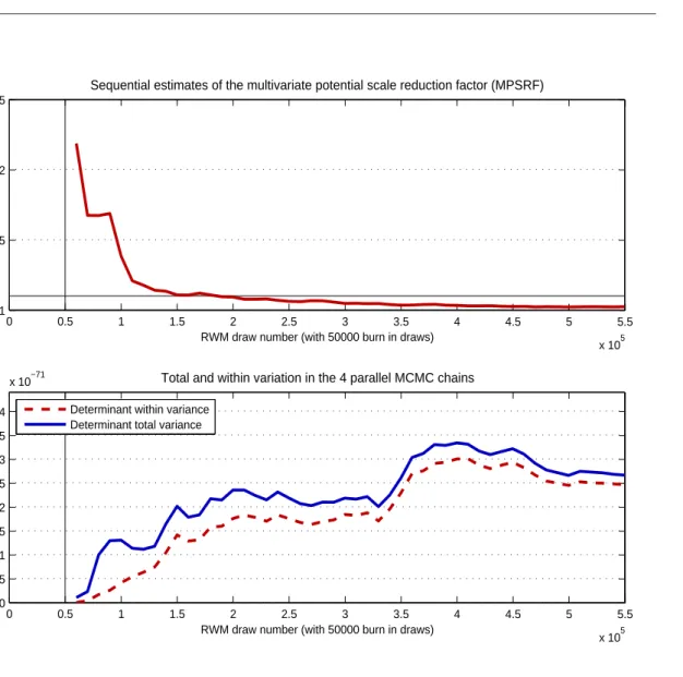
As the posterior distribution cannot be determined analytically, we adopt a Monte-Carlo Markov-Chain (MCMC) sampling algorithm to simulate the distribution of the parameter
28
For details on the derivation of the log-linear version of the NAWM, see Appendix A.
29
For all computations, we use YADA, a Matlab program for Bayesian estimation and evaluation of DSGE models (cf. Warne, 2008).
vector θ.30 The resulting posterior distribution is typically characterised by measures of central location, such as the mode or the mean, measures of dispersion, such as the standard deviation, or selected percentiles.
As discussed in Geweke (1999), Bayesian inference also provides a framework for com-paring alternative, not necessarily nested, and potentially misspecified models on the basis of their marginal likelihood. For a given modelm the latter is computed by integrating out the parameter vector θ,
L(YT|m) =
Z
θ∈Θ
L(YT|θ, m)p(θ|m)dθ.
Thus, the marginal likelihood gives an indication of the overall likelihood of the observed data conditional on a model.
3.2 Data and Shocks
3.2.1 Data
In estimating the NAWM, we use times series for 18 macroeconomic variables which feature prominently in the ECB/Eurosystem staff projections:
• real GDP (Y) • total employment (E)
• private consumption (C) • compensation per head (W)
• total investment (I) • nominal interest rate (R)
• government consumption (G) • nominal effective exchange rate (S)
• extra-euro area exports (X) • foreign demand (Yd,∗)†
• extra-euro area imports (IM) • foreign prices (P∗
Y)†
• GDP deflator (PY) • foreign interest rate (R∗)†
• consumption deflator (PC) • competitors’ export prices (PXc,∗)† • extra-euro area import deflator (PIM) • oil prices (PO)†
All time series are taken from an updated version of the AWM database (see Fagan, Henry and Mestre, 2001), except for the time series of extra-euro area trade data the construction of which is detailed in Dieppe and Warmedinger (2007). The sample period
30
More specifically, we rely on the Random-Walk Metropolis (RWM) algorithm to obtain a large number of random draws from the posterior distribution ofθ. The mode and a modified Hessian of the posterior distribution, the latter evaluated at the mode, are used to determine the initial proposal density for the RWM algorithm. The posterior mode and the Hessian matrix are computed by standard numerical optimisation routines, namely Christopher Sims’ optimiser csminwel.