Analysis
Kashif Yousuf
Submitted in partial fulfillment of the requirements for the degree
of Doctor of Philosophy
in the Graduate School of Arts and Sciences
COLUMBIA UNIVERSITY
Kashif Yousuf All Rights Reserved
Essays in High Dimensional Time Series Analysis Kashif Yousuf
Due to the rapid improvements in the information technology, high dimensional
time series datasets are frequently encountered in a variety of fields such as
macroe-conomics, finance, neuroscience, and meteorology. Some examples in economics and
finance include forecasting low frequency macroeconomic indicators, such as GDP or
inflation rate, or financial asset returns using a large number of macroeconomic and
financial time series and their lags as possible covariates. In these settings, the
num-ber of candidate predictors (pT) can be much larger than the number of samples (T), and accurate estimation and prediction is made possible by relying on some form of
dimension reduction. Given this ubiquity of time series data, it is surprising that few
works on high dimensional statistics discuss the time series setting, and even fewer
works have developed methods which utilize the unique features of time series data.
This chapter consists of three chapters, and each one is self contained.
The first chapter deals with high dimensional predictive regressions which are
widely used in economics and finance. However, the theory and methodology is mainly
developed assuming that the model is stationary with time invariant parameters.
This is at odds with the prevalent evidence for parameter instability in economic
time series. To remedy this, we present two L2 boosting algorithms for estimating
high dimensional models in which the coefficients are modeled as functions evolving
smoothly over time and the predictors are locally stationary. The first method uses
componentwise local constant estimators as base learner, while the second relies on
componentwise local linear estimators. We establish consistency of both methods,
forecasting with many potential predictors, we find that the benefits to modeling
time variation are substantial and are present across a wide range of economic series.
Furthermore, these benefits increase with the forecast horizon and with the length of
the time series available for estimation. This chapter is jointly written with Serena
Ng.
The second chapter deals with high dimensional non-linear time series models, and
deals with the topic of variable screening/targeting predictors. Rather than assume a
specific parametric model a priori, this chapter introduces several model free screening
methods based on the partial distance correlation and developed specifically to deal
with time dependent data. Methods are developed both for univariate models, such
as nonlinear autoregressive models with exogenous predictors (NARX), and
multi-variate models such as linear or nonlinear VAR models. Sure screening properties are
proved for our methods, which depend on the moment conditions, and the strength
of dependence in the response and covariate processes, amongst other factors. Finite
sample performance of our methods is shown through extensive simulation studies,
and we show the effectiveness of our algorithms at forecasting US market returns.
This chapter is jointly written with Yang Feng.
The third chapter deals with variable selection for high dimensional linear
station-ary time series models. This chapter analyzes the theoretical properties of Sure
In-dependence Screening (SIS), and its two stage combination with the adaptive Lasso,
for high dimensional linear models with dependent and/or heavy tailed covariates
and errors. We also introduce a generalized least squares screening (GLSS)
proce-dure which utilizes the serial correlation present in the data. By utilizing this serial
correlation when estimating our marginal effects, GLSS is shown to outperform SIS
List of Figures iv
List of Tables vi
Chapter 1
Boosting High Dimensional Predictive
Regres-sions with Time Varying Parameters
11.1 Introduction . . . 1
1.2 The Econometric Framework . . . 6
1.3 Boosting High Dimensional TVP Models . . . 10
1.4 Implementation . . . 16
1.5 Asymptotic Theory . . . 19
1.6 Simulations . . . 23
1.6.1 Methods and Forecast Design . . . 24
1.6.2 Results. . . 26
1.7 Application to Macroeconomic Forecasting . . . 28
1.7.1 Methods and Forecast Design . . . 31
1.8 Results . . . 33
1.8.1 Analyzing Performance Over Time . . . 34
1.8.2 Assessing Benefits of Modeling Time Varying Parameters . . . 36
1.9 Conclusion . . . 40
relation with Applications to Financial
Fore-casting
812.1 Introduction . . . 81
2.1.1 Our Contributions . . . 83
2.1.2 Comparisons to Existing Work. . . 86
2.1.3 Organization . . . 86
2.2 Review of Distance Correlation Based Methods . . . 87
2.2.1 Preliminaries . . . 87
2.2.2 Partial DC vs Conditional DC . . . 89
2.3 Screening Algorithms . . . 90
2.3.1 Screening Algorithm I: PDC-SIS. . . 92
2.3.2 Screening Algorithm II: PDC-SIS+ . . . 93
2.3.3 Threshold Selection . . . 95
2.4 Screening for Multivariate Time Series Models . . . 96
2.5 Simulations . . . 99
2.5.1 DGP’s . . . 100
2.5.2 Results. . . 102
2.6 Real Data Application: Forecasting Portfolio Returns . . . 103
2.7 Asymptotic Properties . . . 110
2.7.1 Dependence Measures . . . 110
2.7.2 Asymptotic Properties: PDC-SIS . . . 112
2.7.3 Asymptotic Properties: PDC-SIS+ . . . 117
2.8 Discussion . . . 118
2.9 Appendix A . . . 119
2.9.1 Comparing Partial DC vs Conditional DC . . . 120 ii
2.10.1 Sure Screening Properties for Group PDC-SIS . . . 123
2.10.2 Simulations for group PDC-SIS . . . 124
2.10.3 Real data application: Group PDC-SIS . . . 126
2.11 Appendix C: Proofs of Theorems 3 and 4 . . . 128
2.12 Appendix D: Tables for Section 2.5 . . . 141
Chapter 3
Variable Selection for Linear High Dimensional
Time Series Models
146 3.1 Introduction . . . 1463.2 Preliminaries . . . 152
3.3 SIS with Dependent Observations . . . 154
3.3.1 SIS with dependent, heavy tailed covariates and errors . . . . 155
3.3.2 Ultrahigh Dimensionality under dependence . . . 159
3.4 Generalized Least Squares Screening (GLSS) . . . 162
3.5 Second Stage Selection with Adaptive Lasso . . . 169
3.6 Simulations . . . 174
3.7 Real Data Example: Forecasting Inflation Rate . . . 178
3.8 Discussion . . . 181
3.9 Appendix . . . 182
3.9.1 Proofs of Results . . . 182
3.9.2 Asymptotic Distribution of GLS estimator . . . 195
Bibliography 198
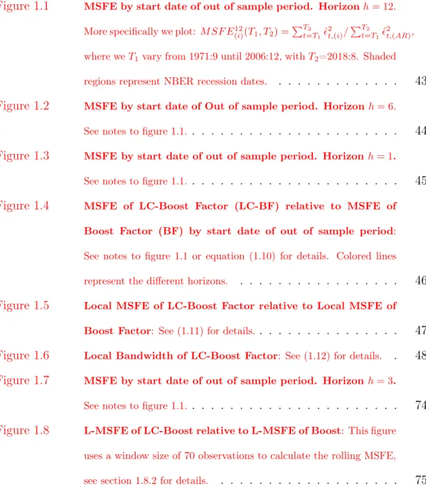
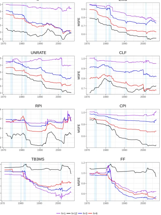
Figure 1.1 MSFE by start date of out of sample period. Horizonh= 12. More specifically we plot: M SF E12
(i)(T1, T2) = PT2 t=T1ˆ 2 t,(i)/ PT2 t=T1ˆ 2 t,(AR),
where weT1vary from 1971:9 until 2006:12, withT2=2018:8. Shaded
regions represent NBER recession dates. . . 43
Figure 1.2 MSFE by start date of Out of sample period. Horizonh= 6. See notes to figure 1.1. . . 44
Figure 1.3 MSFE by start date of out of sample period. Horizonh= 1.
See notes to figure 1.1. . . 45
Figure 1.4 MSFE of LC-Boost Factor (LC-BF) relative to MSFE of
Boost Factor (BF) by start date of out of sample period:
See notes to figure 1.1 or equation (1.10) for details. Colored lines represent the different horizons. . . 46
Figure 1.5 Local MSFE of LC-Boost Factor relative to Local MSFE of Boost Factor: See (1.11) for details. . . 47
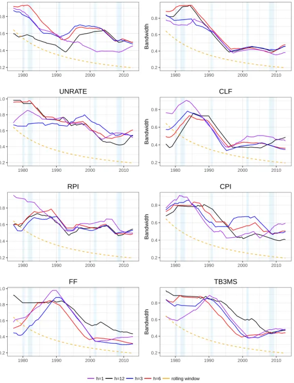
Figure 1.6 Local Bandwidth of LC-Boost Factor: See (1.12) for details. . 48
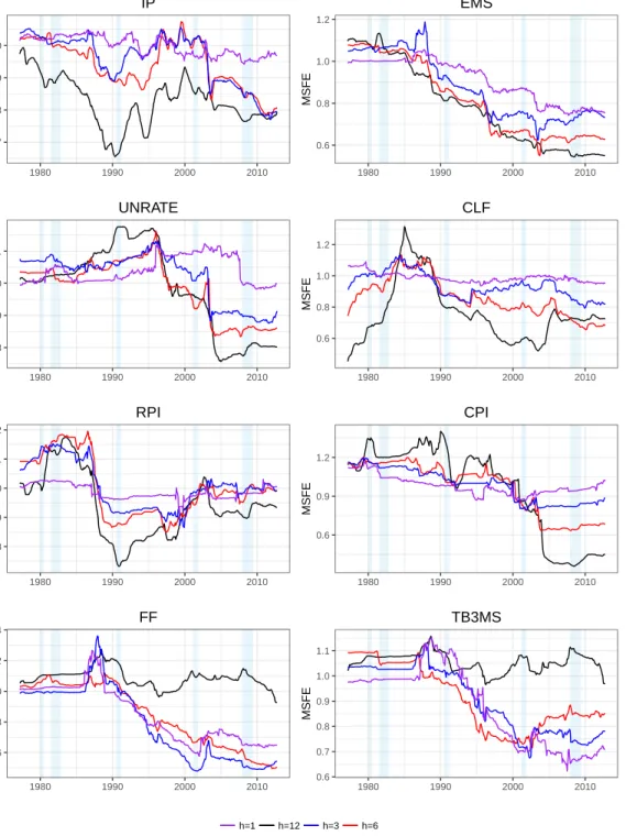
Figure 1.7 MSFE by start date of out of sample period. Horizonh= 3.
See notes to figure 1.1. . . 74
Figure 1.8 L-MSFE of LC-Boost relative to L-MSFE of Boost: This figure uses a window size of 70 observations to calculate the rolling MSFE, see section 1.8.2 for details. . . 75
tor: This figure uses a window size of 70 observations to calculate the rolling MSFE, see section 1.8.2 for details. . . 76
Figure 1.10 L-MSFE of Boost Factor using 10 year rolling window
rela-tive to L-MSFE of LC-Boost Factor: This figure uses a window
size of 70 observations to calculate the rolling MSFE, see section 1.8.2 for details. . . 77
Figure 1.11 L-MSFE of TV-DI relative to L-MSFE of LC-Boost Factor: This figure uses a window size of 90 observations to calculate the rolling MSFE, see section 1.8.2 for details. . . 78
Figure 1.12 L-MSFE of LC-Boost Factor relative to L-MSFE of LL-Boost Factor: We use a window size of 70observations, see notes to figure 1.5 for details. Colored lines represent the different horizons. . . 79
Figure 2.1 R2OOS by Sample Split Date. We select each date between 1960:1-1995:1 as our sample split point and plot the corresponding R2
OOS. We omit the values for GLSS-FAAR and PDC+-FAAR due to having very close results to SIS-FAAR and PDC-FAAR respectively. We used 100 FF portfolios and their lags as possible predictors. . . 109
Figure 3.1 GLS vs OLS error comparison for values of ρ between .5 and .95 incrementing by .05. Absolute error averaged over 200 replications. . . 163
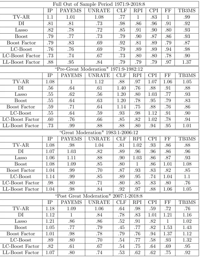
Table 1.1 Relative MSFE, Gaussian Innovations . . . 28
Table 1.2 Relative MSFEh= 12 . . . 42
Table 1.3 Relative MSFEh= 6 . . . 71
Table 1.4 Relative MSFEh= 3 . . . 72
Table 1.5 Relative MSFEh= 1 . . . 73
Table 1.6 DGP 1-14:Relative MSFE, t5 Innovations . . . 80
Table 2.1 Median Minimum Model Size . . . 90
Table 2.2 Median Minimum Model Size . . . 104
Table 2.3 R2 OOS(%) . . . 108
Table 2.4 R2 OOS(%), Excluding AR(1) Term . . . 108
Table 2.5 R2 OOS(%), Size Sorted Portfolios . . . 110
Table 2.6 R2 OOS(%), Size Sorted Portfolios . . . 110
Table 2.7 Partial DC (PDC) vs Conditional DC (CDC): Empirical Power . . . 123
Table 2.8 Model 6 . . . 126
Table 2.9 Group Selection . . . 127
Table 2.10 Model 1 . . . 142
Table 2.11 Model 2 . . . 143
Table 2.12 Model 3 . . . 144
Table 3.1 Case 1 . . . 175
Table 3.2 Case 2: Scenario A . . . 176
Table 3.3 Case 2: Scenario B . . . 177
Table 3.4 Case 3: Scenario A . . . 178
Table 3.5 Case 3: Scenario B . . . 178
Table 3.6 Inflation Forecasts: 12 month horizon . . . 181
I would like to thank a number of key individuals whose thoughtful guidance and
advising supported the completion of this dissertation. First, I would like to
acknowl-edge the training and feedback provided by my advisor Yang Feng. I would also like
to thank Serena Ng, who has unofficially been a second advisor to me, for all the
in-tellectual support and direction on the application of my work to economic contexts.
Without their patience and guidance this thesis would not have been completed. I
would also like to thank Professors Cindy Rush, Victor De La Pena, and Qingfeng
Liu for agreeing to be a part of my commitee.
This dissertation also benefited from countless colleagues in the Department of
Statistics at Columbia. I would like to thank Florian Stebbegg, Jon Auerbach, Adji
Dieng, Wenda Zhou and others for their friendship and intellectual discussions
mo-tivating some of the completion of this work. I would also like to thank Professor
Arian Maleki for his friendship and academic support. I had the opportunity to
in-teract with many individuals across our department - from administrative staff such
as Dood and Anthony who were able to handle any troubles encountered along the
way, to professors, all of whom played an important role in the growth of my career
and education.
Along the way my support system and many friendships have sustained the energy
which facilitated the completion of this PhD. I would also like to thank my parents
for their support throughout my life. Their positivity and faith in me has helped me
This work could not have been written without their blessings and encouragement.
Chapter 1
Boosting High Dimensional Predictive Regressions with Time
Varying Parameters
1.1
Introduction
Due to the rapid improvements in the information technology, high dimensional
time series datasets are frequently encountered in a variety of fields in economics and
finance (see Fan et al. (2011c); Shapiro (2017) for examples). In these settings, the
number of candidate predictors (pT) is much larger than the number of samples (T), and accurate estimation and prediction is made possible by relying on some form of
dimension reduction. Ng(2013) puts the methods used in high dimension predictive
regressions into two classes: a dense class which assumes that the covariates have a
low rank representation that can be exploited for subsequent modeling, and a sparse
class which assumes that the number of relevant predictors is far smaller than the
number of predictors available. Research within the first class usually assumes a
linear latent factor model which is estimated by principal components or partial least
squares.1 The second class treats the problem as one of variable selection in high
dimension. Prominent methods in this class include screening, penalized likelihood,
lasso, and boosting methods.
This paper contributes to the literature in the second class. A key assumption
made in the vast majority of works on sparse modeling is of a stationary underlying
model with time invariant parameters.2 The assumption is very restrictive in practice,
as empirical evidence of parameter instability and time varying effects have been well
documented in macroeconomics.3 Parameter instability can be driven by structural
changes in technological advancements, government or monetary policy changes, and
preference shifts at the individual level (Chen and Hong, 2012). Ignoring these
in-stabilities can lead to large forecasting errors, withClements and Hendry(1996) and
others even arguing that these instabilities are the main source of error for forecasting
models.
Consider a high dimensional linear time varying parameter (TVP) model:
Yt=βtxt−h+t for t= 1, . . . , T, (1.1)
where Yt is the response, xt−h = (X1,t−h, . . . , XpT,t−h) is a pT-dimensional vector of
predictors (withpT >> T),β= (β1,t, . . . , βpT,t)is a vector of time varying parameters,
and t are errors; the precise assumptions on the model will be stated in section 1.3. Given the evidence for parameter instability, the question remains on how to best represent and model this change, especially when dealing with high dimensional
predictors. Parameter instability is most commonly represented in the econometrics
2Examples includeMedeiros and Mendes(2016),Kock and Callot(2015),Han and Tsay(2017),
and Basu and Michailidis (2015) which focus on the Lasso or the adaptive Lasso, and Lutz and Bühlmann(2006) which focuses onL2 boosting for stationary VAR models.
3See (Stock and Watson, 1996; Rossi, 2013; Hamilton, 1989), asset pricing (Goyal and Welch,
2003;Paye and Timmermann, 2006; Rapach et al., 2010; Dangl and Halling, 2012), and exchange rate prediction (Schinasi and Swamy,1989).
literature by random walks or by one or more discrete structural breaks.4 Modeling
variations by random walks can be quite restrictive as it imposes a specific structure
on the evolution of the parameters. Discrete breaks require knowledge of the break
dates, and not all time variations are well characterized by discrete shifts. Technology
and taste shifts are arguably evolving slowly over time. Smooth transition models as
in Terasvirta (1994) are still tightly parameterized. Furthemore, these methods are
mainly designed for a fixed pT. A third approach is to use rolling-window estimation to capture the smooth change in the parameters. As will soon be clear, rolling-window
estimation is a special case of our proposed approach with a particular choice of kernel
and bandwidth.
In this paper, we model these high-dimensional parameters as smooth functions of
time whose functional forms are unknown and are estimated non-parametrically. We
present two L2 boosting algorithms which differ in their choice of base learners; the first uses componentwise local constant estimators as base learners, while the second
relies on componentwise local linear estimators as base learners. We consider the use
of local linear estimators since they have been shown to be a superior estimator
the-oretically, with smaller asymptotic bias at the boundaries of the sample (Cai, 2007).
We establish consistency of both our methods when dealing with high dimensional
locally stationary predictors and errors with only polynomially decaying tails.
Al-though we focus on linear time varying parameter models, L2 boosting methods can easily be adapted to fit more general non-linear models by considering alternative
base learners such as regression trees with varying degrees of depth. This makes
the L2 boosting framework more flexible than the often used `1 penalized likelihood
4The first approach has a long history in macroeconomics, some examples includeCogley and
Sargent(2001);Primiceri(2005);Koop and Korobilis(2013). For the literature on structural breaks, seePerron et al.(2006);Casini and Perron(2018) for surveys.
approaches.
The smooth TVP model considered in this paper has been studied in the
econo-metrics literature for the case when the number of predictors is fixed and assumed
known. Under this assumption,Robinson(1989, 1991) studied the asymptotic
prop-erties of the local constant estimator of the coefficient functions. The theory was
further developed in several directions.5 To our knowledge, there were only two
attempts at modeling sparse high dimensional smooth TVP models, both dealing
with locally stationary sub-Gaussian predictors, and rely on l1 regularization
meth-ods along with kernel smoothing to estimate the coefficient functions. In particular,
Ding et al. (2017) deals with locally stationary sparse VAR processes, and proposes
a hybrid estimator which combines l1 regularization with local constant estimation. Lee et al. (2016) deals with models where the set of non-zero coefficient functions
does not change with over time, and proposes a computationally intensive penalized
local linear estimation method. Our work adds to this line of research by proposing
L2 boosting algorithms for high dimensional smooth TVP models characterized by
(1.1).
Our methods compare favorably to more commonly used alternatives for modeling
time varying parameters such as assuming the coefficients are stochastic and generated
by a random walk, or using a rolling window estimator with a fixed window length.
These models are typically estimated via MCMC, or other computationally intensive
methods, which excludes the use of high dimensional datasets. Rolling window
fore-5 Some examples include: Orbe et al. (2005, 2006) considered shape restricted estimation. Cai
(2007) analyzed the asymptotic properties of the local linear estimator. Inoue et al.(2017) considered the question of optimal bandwidth selection for the local constant estimator when using the uniform kernel. Zhang et al.(2015),Hu et al.(2018), andVogt et al.(2012) allow for non-stationary predic-tors and non-linear time varying functions of these predicpredic-tors. Zhou and Wu (2009);Zhou (2010) considered local linear quantile estimation, Phillips et al.(2017) obtained results for cointegration models, andChen(2015) dealt with models with endogenous predictors.
casts, although they are usually not presented this way, are actually equivalent to
using a local constant estimator using a uniform kernel and a fixed bandwidth. This
choice of fixed bandwidth is arbitrary and can lead to larger forecast errors vs using
the optimal bandwidth (Inoue et al., 2017). Additionally, local constant estimators
have higher asymptotic bias at the boundary of the sample vs local linear estimators.
In contrast, ourL2 boosting algorithms are capable of variable selection and estima-tion simultaneously at a very low computaestima-tional cost even for very high dimensional
data. Also, using non-parametric methods to estimate the time varying coefficient
functions allows our method to perform well even under model misspecifications such
as discrete breaks, stochastic coefficients generated by a random walk, and time
in-variant coefficients; seeGiraitis et al. (2013); Inoue et al. (2017) and our simulations
section for more details.
On the empirical side we include an extensive application to macroeconomic
fore-casting. Although parameter instability has long been established in the econometrics
literature (Stock and Watson, 2003, 2009; Breitung and Eickmeier, 2011), the
ques-tion of whether one can exploit this instability to improve macroeconomic forecasts
is far less clear (see section 1.7 or Rossi (2013) for more details). Some issues which have hindered the utility of modeling time variation are: 1) the bias-variance tradeoff
encountered when using a reduced sample for modeling, 2) misspecification and/or
estimation error incurred when trying to estimate the nature of time variation, and
3) computational constraints restricting the use of high dimensional predictors when
estimating traditional TVP models with stochastic coefficients.
To analyze the effectiveness of modeling time variation with our methods, we use
a panel of 123 monthly series from the FRED-MD database and focus on forecasting 8
major macroeconomic series over a range of forecast horizons. Using an out of sample
our methods are substantial, especially when considering longer forecast horizons,
2) the benefits of using our time varying boosting models vs their time invariant counterparts increases as the length of the available sample increases, and 3) the benefits of modeling time variation appear to be confined to the high dimensional
setting, as we confirm the results in Stock and Watson (1996) that modeling time
variation in AR models offers little to no benefits for the majority of series.
The rest of the paper is organized as follows. Section 1.2 reviews the locally sta-tionary framework, along with the functional dependence measure which will be used
to quantify dependence. We also discuss the assumptions placed on the structure of
the covariate and response processes; these assumptions are very mild, allowing us
to represent a wide variety of stochastic processes which arise in practice. Section
1.3 introduces our boosting algorithms for both local constant or local linear least squares base learners, and studies the asymptotic properties of these procedures. The
asymptotic properties, and the number of predictors allowed depend on the strength
of dependence, and the moment conditions of the underlying processes. Section 1.6
presents results from Monte Carlo simulations, and section1.7 contains our applica-tion to macroeconomic forecasting. Lastly, concluding remarks are in secapplica-tion 1.9.
1.2
The Econometric Framework
We first start with a review of locally stationary processes which were first
in-troduced by Dahlhaus (1996); Dahlhaus et al. (1997) using a time varying spectral
representation. This was expanded in Dahlhaus et al. (2018) to a more general
def-inition which facilitated theoretical results for a large class of non-linear processes;
see Dahlhaus (2012) for a partial survey of the results pertaining to locally
process which can be well approximated by a stationary process locally in time. This
is a convenient framework to model non-stationarity induced by smooth time varying
parameters. Consider the model (1.1), withβt being a vector of unknown determin-istic smooth functions of time, as a consequence Yt in (1.1) is clearly non-stationary. Due to this non-stationarity, letting T → ∞ will not lead to consistent estimates of
βt, since future observations may not contain any information about the probabilistic
structure of the process at the present time t. Therefore, it is common to work in the infill asymptotics framework with rescaled time t/T ∈ [0,1], with βt = β(t/T) (Dahlhaus et al.,1997;Robinson,1989; Cai,2007). Letting T → ∞ now implies that we observe β(t/T) on a finer grid within the same interval, thereby increasing the amount of local information available. Although this setting is not commonly seen in
forecasting time series, a prediction theory is still possible. For example, we can view
our data as having been observed fort = 1, . . . , T /2(i.e. on the interval [0,1/2]), and we are forecasting the next few observations (see Dahlhaus et al. (1997); Dahlhaus
(1996)).
For a formal description of locally stationary processes we use the definition and
assumptions stated in Dahlhaus et al.(2018) and Richter and Dahlhaus (2018):
Definition 1.2.1. Let q > 0, and ||W||q = (E|W|q)1/q. Let Yt,T, t = 1, . . . , T be a triangular array of stochastic processes. For each u∈[0,1], let Y˜t(u)be a stationary and ergodic process satisfying:
1. Dq = max{supu∈[0,1]||Y˜t(u)||q,supT∈N supt=1,...,T||Yt,T||q}<∞
2. There exists CB >0 such that uniformly in t= 1, . . . , T and u, v ∈[0,1]:
From the second assumption we obtain: ||Yt,T−Y˜t(u)||q ≤O(|t/T−u|+T−1), thus for rescaled time points t/T near u, the process Yt,T can be approximated by a sta-tionary process Y˜t(u) with asymptotically negligible error. Consider the model used in Robinson (1989); Cai (2007): Yt,T = β(t/T)Xt+t, where Xt, t are stationary processes, and β(·) is a lipschitz continuous function. Under these conditions Yt,T is a locally stationary process, with stationary approximation: Y˜t(u) =β(u)Xt+t. A slightly more complicated example is a tvAR(1) process: Yt,T =α(t/T)Yt−1,T +t = P∞
j=0[ Qj−1
k=1α( t−k
T )]t−j. Intuitively one can see that if we assume α(·) is lipschitz continuous then the process is locally stationary with stationary approximation:
˜
Yt(u) = α(u) ˜Yt−1(u) + t, and ||Yt,T −Y˜t(u)||q ≤ O(|t/T − u|+ T−1).6 The sta-tionary approximation is the key to estimation and formulating an asymptotic theory
when dealing with locally stationary processes. Estimation of parameters such as
α(u)and local covariances is carried out by assuming, for each rescaled time point u, that the process is essentially stationary on a small window aroundu. We then carry out estimation via stationary methods using observations within this window.7
In order to establish asymptotic properties of our L2 boosting procedures, we
rely on the functional dependence measure used in the context of locally stationary
processes inDahlhaus et al. (2018);Richter and Dahlhaus (2018). We first introduce
the following notation: Let{et}t∈Z be a sequence of iid random variables, and letFt= (et, et−1, . . .), Ft∗ = (et, et−1, . . . , e∗0, e−1, . . .) with e∗0, et, t∈ Z being iid. Additionally,
let Ht = (ηt,ηt−1, . . .), H∗t = (ηt,ηt−1, . . . ,η0∗,η−1, . . .) with η0∗,ηt, t ∈ Z being iid
random vectors. Throughout this paper, we assume the following structure for the
6Under appropriate conditions, more general non-linear time varying processes which satisfy
the recursion: Yt,T = Gt(Yt−1,T, . . . , Yt−p,T,max(t/T,0)), fort ≤ T, can be shown to be locally stationary (Dahlhaus et al., 2018). Examples of such processes include time varying ARMA, time varying GARCH, time varying VAR, and time varying random coefficient processes.
7We note that assuming approximate stationarity on a small window is essentially the justification
stationary approximation for univariate processes (such as the response and error
processes), and multivariate processes (such as the covariate process) respectively:
˜
Yt(u) =g(u,Ft) and x˜t(u) =h(u,Ht) = (h1(u,Ht), . . . , hpT(u,Ht)), (1.3)
where g(·,·), and h(·,·) are real valued measurable functions. These representa-tions allow us to define the functional dependence measure as: δqY˜(u)(t) = ||Y˜t(u)− g(u,F∗
t)||q, and δ ˜ Xj(u)
q (t) = ||X˜j,t(u)− hj(u,H∗t)||q. Additionally, we assume short range dependence of the form:
∆Y0˜,q = ∞ X k=0 sup u∈[0,1] δqY˜(u)(k)≤ ∞, and Φx0˜,q = max j≤pT ∞ X k=0 sup u∈[0,1] δX˜j(u) q (k)≤ ∞, (1.4) for some q >2to be specified in the next section.
We place assumptions on the stationary approximation rather than directly on
the process itself. This leads to results using weaker assumptions, and to more
in-terpretable dependence measures. For an intuitive explanation of this measure, we
consider the stationary approximation at time u0 (Y˜t(u0)) and we obtain δ ˜ Y(u0) q (k) = ||Y˜k(u0)−g(u0,Fk∗)||q. We can viewδ ˜ Y(u0)
q (k)as measuring the dependence ofY˜k(u0)
on the innovation0, which for weakly dependent processes decreases suitably quickly
as k → ∞. For a concrete example, consider a stationary AR(1) process Y˜t(u0) = P∞
j=0a(u0)jet−j with ei iid, then δ ˜ Y(u0) q (k) = |a(u0)k|||e0−e∗0||q, and ∆ ˜ Y(u0) 0,q =||e0 − e∗0||qP ∞ k=0|a(u0)
k|. Now in the locally stationary setting, we take the supremum over the rescaled time interval to account for the non-stationarity of the processes, thereby
obtaining∆Y˜
0,q =||e0−e∗0||qsupu∈[0,1] P∞
k=0|a(u)
k|. A very wide variety of locally sta-tionary processes encountered in practice including time varying linear processes,
processes have stationary approximations which satisfy (1.4), and have geometrically decaying functional dependence measures (see Dahlhaus et al. (2018)).
1.3
Boosting High Dimensional TVP Models
Ever since the introduction of AdaBoost in the 1990’s (Freund and Schapire,
1997), boosting algorithms have been one of the most successful and widely utilized
machine learning methods (Friedman et al., 2001). AdaBoost, which was developed
for classification, consisted of iteratively fitting a series of weak classifiers or learners
onto reweighted data and taking a weighted average of the predictions from each of
these simple models. The success of AdaBoost was originally thought to originate
from averaging many weak classifiers and from a reweighting scheme which placed
large weights on heavily misclassified observations. Later work by Friedman (2001),
and Friedman et al. (2000) established AdaBoost as a gradient descent algorithm in
function space using an exponential loss function. This functional gradient descent
view connected boosting to the common optimization view of statistical inference,
and led to extensions of boosting beyond the realm of classification. Friedman (2001)
proposed several new boosting algorithms using alternative base learners and loss
functions including squared error loss, leading to L2 boosting. Additionally, Efron et al.(2004) andFriedman et al. (2001), made connections for linear models between
L2 boosting and common statistical procedures such as the Lasso and forward
stage-wise regression.8 9 These insights shed light on L
2 boosting as a method which
performs variable selection and shrinkage leading to sparse models. For an excellent
8For theoretical connections one can consult Chapter 16.2 of Friedman et al.(2001), and
addi-tional works such asHastie et al.(2007);Rosset et al.(2004)
9Empirical comparisons between boosting with linear least squares learners and the lasso have
shown close performance with boosting performing slightly better in the case of high correlated predictorsHastie et al.(2007);Hepp et al.(2016).
survey of the statistical view of boosting and results pertaining to several common
boosting algorithms, one can consult Buhlmann and Hothorn(2007). 10
We are interested in estimating the following model:
Yt,T =β0(t/T)xt−h,T +t,T for t= 1, . . . , T, (1.5)
whereYt,T is the response, xt−h,T = (X1,t−h,T, . . . , XpT,t−h,T)
0 is ap
T-dimensional vec-tor of locally stationary predicvec-tors (withpT >> T),β0(t/T) = (β1(t/T), . . . , βpT(t/T))
is a vector of unknown functions of time defined on the grid[0,1], which becomes finer asT → ∞, andt,T denotes the locally stationary error process with E(t,Txt−h,T) = 0∀ t, T. We denote the stationary approximation of the response asY˜t(u) = β0(u) ˜xt−h(u)+ ˜
t(u). To simplify notation, we discuss estimation at the boundary point u=T /T = 1. Before we introduce our boosting algorithms, it helps to first introduce the pop-ulation version of componentwiseL2 boosting with linear base learners as applied to
the stationary approximations( ˜YT(u),x˜T−h(u)):
Algorithm: Population level L2 Boosting
1. Set F(0)(u,x˜
T−h(u)) =E( ˜YT(u))
2. For m= 1, . . . , MT, whereMT is some stopping iteration, do: (a) Compute U˜T(m)(u) = ˜YT(u)−F(m−1)(u,x˜T−h(u)). (b) Let Sm =argminj≤pTE( ˜U (m) T (u)−α (m) j (u) ˜Xj,T−h(u))2, where α(jm)(u) =E( ˜Xj,T−h(u) ˜UT(m)(u))/E( ˜Xj,T−h2 (u)).
10Additionally, one can consultBuhlmann (2006) for extensions of boosting to stationary VAR
processes, and Bai and Ng (2009); Ng (2014) for applications to macroeconomic forecasting and recession classification respectively.
(c) Update F(m)(u,x˜
T−h(u)) = F(m−1)(u,x˜T−h(u)) +υ ·α (m)
Sm(u) ˜XSm,T−h(u),
where υ ∈(0,1] is a step length factor. 3. Output F(MT)(u,x˜
T−h(u)) =F(0)(u,x˜T−h(u)) +υPMm=1T α(Smm)(u) ˜XSm,T−h(u)
Although we use linear base learners, we note that our methods can be
ex-tended to a broader class of models by using a more general base learner, such as
gj(u,X˜j,T−h(u)) = E( ˜YT(u)|X˜j,T−h(u)), and estimating using kernel regressions or smoothing splines. For the corresponding sample version of L2 boosting with linear
base learners, it is informative to consider the case of stationary response and
predic-tor processes. In the stationary setting, we can remove the dependence onT and the sample version of our algorithm simplifies to Sˆm = argminj
PT t=1(U (m) t −αˆ (m) j Xt,j)2, whereαˆ(jm)=T−1PT t=1Xj,t−hU (m)
t , assuming E(Xt), E(Yt) = 0, andE(Xt2) = 1. For the case of locally stationary response and predictor processes the situation is more
complicated as the above estimator is inconsistent forα(jm)(u). Intuitively, this incon-sistency arises since observations “far" from rescaled timeucontain little information about the probabilistic structure of the processes at timeu.
To proceed with estimation in the locally stationary setting, ∀m and j ≤ pT, we haveUt,T(m) =αj(m)(t/T)Xj,t−h,T +j,t,T, whereα(jm)(t/T) =E( ˜Xj,t−h(t/T) ˜U (m) T (t/T))/E( ˜X 2 j,t−h(t/T)).11 By local stationarity and assuming appropriate smoothness conditions, we have the following expansion:
αj(m)(t/T) = αj(m)(u) + ˙αj(m)(u)(t/T −u) + ¨αj(m)(c)(t/T −u)2, (1.6)
where α˙(·),α¨(·) denote the first and second derivative respectively of the function, with c between u and t/T. To compute the local constant estimate for αj(m)(u), we
11Recall thatE(X j,t−h,TU (m) t,T )/E(X 2 j,t−h,T) =α (m) j (t/T) +O(T−1)by local stationarity.
ignore the linear term in the Taylor expansion to obtain the following approximation:
Ut,T(m)≈αj(m)(u)Xj,t−h,T+j,t,T fort/T nearu. The local constant estimator forα (m) j (u) is then ˆ α(lc,jm)(u) = PT t=1Kb(t/T −u)Xj,t−h,TU (m) t,T PT t=1Kb(t/T −u)X 2 j,t−h,T , (1.7)
where Kb(x) = b−1K(x/b), is a kernel function and b is the bandwidth. Therefore, ˆ
α(lc,jm)(u) is a weighted least squares estimate, with the weights given by the kernel values. For now, one can think of this estimator as aiming to use information from
observations “near" time T, while discounting information from distant points. A simple example of the local constant estimate is the rolling window estimate: using
the uniform kernelK(x) = 1|x|≤1, with a fixed bandwidth b=b0, we obtain a rolling
window estimate which uses the last b0T observations in our sample.
The local constant estimate is widely used for estimating time varying effects,
however the Taylor expansion of α(jm)(t/T) suggests we can obtain a better ap-proximation by using the linear term in the expansion (1.6). This was analyzed rigorously in Cai (2007), which showed that for boundary points the local linear
estimator is theoretically superior to the local constant estimator. Using the
ex-pansion (1.6), we obtain: Ut,T(m) ≈ αj(m)(u)Xj,t−h,T + ˙α (m)
j (u)Xj,t−h,T(t/T −u) +j,t,T, for t/T near u. Let Zj,t−h,Tθ
(m)
j (u) where Zj,t−h,T = (Xj,t−h,T, Xj,t−h,T(t/T −u)),
θ(jm)(u) = (α(jm)(u),α˙(jm)(u))0. The local linear estimate is obtained by minimizing a weighted least squares criterion:
ˆ θj(m)(u) = ( ˆα(ll,jm)(u),αˆ˙(ll,jm)(u)) =argminθ(m) j (u) T X t=1 Kb(t/T −u)(U (m) t,T −Zt−h,Tθ (m) j (u)) 2 (1.8)
Using these estimators we can formulate ourL2 boosting algorithm for (1.5) using
local constant, and local linear estimators as base learners. We first start with our
first algorithm which uses local constant estimators:
Algorithm 1: Local Constant L2 Boosting (LC-Boost)
1. Set Fˆlc(0)(u,xt,T) = T−1 PT
i=h+1Kb(i/T −u)Yi,T, fort = 1, . . . , T −h 2. For m= 1, . . . , MT, whereMT is some stopping iteration, do:
(a) Compute the residualsUˆi,T(m) =Yi,T−Fˆ( m−1) lc (u,xi−h,T)fori=h+ 1, . . . , T. (b) Let Sˆm =argminj≤pT PT i=h+1Kb(i/T −u)( ˆU (m) i,T −αˆ (m) lc,j(u)Xj,i−h,T)2
(c) Update Fˆlc(m)(u,xi−h,T) = ˆFlc(m−1)(u,xi−h,T) +υαˆlc,S(m)m(u)XSm,i−h,T, where
υ ∈(0,1]is a step length factor. 3. Output Fˆ(MT) lc (u,xT−h,T) = ˆFlc(0)(u,xt,T) +υ PMT m=1αˆ (m) lc,Sm(u)XSm,T−h,T
Letzt,T = (xt,T,xt,T(t/T−u)), our boosting algorithm using local linear estimates as base learners is:
Algorithm 2: Local Linear L2 Boosting (LL-Boost)
1. Set Fˆll(0)(u,xi−h,T) = T−1PTi=h+1Kb(i/T −u)Yi,T, fori=h+ 1, . . . , T 2. For m= 1, . . . , MT, whereMT is some stopping iteration, do:
(a) Compute the residuals Uˆi,T(m) =Yi,T −Fˆ (m−1) ll (xi−h,T)for i=h+ 1, . . . , T. (b) Let Sˆm =argminj≤pT PT i=1Kb(i/T −u)( ˆU (m) i,T −Zj,i−h,Tθˆ (m) j (u))2.
(c) Update Fˆll(m)(u,xi−h,T) = ˆF (m−1)
ll (u,zi−h,T) +υ ·ZSm,i−h,Tθˆ
(m)
Sm(u), where
υ ∈(0,1]is a step length factor. 3. Output Fˆ(MT)
ll (u,xT−h,T) = ˆFll(0)(u,xi−h,T) +υPMm=1T ZSm,T−h,Tθˆ
(m) Sm(u)
We see that boosting is a stagewise estimation procedure, where at each stage
only one learner is updated and the previously selected terms are unchanged. This
stagewise fitting procedure induces regularization through limiting the number of
steps (MT), and the step length factor (υ). We usually fix the the step-length factor (υ) to a low number such as υ =.1, making the stopping iteration (MT) akin to the regularization parameter of the Lasso.12 In light of this, boosting can be thought of
as a close relative of the lasso, with the advantage of being able to approximate the`1
penalized solution in situations where it is impossible or computationally burdensome
to compute the Lasso solution (Friedman et al., 2004).
By viewing boosting as a general regularized function estimation procedure, we
can formulate a generic local constant boosting procedure which can be easily be
computed for a wide variety of base learners and (almost everywhere) differentiable
loss functions (L(·,·)).
Algorithm 3: Generic Local Constant Boosting
1. SetFˆG(0)(u,xt,T) = argmincT −1PT
i=h+1Kb(i/T−u)L(Yi,T, c), fort= 1, . . . , T−h
2. For m= 1, . . . , MT, whereMT is some stopping iteration, do: (a) Compute the pointwise negative gradient:
Ui,T(m) = dFd L(Yi,T, F) F= ˆFG(m−1)(u,xi−h,T) evaluated at i=h+ 1, . . . , T.
12Given that each predictor can be selected multiple times, especially for low values of υ, the
number of predictors in the estimated model is ≤ MT, and all predictors which have not been
(b) Let Sˆm =argminj≤pT PT i=h+1Kb(i/T −u)( ˆU (m) i,T −bg (m) j (u, Xj,i−h,T))2 (c) Update FˆG(m)(u,xi−h,T) = ˆF( m−1) G (u,xi−h,T) + υbg (m) Sm(u, XSm,i−h,T), where
υ ∈(0,1]is a step length factor. 3. Output Fˆ(MT) G (u,xT−h,T) = ˆF (0) G (u,xt,T) +υPMm=1T bg (m) Sm(u, XSm,T−h,T)
The algorithm can be modified to allow gj(u,·) to be a function of several variables e.g. a predictor along with a number of its lags.
1.4
Implementation
Implementation of these algorithms is very simple and can be carried out using
ex-isting software packages. We first discuss the choice of the kernel functionK(·), band-width (b), stopping iteration (MT), and step length factor (υ). We set υ =.1, which is the default choice in statistical software packages and applied work (Buhlmann
and Hothorn,2007;Friedman,2001;Hofner et al.,2014). In non-parametric statistics
and machine learning the most commonly used kernels are the Gaussian Kernel and
the Epanechnikov kernelK(u) =.75(1−u2)1
|u|≤1, while in econometrics the uniform
kernel 1|u|≤1 is more widely used. Both the uniform kernel and the Epanechnikov
Kernel use a subset of the sample, with the Epanechnikov kernel also downweighting
more distant observations within this subset. The Gaussian kernel does not truncate
the sample, instead it smoothly downweights more distant observations. It has a
much smoother downweighting scheme than the Epanechnikov kernel, which can be
beneficial in many applications.13 In general however, the choice of a kernel does not
have much impact on the performance, as opposed to the selection of the bandwidth
parameter which is crucial.
13We decide to use the uniform kernel in our applications due to its close connections with the
We first discuss bandwidth selection for an out of sample forecasting exercise.
To help with exposition, we use a concrete example: assume we have monthly data
ranging from 1960:1 to 2018:8, giving us about ∼ 700 observations. We begin our forecasts on 1970:1 and move forward utilizing an expanding window framework. We
use one-sided kernels to avoid looking into the future. We choose our bandwidth
parameter using a cross validation approach. We first form a grid of values B = (b1, . . . , bn) from which to select the bandwidth parameter. For each forecast, our cross validation procedure uses the last ω (where ω is chosen by the researcher) observations of our sample for an out of sample forecasting exercise. We then choose
the bandwidth which minimizes the MSFE over this sub-sample. Therefore, the
selected bandwidth is:
b∗T 0 =argminbi∈Bω −1 T0−h X τ=T0−ω (Yτ,T −Fˆ (MT) τ,bi (τ /T,xτ−h,T)) 2, whereFˆ(MT)
τ,bi (τ /T,xτ−h,T)refers to the LC-Boost or LL-Boost estimate ofxτ−h,Tβ(τ /T)
using only observations until timeτ, and the bandwidthbi. For our first out of sam-ple forecast we setT0 = 120, which is the length of the sample available at the time,
and for each additional forecast we increment T0 by 1 until we reach the end of the
sample. In the special case of using LC-Boost with a one sided uniform kernel, we
are selecting the optimal window size at each time point, via cross validation, for a
rolling window forecast. With the bandwidths representing the fraction of the sample
we are using for estimation.
For in-sample estimation problems, two sided kernels are used in our algorithms
The procedure is as follows: b∗T 0 =argminbi∈BT −1 T X τ=h (Yτ,T −Fˆ (MT) lc,−τ,bi(τ /T,xτ−h,T)) 2K bi(τ /T −T0/T), where Fˆ(MT)
lc,−τ,bi(τ /T,xτ−h,T) refers to the estimate of xτ−hβ(τ /T), which uses all
ob-servations except(Yτ,T,xτ−h,T). The kernel in the above equation discounts errors far away from the time point t0 when selecting the optimal bandwidth. This procedure
gives us a bandwidth for each time point in the sample, and if one wants a single
bandwidth for all time points, the kernel can be removed.
To select the stopping iteration MT, we specify an upper bound for the number of iterationsMupp (we set Mupp = 100), where MT ≤Mupp. The stopping iteration is then selected using the corrected AIC (AICc) statistic given in Buhlmann(2006):
MT =argminm≤MuppAICc(m),
whereAICc(m)is the AIC of the model using m iterations.14
Our methods can be computed extremely quickly using the existing R package
mboost. Our base learners are univariate or bivariate weighted least squares esti-mates which can be implemented through existing functions in the package once we
specify the kernel values as weights. We can also implement the generic local
con-stant boosting algorithm for wide a variety of base learners and loss functions such
as absolute loss, Huber loss and quantile loss.15 As an example, to obtain quantiles
14Alternatively, we can jointly select M
T and the bandwidth b∗T0 by forming a two dimensional grid and selecting the optimal combination using the cross validation procedure described earlier. We decide to use theAICcstatistic in this work. We note that when dealing with very large sample
sizes and/or more complicated base learners which are a function of more than one variable, using cross validation to selectMT, using a moderately sized grid, can often be quicker since calculation
of the corrected AIC requires computing the trace of the Hat matrix.
for our forecasts, we specify the quantile loss for a given quantile16, and compute
the optimal bandwidth for our base learners by using the cross validation procedure
mentioned above. A density forecast can be obtained from these estimated quantiles
by using the procedure outlined in?.
1.5
Asymptotic Theory
In order to prove our asymptotic results, we need the following assumptions:
Condition 1.5.1. Assume supu∈[0,1]|β(u)|1 <∞
Condition 1.5.2. Assume the error and the covariate processes are locally stationary and have representations given in (1.3). Additionally, we assume the following decay rates Φx m,r = O(m −αx),∆ m,q = O(m −α), for some α x, α > 0, q > 2, r > 4 and τ = qqr+r >2.
Condition 1.5.3. Let Σ˜x(u) = E( ˜x0t(u) ˜xt(u)) be the covariance matrix function. For u∈ [0,1], assume that β(u),Σx˜(u)∈ C2[0,1], where C2[0,1] denotes the class of
functions defined on[0,1]that are twice differentiable with bounded derivatives.
Condition 1.5.4. The kernel function K(u) is bounded and symmetric, and of bounded variation with compact support. Additionally, the bandwidth (b) satisfies
bT =RT =O(Tψ), where ψ ∈(0,1).
Condition1.5.1requires`1 sparsity of the time varying coefficients, and allows the
active set of predictors to change over time. Our asymptotic results do not require
sparsity in the number of non-zero coefficients (`0 sparsity). Condition1.5.2 assumes
to themboostpackage. It also lists the wide variety of base learners and loss functions supported by the package.
the covariate and error processes are locally stationary, and presents the dependence
and moment conditions on these processes, where higher values of αx, α indicate weaker temporal dependence. We assume our predictor and error processes have at
least r > 4 and q > 2 finite moments respectively. Examples of processes satisfying condition 1.5.2 were given in section1.2.
Given that xt−h can contain lags of Yt,T, an example of a model which satisfies the above conditions is as follows: Let Wt,T = (Yt,T,zt,T), where zt,T represents our exogenous series, andWt,T =P`i=1Ai(t/T)Wt−i,T+ηt. Then the stationary approx-imation is Wft(t/T) =
P`
i=1Ai(t/T)Wft−i(t/T) +ηt, with cumulative functional
de-pendence measure ΦW˜
0,r = supu∈[0,1] P∞
k=0O(λmax(A∗(u))k)(Chen et al., 2013), where
A∗(u) is the companion matrix. We can then define xt−1,T = (Wt−1,T, . . . ,Wt−l,T), andβ(t/T) as the first row of the companion matrixA∗(u). We weaken the assump-tions placed in the worksCai (2007);Robinson(1989); Chen and Hong(2012) which
restricted the predictors and errors to be stationary, thus ruling out models with
lagged dependent variables. Compared to previous works on high dimensional TVP
models, such as Ding et al. (2017); Lee et al. (2016), we use a different dependence
framework, and allow the predictors and errors to have polynomially decaying tails.
Condition 1.5.3 is a sufficient condition to guarantee that the expansion (1.6) ex-ists, i.e: αj(m)(u) ∈ C2[0,1],∀m and j ≤pT. Sufficient conditions needed for smooth-ness of the covariance matrix function were given in Ding et al. (2017) for the case
of locally stationary VAR processes, and one can consult Dahlhaus et al. (2018) for
sufficient conditions for more general processes. Condition 1.5.4 is a standard con-dition and it includes the commonly used Epanechnikov (K(u) = .75(1−u2)1
|u|≤1)
effective sample sizeRT. Let aT = " R−τT +τ κ+1+pTR −r/2+rκ+1 T +pT exp −R1T−2κ + exp −R1T−2κ #
The following two theorems presents the consistency of LC-Boost and LL-Boost.
Theorem 1. Let x∗T−h,T denote a new predictor variable, independent of and with the same distribution as xT−h,T. Let κ∈ (0,1/2) be such that κ < ψ−1−1, Suppose that conditions 1.5.1, 1.5.2, 1.5.3, and 1.5.4 hold. Then
a. on a set with probability at least 1−O(pTaT), our LC-Boost estimateFˆ (MT)
lc (·,·) satisfies: E(|Fˆ(MT)
lc (u,x ∗
uT−h,T)−β0(u)xuT−h,T∗ |2) = op(1) (T → ∞) for some sequence MT → ∞ sufficiently slowly,
b. on a set with probability at least 1−O(pTaT), our LL-Boost estimate Fˆll(MT)(·,·) satisfies E(|Fˆ(MT)
ll (u,x ∗
uT−h,T)−β 0(u)x∗
uT−h,T|2) = op(1) (T → ∞) for some sequence MT → ∞ sufficiently slowly,
This is an extension of theorem 1 in Buhlmann (2006) to the locally stationary
time series setting with local constant or local linear base learners. From the above
theorems, we see the range of pT depends primarily on the moment conditions, the effective sample size RT, and κ. For example, if we assume only finite polynomial moments with r=q,α ≥1/2−2/r then, pT =o(R
r/4−rκ/4−1/2
T )for our estimates to
be consistent. If we assume, subgaussian or subexponential predictors for example
we have pT = o(Tφ) for arbitrary φ > 0. This is the same range Buhlmann (2006) obtained for iid sub-Gaussian predictors and errors. Given the O(T−1) encountered when approximating a locally stationary process by a stationary distribution, we are
unable to extend the theory to the ultra-high dimensional setting i.epT =o(exp(nc)) for c <1.
We also provide results for the stationary time series with time invariant
pa-rameters. In this setting, we use the linear least squares base learner and use the
entire sample for estimation. For the case of only a finite number of moments, the
results in theorem 1 easily carry over to the stationary time invariant setting (i.e
β(t/T) = β ∀t, T), by letting RT = T, and computing the relevant functional de-pendence measures. However, we can obtain a larger range for pT, if we assume a stronger moment condition such as:
Condition 1.5.5. Assume the response and the covariate processes are stationary and have representations given in (1.3). Additionally, assumeυx = supq≥2q
−α˜xΦx
0,q <
∞and υ = supq≥2q −α˜∆
0,q <∞, for someα˜x,α˜ ≥0.
Condition 1.5.5 strengthens the moment condition 1.5.2, and requires that all moments of the covariate and response processes are finite. To illustrate the role of
the constants α˜x and α˜, consider the example where t = P∞
j=0ajet−j with ei iid, and P∞
j=0|aj|< ∞. Then ∆0,q =||e0 −e∗0||q P∞
j=0|aj|. Now if we assume e0 is
sub-Gaussian, then α˜ = 1/2, since ||e0||q =O(
√
q), and if ei is sub-exponential, we have ˜
α = 1.
The following corollary states the corresponding results for the stationary time
series setting. We defineψ˜= 1+2 ˜α2
x+2 ˜α,ϕ˜= 2 1+4 ˜αx, and let bT = " exp −T 1/2−κ υxυ ψ˜ +pT exp −T 1/2−κ υ2 x ϕ˜# , and letFˆ(MT)(x
t)denote our L2 boosting estimate forYt, we then have:
Corollary 2.Letκ∈(0,1/2), andx∗T−h denote a new predictor variable, independent of and with the same distribution asxT−h. Suppose conditions1.5.1, 1.5.4, and1.5.5 hold. Then on a set with probability at least1−O(pTbT), we have that ourL2 Boosting
estimate Fˆ(MT)(·) satisfies:
E(|Fˆ(MT)(x∗
T−h)−βx ∗
T−h|2) =op(1) (T → ∞).
We see that in the stationary setting our theorems improve upon previous results
by providing a more detailed and larger range for pT. For example, assuming sub-Gaussian predictors and errors we obtainpT =o(exp(T
1−2κ
3 )), andpT =o(exp(T 1−2κ
5 ))
for subexponential predictors and errors. As a comparisonBuhlmann(2006) obtained
pT = o(Tφ), for arbitrary φ > 0, when applying L2 boosting for stationary
sub-Gaussian time series.
1.6
Simulations
In this section, we evaluate the forecasting performance of our algorithms in a
finite sample setting. LetYt,T denote our response, and let
xt−1,T = (Yt−1,T, . . . , Yt−3,T,zt−1,T, . . . ,zt−3,T) represent our potential set of predic-tors, wherezt−1,T ∈ RdT represents ourdT exogenous series at timet. We fixT = 200, and dT = 100, giving us pT = 303 potential predictors. We consider 14 DGPs and our general model is, for t= 1, . . . T,
Yt,T = ρYt−1,T + 4 X j=1 (b+βj(t/T))zj,t−1,T +t zt,T = A(t/T)zt−1,T +ηt
and it is assumed thatρ=.6,b = 0.5. For DGPs 1-12 we letA(t/T) = {.4|i−j|+1} i,j≤dT,
and for DGPs 13 and 14 we let A(t/T) = (1−t/T)A1 + (t/T)A2, where the
ma-trices A1 = {.2|i−j|+1}i,j≤dT, A2 = {.4
|i−j|+1}
exp(−γ(t/T −c))−1, time variation in the coefficients is modeled as follows:
DGP Description β1(t/T) β2(t/T) β3(t/T) β4(t/T) zt,T
1 constant 0 0 0 0 stationary
2 break in error variance 0 0 0 0 stationary
3 early break,Tb= 50 −1(t > Tb) stationary
4 mid break,Tb= 100 −1(t > Tb) stationary
5 late break,Tb= 150 −1(t > Tb) stationary
6 small random walk ∆βj(t/T)∼N(0,√.5
T) stationary
7 big random walk ∆βj(t/T)∼N(0,√1T) stationary
8 smooth,c=.25 lgt(10,c) lgt(5,c) lgt(20,c) lgt(10,c) stationary 9 smooth,c=.75 lgt(10,c) lgt(5,c) lgt(20,c) lgt(10,c) stationary 10 smooth,c=.90 lgt(10,c) lgt(5,c) lgt(20,c) lgt(10,c) stationary 11 steep −.3(Tt)2 (Tt)2 −.4(Tt) Tt stationary 12 exotic 0 0 3cos(2πt T ) 2 t Tsin(2π t T) stationary
13 smooth,c=.75 lgt(10,c) lgt(5,c) lgt(20,c) lgt(10,c) locally stationary 14 late break,Tb= 150 −1(t > Tb) locally stationary
For all DGPs, we report results when generating the innovations asηt iid
∼ N(0, IdT)
or from a t5(0,3/5∗IdT). For DGP 2, we have a break in the error variance: t =
D(0,1)(t <150) +D(0,2.5)(t≥150), where the distribution D is either a normal or
t5 distribution. For the remaining DGPs t iid
∼ N(0,1)or iid∼t5.
1.6.1
Methods and Forecast Design
We consider the forecasting performance of the following methods:
• LC-Boost, LL-Boost.
• L2 Boosting, with time invariant coefficients estimated on the full sample.
• Rolling window L2 Boosting, Rolling window AR(3) model both with window
lengthT /5.
AR and rolling window AR models are commonly used benchmarks in macroeconomic
forecasting. Models estimated on the full sample assume time invariant parameters,
or more generally assume the time variation is small. Estimation using LC-Boost,
LL-Boost or a rolling window approach involves using a subsample of the data leading to
a bias-variance tradeoff. Due to this tradeoff, methods accounting for time variation
are not guaranteed to outperform their time invariant counterparts in a finite sample
setting.
All boosting models are computed using the R package mboost, and the lasso model is computed using the R packageglmnet. For LC-Boost and LL-Boost, we use the uniform kernel and we estimate the bandwidth via the cross validation procedure
described in section1.4, with ω= 20, andB = [.3, .4, . . . ,1]. The number of steps in all boosting models is determined using AIC with the maximum number of steps set
toMupp = 100. Lastly, the penalty parameter in the Lasso model is estimated using the BIC statistic.
For each simulation, and for all methods, we forecast YT ,T and compute the out of sample forecast error, which is then averaged over 1000 simulations. Specifically,
for a given simulation, let YˆT,T(k) represent the out of sample forecast of YT ,T. We then compute MSFE=10001 P1000k=1( ˆYT ,T(k) −YT,T(k))2, for each method. We report this MSFE relative to the MSFE obtained from L2 boosting model with time invariant
1.6.2
Results
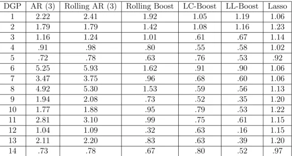
The results for Gaussian innovations are in table1.1. The results fort5 innovations
are contained in the appendix. We first dicuss results for the Gaussian case. DGP
1 and 2 contain time invariant coefficients, with DGP 2 having a structural break in
the variance of the noise. In both these DGPs using the full sample yields the best
estimator. LC-Boost only has a minor error inflation compared to using the whole
sample, whereas LL-Boost does worse than LC-Boost in this setting. The under
per-formance of LL-Boost vs LC-Boost in these settings is likely due to the bias-variance
tradeoff when using local linear vs local constant methods. If the time variation is
non-existent or mild, as is the case here, the additional variance incurred by
estimat-ing more parameters can cancel out any benefit obtained from bias reduction. DGP
3,4,5 all contain a discrete structural break, and we see that both LC-Boost and LL-Boost outperform other methods. When the structural break occurs near the end
of the sample, LL-Boost has large gains over LC-Boost.
DGP 6 has a slowly varying random walk, and we observe that LC-Boost and
LL-Boost perform slightly better than using the full sample. DGP 7 has larger time
variation in the coefficients, and we see that LL-Boost and LC-Boost easily
outper-forms the other methods. DGP 8, 9 and 10 have smooth transition logistic functions,
wherecis the analogous to the breakpoint in a discrete break model, andγ represents smoothness of the transition.17 Out of the three DGPs, time varying methods
per-form best whenc=.75, with the performance deteriorating in the other two cases as the time variation occurs either too close to the forecast date or too far away. DGP
11 and 12 contain coefficient functions which are highly non-linear, and LL-boost
shows very large improvements vs LC-Boost. DGP 13 and 14 show that adding
cally stationary predictors leads to only slight change in the results vs DGP 9 and 5
respectively.
When we have t5 innovations, the results generally follow the conclusions stated
earlier, except the improvements are noticeably smaller in many cases. The presence
of additional noise in the data likely impacts our method in two ways: due to the
additional noise in the data, the bias-variance tradeoff is less favorable to using a
subset of the full sample. Additionally, the noise in the data makes the cross validation
error estimate less reliable, leading to errors in estimating the optimal bandwidth
parameter.18
The results suggest the following conclusions:
1. When the time variation in the coefficients is non-existent or minor, using the
full sample often gives the best performance. The performance of LC-Boost is
only marginally weaker than using the full sample, while the performance of
LL-Boost takes a more significant hit.
2. LL-Boost and LC-Boost forecasts both seem to underperform forecasts using
the full sample when there is a break of in the conditional variance rather than
the conditional mean.
3. Using LL-Boost leads to large improvements in forecasting performance vs
LC-Boost when we have significant time variation in the coefficients. This is
espe-cially true when the time variation occurs closer to the forecast date and/or the
coefficient functions are highly non-linear.
4. Time varying methods are likely to be less useful when we have a low sample
18We also repeated each of the simulations using the Gaussian kernel instead of the uniform kernel.
In general we found very similar performance between the two kernels. For the case oft5innovations
and little to no time variation in the coefficients, we found the Gaussian kernel was more effective for LL-Boost. Given the close similarities between the kernels, we omit the results.
Table 1.1: Relative MSFE, Gaussian Innovations
DGP AR (3) Rolling AR (3) Rolling Boost LC-Boost LL-Boost Lasso
1 2.22 2.41 1.92 1.05 1.19 1.06 2 1.79 1.79 1.42 1.08 1.16 1.23 3 1.16 1.24 1.01 .61 .67 1.14 4 .91 .98 .80 .55 .58 1.02 5 .72 .78 .63 .76 .53 .92 6 5.25 5.93 1.62 .91 .90 1.06 7 3.47 3.75 .96 .68 .60 1.06 8 4.92 5.30 1.53 .59 .56 1.13 9 1.94 2.08 .73 .52 .35 1.20 10 1.77 1.88 .95 .79 .53 1.22 11 2.81 3.10 .99 .75 .61 1.15 12 1.04 1.09 .32 .63 .16 1.15 13 2.11 2.20 .83 .63 .39 1.20 14 .73 .78 .67 .80 .52 .97
size coupled with high noise. Some of the difficulties in this setting may be
overcome by selecting the bandwidth parameter using a larger validation set
along with a finer grid of bandwidth values.
1.7
Application to Macroeconomic Forecasting
As discussed in the introduction, the parameter instability of various
macroeco-nomic series has long been established in the econometrics literature. Some examples
includeStock and Watson (1996, 2009);Breitung and Eickmeier (2011), all of which
find instability in either the univariate relationship of a large number of series or
in the factor loadings of a dynamic factor model of a large panel of macroeconomic
series. Similarly, Stock and Watson (2003) and Rossi and Sekhposyan (2010) have
found evidence of instability in the predictive ability of various series in forecasting
output and inflation. However, the question of whether forecasts can be improved by
far less clear.
Proponents of modeling parameter instability include works such asClements and
Hendry (1996) which argue that ignoring these instabilities are the main sources of
forecast breakdowns. On the other hand, empirical evidence in favor of ignoring
instabilities include Stock and Watson(1996) which had shown there is little benefit
to modeling time variation in a wide range of autoregressive and bivariate forecasts,
and Kim and Swanson (2014); Koop (2013) which showed forecasts estimated by
recursive estimation (using the full sample) performed as well as or better than rolling
window forecasts for a range of models estimated from a large panel of macroeconomic
series. Additionally, a number of works such asPettenuzzo and Timmermann(2017);
Koop and Korobilis (2013); Eickmeier et al. (2015), have estimated TVP models
using Bayesian methods and their results suggest that TVP models offer only minor
improvements in the accuracy of point forecasts when compared to low dimensional
constant parameter models.19 Lastly, on the theoretical side, Bates et al.(2013) has
shown the standard principal components estimator remains consistent even in the
presence of “small" breaks and/or mild time variation in the factor loadings of a
dynamic factor model.
To illustrate the difficulty of exploiting parameter instability, consider a simple
example where there is a single discrete structural break in the forecasting model.
Even if the researcher knew the precise date of the break and decided to use only
post break observations for estimation there is a bias-variance trade off in using less
data for estimation (Pesaran and Timmermann, 2007). Therefore in the presence of
19These works did find TVP models produced larger improvements to density forecasts. We
note that works such as Koop and Korobilis (2012); Groen et al.(2013); Chan et al. (2012) have also estimated TVP models using Bayesian methods and found significant improvements to point forecasts when compared to a low dimensional constant parameter benchmark. However, these works are restricted to forecasting inflation with low dimensional predictors.
small instabilities, such as small breaks or very slowly varying coefficients, using the
entire sample through recursive estimation can be more beneficial than using only a
subset of the data. Due to this bias-variance tradeoff and the uncertainty around the
precise nature of time variation, the majority of works on macroeconomic forecasting
tend to use the full sample available when forecasting. Furthermore, these issues are
more severe when using high dimensional predictors.
Given the above discussion, we use the methods developed in this paper to answer
a number of questions such as:
• Does modeling parameter instability improve macroeconomic forecasts?
• Which models are best able to deal with underlying parameter instability?
• Which variables and forecast horizons benefit most from the use of time varying parameter models?
• During which time periods do time varying methods perform best?
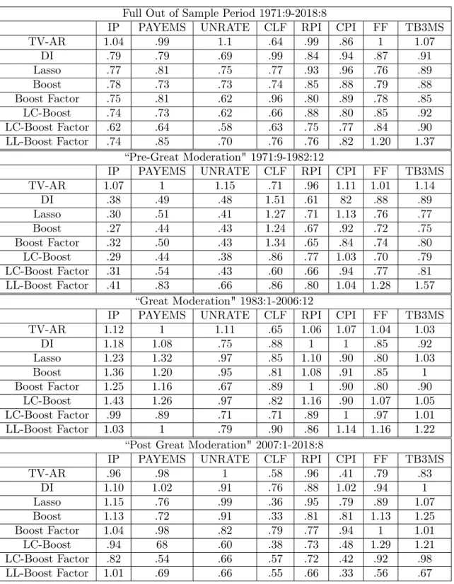
To answer these questions, we use the August 2018 (2018:8) vintage of the
FRED-MD database which contains 128 monthly macroeconomic series collected from a
broad range of categories. SeeMcCracken and Ng (2016) for a more detailed
descrip-tion of each series, as well as transformadescrip-tions needed to achieve approximate stadescrip-tion-
station-arity.20 We remove 5 series which contain large amounts of missing values, leaving
us with 123 monthly macroeconomic series which run from January 1960 to August
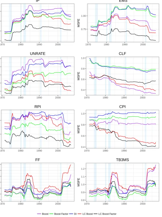
2018. We focus our analysis on 8 major macroeconomic series: Industrial Production
(IP), Total Nonfarm Payroll (PAYEMS), Unemployment Rate (UNRATE), Civilian
Labor Force (CLF), Real Personal Income Excluding Transfer Receipts (RPI),
Con-sumer Price Index (CPI), Effective Fed Funds Rate (FF), and Three Month Treasury
20We depart from the recommended transformations for the housing series (Group 4) which we
Bill (TB3MS). For each series, we compare the out of sample forecasting performance
of several models at theh= 1,3,6,12month forecasting horizons.
1.7.1
Methods and Forecast Design
For all the methods we consider, letYht,T denote ourh-step ahead target variable to be forecast. As an example, for CPI our target variable isYh
t,T = 1200
h log( CP It
CP It−h), and
we define the target similarly for the rest of the series except FEDFUNDS and TB3MS
which are modeled asI(1) in levels (i.e. Yt,Th = 12h(FEDFUNDSt−FEDFUNDSt−h)). Next let zt−h,T denote the rest of our 122 predictor series at time t −h, and let
xt−h= (Yt−h,T, . . . , Yt−h−3,zt−h,T, . . . ,zt−h−3,T)where Yt−h,T =Yt−h,T1 .
For all time varying methods we estimate the bandwidth using the cross validation
procedure detailed in section1.4. For selecting the bandwidth we use a grid of values from .3 to 1 with increments of .025 i.e. B = [.3, .325, . . . . ,1], and we use the last
ω = 60 observations as our validation set.21 Additionally, we estimate all models
under consideration using time invariant methods in order to assess the benefits of
directly modeling time variation. We evaluate the forecasting performance of the
following methods:
Method Parameter Predictors considered AR time invariant (Yt−h,T, . . . , Yt−h−3)
TV-AR local constant (Yt−h,T, . . . , Yt−h−3)
Boost time invariant xt−h
Lasso time invariant xt−h
LC-Boost local constant xt−h
LL-Boost local linear xt−h
LC-Boost-Factor local constant (Yt−h,T, . . . , Yt−h−3,Ft−h,T, . . . ,Ft−h−3,T)
LL-Boost-Factor local linear