Distributed and Parallel
Methods for Structural Convex
Optimization
Jueyou Li
This thesis is submitted in total
fulfilment of the
requirement for the degree of Doctor of
Philosophy
School of Science, Information Technology
and Engineering
Federation University Australia
PO Box 663
University Drive, Mount Helen
Ballarat, VIC 3353, Australia.
Abstract
There has been considerable recent interest in optimization methods associated with a multi-agent network. The goal is to optimize a global objective function which is a sum of local objective functions only known by the agents through the network.
The focus of this dissertation is the development of optimization algorithms for the spe-cial class when the optimization problem of interest has an additive or separable structure. Specifically, we are concerned with two classes of convex optimization problems. The first one is called as multi-agent convex problems and they arise in many network applications, including in-network estimation, machine learning and signal processing. The second one is termed as separable convex problems and they arise in diverse applications, including network resource allocation, and distributed model prediction and control. Due to the struc-ture of problems and privacy of local objective functions, special optimization methods are always desirable, especially for large-scale structured problems.
For the multi-agent convex problems with simple constraints, we develop gradient-free distributed methods based on the incremental and consensus strategies. The convergence analysis and convergence rates of proposed methods are provided. By comparison, existing distributed algorithms require first-order information of objective functions, but our methods only involve the estimates of objective function value. Therefore, the proposed methods are suitable to solve more general problems even when the first-order information of problems is unavailable or costly to compute.
opti-mization problems subject to equality and (or) inequality constraints. Methods available for solving this type of problems are still limited in the literature. Most of them are based on the Lagrangian duality, and there is no estimates on the convergence rate. In the thesis, we develop a distributed proximal-gradient method to solve multi-agent convex problems under global inequality constraints. Moreover, we provide the convergence analysis of the proposed method and obtain the explicit estimates of convergence rate. Our method relies on the exact penalty function method and multi-consensus averaging, not involving the La-grangian multipliers.
For the separable convex problems with linear constraints, on the framework of Lagrangian dual decomposition, we develop fast gradient-based optimization methods, including a fast dual gradient-projection method and a fast dual gradient method. In addition to parallel im-plementation of the algorithm, our focus is that the algorithm has faster convergence rate, since existing dual subgradient-based algorithms suffer from a slow convergence rate. Our proposed algorithms are based Nesterov’s smoothing technique and several fast gradient schemes. The explicit convergence rates of the proposed algorithms are obtained, which are superior to those obtained by subgradient-based algorithms. The proposed algorithms are applied to a real-pricing problem in smart grid and a network utility maximum problem.
Dual decomposition methods often involve in finding the exact solution of an inner sub-problem at each iteration. However, from a practical point of view, the subsub-problem is never solved exactly. Hence, we extend the proposed fast dual gradient-projection method to the inexact setting. Although the inner subproblem is solved only up to certain precision, we provide a complete analysis of computational complexity on the generated approximate solu-tions. Thus, our inexact version has the attractive computational advantage that the subprob-lem only needs to be solved with certain accuracy while still maintaining the same iteration complexity as the exact counterpart.
Acknowledgement
First and foremost I would like to express my deepest gratitude to my principal supervisor Assoc. Prof. Zhiyou Wu. Without her continuous support and encouragement, this thesis could not have been completed. She directed me to pursue PhD degree and taught me every-thing about scientific research, from reading a scientific paper to writing a good one. I benefit a lot from her expertise and valuable guidance. I am grateful to her for the enormous amount of time spent discussing many interesting ideas through my academic activity. The whole time I have spent as her student has been an enjoyable part of my life. Also, I would like to appreciate the effort of my associate supervisors Dr. Julien Ugon and Dr. Hu Shao. During the early phase of my PhD, they provided valuable guidance, motivation and suggestions. I have learned a lot from them by frequent discussion on some promising research topics.
In addition to the support of my supervisors, this thesis would not have been accomplished without the financial support of PhD scholarship from Federation University Australia. I would like to thank the panel members for my confirmation of PhD candidature, Prof. John Yearwood, Prof. Joe Dong, Assoc. Prof. Bradley Mitchell, Dr. Musa Mammadov, for all the insight and suggestions. Also I would like to say thanks to all SITE staff owing to their support. Many thanks to Prof. Kok Lay Teo for his valuable suggestions and help on my PhD research. I would like to appreciate Dr. Fusheng Bai to do me a favor during the course of my PhD application.
During my PhD, I had the opportunity to collaborate and to discuss research with several people. I would like to thank them for that. Some of these people are Prof. Joe Dong, Dr.
Changzhi Wu, Dr. Guo Chen, Qiang Long, Jing Tian, Chaojie Li, Xiaojun Zhou, Yi Chen, Wang Zhang, Liyan Zhang. I would like to appreciate all the students in our PhD office for their friendship.
Last but not least, my heartfelt appreciation goes to my parents, for their loving support and understanding. Honestly, I have no words to describe my gratitude to my wife Qingfang and my son Fangyu. Thank you for all your support, kindness, and love.
List of publication
Journal papers
J1. J.Li, C.Wu, Z.Wu and Q.Long. Gradient-free method for nonsmooth distributed opti-mization. Journal of Global Optimization, DOI 10.1007/s10898-014-0174-2, 2014. J2. J.Li, C.Wu, Z.Wu and Q.Long. Distributed proximal-gradient methods for convex
optimization with inequality constraints. ANZIAM Journal(to appear).
J3. J.Li, Z.Wu, Z.Dong and G.Chen. A fast dual proximal-gradient method for separable convex optimization with coupling linear constraints. Computational Optimization and Applications(submitted).
J4. J.Li, Z.Wu, C.Wu, Q.Long and K.L. Teo. A parallel and fast dual gradient method for constrained convex optimization via smoothing. Journal of Global Optimization (submitted).
J5. J.Li, Z.Wu and Q.Long. A new objective penalty function approach for solving con-strained minimax problems. Journal of the Operations Research Society of China, 2: 93-108, 2014.
J6. J.Li, C.Li, Z.Wu and J.Huang. A feedback neural network for solving convex quadratic bi-level programming problems. Neural Computing and Applications, 25:603-611.
Conference papers and presentations
C1. W.Zhang, G.Chen, J.Li, Z.Dong and Z.Wu. An efficient method for optimal dynamic pricing strategy in smart grid. 2014 IEEE Power & Energy Society(to appear). C2. W.Zhang, G.Chen, Y. Su, Z. Dong and J.Li. A dynamic game behavior:demand side
management based on utility maximization with renewable energy and storage integra-tion. The Australasian University Power Engineering Conference, 2014 (accepted). C3. J.Li, Z.Wu and Q.Long. An inexact fast dual proximal-gradient method for
separa-ble constrained convex optimization. AMAES 2014-International Conference on the Analysis and Mathematical Applications in Engineering and Science(presented).
Contents
List of publication vi
Contents viii
Introduction 4
1. Literature review 10
1.1. Structural convex problems . . . 11
1.2. Distributed optimization methods . . . 16
1.3. Parallel optimization methods . . . 22
1.4. First-order optimization methods . . . 29
1.5. Smoothing techniques . . . 34
2. Distributed gradient-free methods 36 2.1. Introduction and preliminaries . . . 36
2.1.1. Introduction . . . 36
2.1.2. Preliminaries . . . 40
2.2. Incremental gradient-free methods . . . 43
2.2.1. Cyclic incremental gradient-free method . . . 43
2.2.2. Randomized incremental gradient-free method . . . 50
2.3. Consensus gradient-free method . . . 60
2.3.1. The algorithm . . . 60
2.3.2. Rate analysis of convergence . . . 64
2.3.3. Numerical experiments . . . 72
2.4. Conclusion . . . 76
3. Distributed proximal-gradient method 78 3.1. Introduction and preliminaries . . . 78
3.1.1. Introduction . . . 78
3.1.2. Preliminaries . . . 79
3.2. The algorithm . . . 84
3.3. Rate analysis of convergence . . . 89
3.4. Numerical experiments . . . 98
3.5. Conclusion . . . 102
4. Parallel and fast dual gradient-projection methods 103 4.1. Introduction and preliminaries . . . 104
4.1.1. Introduction . . . 104
4.1.2. Preliminaries . . . 107
4.2. Dual fast gradient-projection method . . . 111
4.2.1. The algorithm . . . 111
4.2.2. Rate analysis of convergence . . . 118
4.2.3. The modified algorithm . . . 127
4.2.4. Application to a real-time pricing problem in smart grid . . . 130
4.3. Inexact dual fast gradient-projection method . . . 137
4.3.1. The algorithm . . . 137
4.3.3. Solving inner subproblems inexactly . . . 151
4.3.4. Numerical experiments . . . 154
4.4. Conclusion . . . 157
5. Parallel and fast dual gradient method 161 5.1. Introduction and preliminaries . . . 162
5.1.1. Introduction . . . 162
5.1.2. Preliminaries . . . 163
5.2. The algorithm . . . 163
5.3. Rate analysis of convergence . . . 168
5.4. Application to network utility maximum . . . 181
5.5. Conclusion . . . 186
Conclusions and future work 187
Bibliography 190
Appendix 207
A. Notions 207
B. Primal and dual problem 212
List of Tables
List of Figures
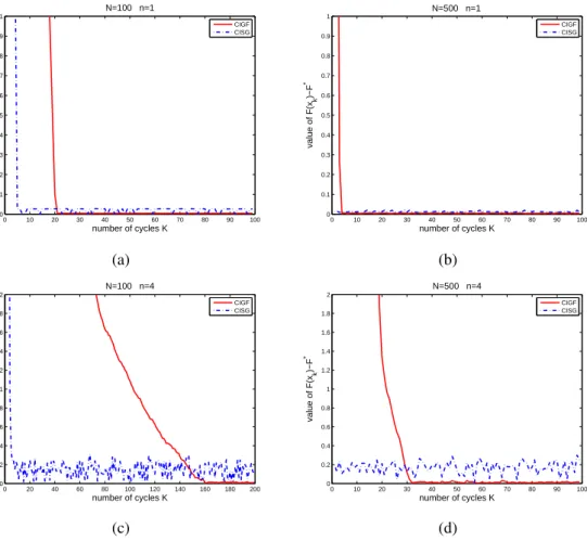
2.1. Function value error versus number of cycles K with a constant stepsize α= 0.001.. . . 55 2.2. Function value error versus number of iterations Kr a constant stepsizeα=
0.001. . . . 56 2.3. (a) Function value error versus number of cycles K with diminishing
step-size choices: α1(k) = 1/(m(k−1) +i), α2(k) = 1/(m(k−1) +i) 2 3, k =
0,1, . . . , i = 1, . . . , m; (b) Function value error versus number of iterations Kr with diminishing stepsize choices: θ1(k) = 1/k, θ2(k) = 0.1/k
2 3, k =
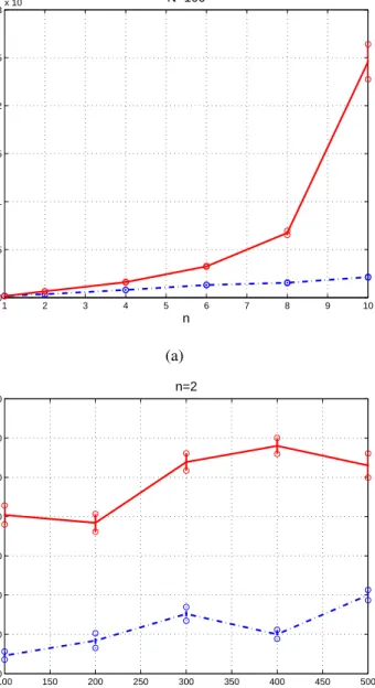
1,2, . . .. . . . 57 2.4. For a fixed target accuracy ϵ = 0.01 and a constant stepsize α = 0.001,
(a) number of iterationsKc versus dimension of the agentn; (b) number of
iterationsKc versus number of agentsN. . . 58
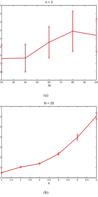
2.5. Max error versus number of iterations withN = 100 . . . 73 2.6. Max error versus number of iterations withN = 500 . . . 74 2.7. (a) number of iterations required to reach a fixed accuracy ϵ (vertical axis)
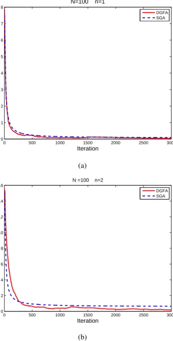
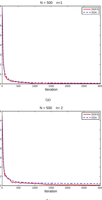
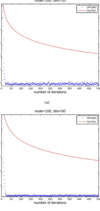
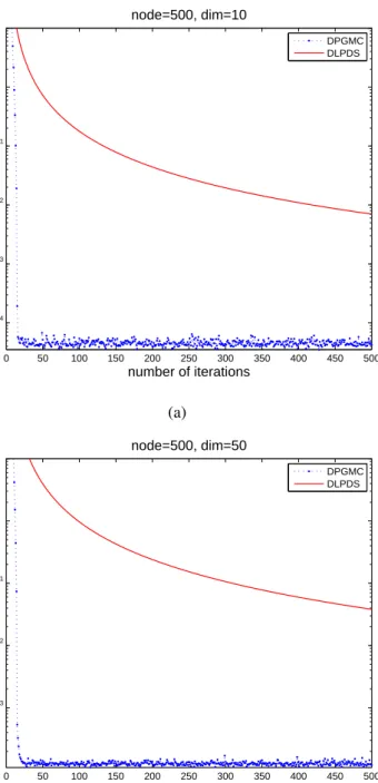
versus network size N (horizontal axis) for fixed n = 2; (b) number of iterations versus dimensions of the agentnfor fixed network sizeN = 20 . 75 3.1. Max error versus number of iterations with different dimensions forN = 100 100 3.2. Max error versus number of iterations with different dimensions forN = 500 101
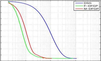
4.1. Total power consumption and capacity required for F-DFGP and M-DFGP . 133 4.2. Aggregated utility of all users for FPA, F-DFGP and M-DFGP . . . 133 4.3. For the usersN = 100, (a) value of primal objective function versus number
of iterations; (b) reference price of electricity versus number of iterations; (c) aggregated load level of all users and capacity required from the energy provider versus number of iterations. . . 135 4.4. For the usersN = 500, (a) value of primal objective function versus number
of iterations; (b) reference price of electricity versus number of iterations; (c) aggregated load level of all users and capacity required from the energy provider versus number of iterations. . . 136 4.5. Results of Algorithm IDFGP for ϵ=5e-3 with different inner accuracy: (a)
primal suboptimality versus number of outer iterations; (b) constraint viola-tion versus number of outer iteraviola-tions . . . 158 4.6. Results of algorithms IDFGP and IDFG withϵ=5e-3: (a) primal
suboptimal-ity versus number of outer iterations; (b) constraint violation versus number of outer iterations . . . 159 5.1. Objective value and maximum value of constraints violation versus number
of iterations on a random network with 20 sources and 50 links. . . 184 5.2. Number of iterations for both algorithms implemented over 50 randomly
generated networks withL ∈ [20,50]andS ∈[10,20]. . . 185 5.3. Number of iterations for both algorithms implemented over 50 randomly
Introduction
In the modern age, our world has become more and more connected through infrastruc-tures such as wireless network and Internet. A common feature of these systems is that they are composed of many subsystems that are interconnected through certain protocols. This class of system is referred to as network system and their subsystems are referred to as agents. In such multi-agent network there may be a multitude of agents who are decision makers yet, none of which possess all relevant information. Often the information to be processed is only known by single agent. On the other hand, some computation platforms have become increasingly decentralized. For example, computers are now equipped with several processors, allowing for parallel computation. Also, complex network systems such as power grid systems are composed of several interconnected subsystems, each with some processing power, and thus are distributed by nature.
All these factors have motivated much interest in designing decentralized algorithms that relies only on local information over a multi-agent network. However, it is challenging. Part of the reason is that efficient centralized algorithms, such as interior-point methods, cannot be easily adapted to decentralized scenarios. How to design high-level decentralized algorithms for solving optimization problems has become a research topic in the recent years.
Many problems associated with a multi-agent network possess the special structure, which have been taken considerable attention into optimization community. Among them, we are especially concerned with two prototypes, including multi-agent convex optimization (MCO) and separable convex optimization (SCO). In the problem (MCO), the network
ob-jective is that the agents cooperatively solve a global optimization problem through local computations and information exchange over a network. This class of problems has the characteristic that the global objective function is an additive form of many-terms compo-nent functions, which each agent has only access to its private compocompo-nent function but share a global decision vector. It arises in many network applications, including in-network esti-mation, machine learning and signal processing. The other class of the problem (SCO) has the characteristic that the objective function is separable in the decision vector, which each agent has only access to its private component function but the components of the decision vector are often coupled as constraints. It is quite general arising in diverse applications, including network resource allocation, and distributed model predictive control.
Considering the structure of problems and privacy of local objective functions, special optimization methods are always desirable for both theory research and engineering applica-tions, especially for large-scale structured problems.
In the literature there exist several useful techniques for solving the problem (MCO) in a distributed manner. In terms of the update strategies, they can be classified as the incremen-tal based approach and the consensus based approach. Most of these methods are based on the assumption that the subgradients of objective functions are available and easy to eval-uate. However, there exist a large number of problems where the subgradient information is unavailable or costly to compute. Typical examples often appear in stochastic program-ming. Moreover, for many practical engineers, derivative-free methods are always preferred because the input of subgradient requires the knowledge of convex analysis. In addition, subgradient-based methods may suffer from the slow convergence since an arbitrary anti-subgradient direction does not guarantee the decrease of the function value. Thus, in the distributed setting, the development of derivative-free optimization schemes attracts many research interests.
interconnected chemical process subject to certain physical constraints, are modeled as the problem (MCO) with equality and (or) inequality constraints. Methods available for solving these problems are still limited in the literature. These methods are mainly based on the Lagrangian duality and consensus averaging scheme, and there is no estimate on the conver-gence rate. Due to introducing Lagrangian multipliers, there is an obvious increase in the dimensions of solutions.
The alternating direction method of multipliers (ADMM) is suitable to solve the problem (SCO) with equality constraints using the augmented Lagrangian method. ADMM performs well in earlier iterations, but is slow to converge to high accuracy. The work on ADMM is still limited with the more general case when the number of separable blocks are greater than two.
Dual decomposition methods are powerful tools for solving the problem (SCO). They are based on the Lagrangian duality, since the coupling constraints can be moved into the cost function using Lagrange multipliers and then the primal subproblems with simple constraints are solved in parallel and the dual variables are updated with first-order methods. However, the dual problem is, in general, nonsmooth. Thus, the use of subgradient-based methods seems to be inevitable. It is well-known that subgradient-based methods have the slow con-vergence rate and are numerically sensitive to stepsize. Hence, there is a sustained effort in devising algorithms that have faster convergence rate and more robustness.
There is an additional issue for dual decomposition methods that they often involve in find-ing the exact solution of an inner subproblem at each iteration. However, from a practical point of view, the subproblem is never solved exactly. What will happen for dual decom-position methods when the inner subproblems are solved inexactly, thus, this is worthy of consideration.
Motivation
Despite the widespread use of distributed and parallel optimization methods mentioned above for solving structural problems, there are some aspects of these methods that have not been fully studied. In particular, the previous work has several limitations:
(1) Existing distributed methods are mainly based on the assumption that subgradients of objective functions are available and easy to evaluate. In distributed setup, there is no con-sideration when the subgradient information is unavailable or prohibitive.
(2) Existing distributed methods available for solving the problem (MCO) with global in-equality and (or) inin-equality constraints are limited in the literature. Moreover, there is no estimate on the convergence rate.
(3)Dual subgradient-based methods have the slow convergence rate. There are limited re-sults on convergence rates for dual gradient-based methods, while solving exactly the inner subproblems.
(4) There are limited results on convergence rates for dual gradient-based methods, while solving inexactly the inner subproblems.
All these limitations motivate our work in this thesis.
Contributions of the thesis
The main purpose of this thesis is the development of efficient decentralized algorithms and the convergence rate analysis of these proposed algorithms. We are specially interested in two classes of structured convex optimization problems, which arise in a variety of prac-tical applications.
We now describe the contributions of the thesis in more detail:
Chapter 2.In this chapter, we develop distributed gradient-free methods for the problem (MCO) with simple constraints, including an incremental gradient-free method and a consen-sus gradient-free method. The convergence analysis and convergence rates of the proposed
methods are provided. Extensive numerical results are illustrated. By comparison, existing distributed algorithms require first-order information of objective functions, but our methods only involve the estimates of objective function values. Therefore, the proposed methods are suitable to solve more general problems even when the first-order information of problems is unavailable or costly to compute. The distributed consensus-based gradient-free method in this chapter is based on the publication [J1].
Chapter 3.In this chapter, we develop a distributed proximal-gradient method for solving the problem (MCO) subject to global inequality constraints by using the exact penalty func-tion method and multi-consensus scheme. We establish the convergence rates of the method, depending on number of iterations, the network topology and number of agents. Simula-tion experiments on a distributed state estimaSimula-tion problem illustrate the performances of our proposed method. The method is different from existing distributed primal-dual consensus methods, not involving Lagrangian multipliers. This chapter is based on the publication [J2].
Chapter 4. This chapter is divided into two parts. In the first part, we develop a fast gradient-projection method for solving the problem (SCO) when the inner subproblem is solved exactly. In the sense of averaging, we show that the computational complexity bound of the method for achieving anϵ-optimal feasible solution is O(1/ϵ). To further accelerate the proposed algorithm, we modify it by using a restart technique. The advantage of our algorithm is fast, parallelizable and allows us to simultaneously obtain the dual solutions and primal solutions. The proposed algorithm is applied to a real-time pricing problem for smart grid. Numerical experiments illustrate the effectiveness of the proposed algorithms. This part is based on the work [J3].
In the second part, we extend the fast dual gradient-projection method to the situation when all inner subproblems are solved inexactly. We prove the convergence of the proposed algorithm. In particular, we provide explicit convergence rates on the dual suboptimality, primal suboptimality and primal infeasibility of the generated approximate solutions.
Nu-merical simulations are presented to illustrate the effectiveness of the proposed algorithm. The advantage of the algorithm is allows us to solve the inner subproblems up to a certain precision while still maintaining the same iteration complexity as the exact counterpart. The results of this part is based on the work [C3].
Chapter 5. In this chapter, we develop a fast dual gradient method for solving the prob-lem (SCO) with linear constraints based on Nesterov’s smoothing technique and a simple fast gradient scheme. We show that the computational complexity bound of the method for achieving anϵ-optimal feasible solution is O((1/ϵ) ln(1/ϵ)). By comparison, the iteration complexity of the proposed method is at most a factorO(ln 1/ϵ)worse than that of the fast dual gradient-projection method. But the method is simpler and we do not need any running average of sequences of dual and primal solutions. This chapter is based on the work [J4].
The remainder of the thesis is organized as follows. In Chapter 1, a literature review closely related to this thesis is given. In Chapter 6, some remarks and recommendation for future work are given.
Chapter 1.
Literature review
The history of decentralized optimization is only a few decades old but has attracted an extensive research interest in recent years. In contrast to the centralized optimization coun-terparts, they offer several advantages, for examples, the ability to process distributed data, easy collaboration with neighbors, enhanced reliability and availability. In the context of op-timization, research on parallel methods, including decomposition methods, date back to the sixties with the works of Dantzig and Wolfe [30], Benders [12], and Everett [39]. Distributed methods started later, in the mid-eighties, with the work of Tsitsiklis, Bertsekas, and Athans [123] and has boomed in the past ten years, motivated by the widespread of networks.
In this chapter, we first overview the convex optimization with special structure includ-ing multi-agent convex optimization and separable convex optimization, then we overview existing work on distributed and parallel optimization methods for solving these structured problems under consideration.
1.1. Structural convex problems
We focus on the following form of structural problems:
(SCP) min f(x) := N ∑ i=1 fi(xi) s.t. (x1, . . . , xN)∈C,
where(x1, . . . , xN)is a vector inRn1+···+nN with componentsxi ∈ Rni, i = 1, . . . , N, and
Cis a constrained set inRn1+···+nN.
We are interested in the case when fi(xi) : Rni → R is a convex function for each i
andC is a convex subset ofRn1+···+nN. Thus, the above problem belongs to the context of
convex optimization. Here we refer to it as structural convex programming (SCP, for short). In particular, when all theni = 1, the minimization problem (SCP) is called as monotropic
programming, which was introduced and extensively analyzed by Rockfellar [104]. In his recent book [16], Bertsekas generalizes the monotropic programming to a more general case, termed as the extended monotropic programming. In this thesis, we focus on two special cases of problem (SCP) arising in many applications.
Multi-agent convex problems
By letting all thexi be equal toxand the subspace C = {(x, . . . , x)|x∈ X}in problem
(SCP), an important class of problems can be obtained as follows:
min f(x) := N ∑ i=1 fi(x) (1.1) s.t. x∈X,
wherefi(x) : Rn → Ris a convex function for each i, and X is a subspace of Rn. This
class of problem (1.1) has the characteristic that the cost functionf(x)is additive and all component functionsfi(x)share a global decision vector x. Problem (1.1) is often termed
multi-agent convex optimizationor distributed convex optimization[20, 79, 36], and arises in many network applications, including in-network estimation, machine learning, signal processing, resource allocation, and distributed model prediction and control [17, 99, 111, 130, 72]. For such applications the numberN of component functions may be very large, in which case special methods that take advantage of the additive structure of the cost are desirable.
We provide two such applications, including the parameter estimation problems in sensor networks andl1-regularization problems.
Parameter estimation problems in sensor networks. A typical problem involving the additive structure is the parameter estimation problem in a sensor network. This consists in finding a set of parameters or functions of interest that best fits a certain criterion based on the measurements collected by the sensors. For example, we consider a network withN sensors and assume that each sensoricollects a set ofM measurements(θi1, . . . , θiM). Now we aim to estimate a common parameterxaccording to these measurements. For example, our objective is to compute the average value of all the measurements. In particular, many estimation criteria possess the following form:
f(x) = 1 N N ∑ i=1 fi(x),
where x is the parameter to be estimated, and f(x) is the cost function which can be ex-pressed as a sum ofN local functionsfi(x), in whichfi(x)only depends on the data
mea-sured by sensori. In the average case, we often have fi(x) = 1 M M ∑ j=1 ||x−θij||1 orfi(x) = 1 M M ∑ j=1 ||x−θij||2.
Hence the parameter estimation problem in sensor networks can be recast to the form of problem (1.1). We can refer to the literature [98, 111] for more details.
l1-regularization problem. In data analysis and machine learning, many problems usu-ally involve an additive cost function, where each termfi(x)corresponds to error between
data and the output of a parametric model, withxbeing a vector of parameters. A classical example is least squares problems, wherefi has a quadratic structure. A regularization
func-tion is often added to the least squares objective. Recently, nondifferentiable regularizafunc-tion functions have become increasingly important. For example, the followingl1-regularization problem, min x∈Rn N ∑ i=1 (aTi x−bi)2+γ||x||1,
which arises in statistical inference and image processing. Note that the term||x||1 is used to induce the sparsity of the solution. There are several interesting variations of the l1-regularization approach with many applications, for which we refer to the literature [16, 5, 70, 69]. Thel1-regularization problem can be posed in the form of problem (1.1) by letting fi(x) = (aTi x−bi)2+γ||x||1/N.
Separable convex problems
Next we introduce two typical examples which can be viewed as a special case of the problem (SCP).
Network utility maximum problem.Utility maximum problem is a classical problem in network optimization. The problem is characterized by a fixed network and a set of sources
source has a local utility function over the rate xs which it sends information. Denote the
rate vector by x = [xs], s ∈ S and the link-source incidence matrix by A. The goal is
to determine the source rates that maximize the sum of utilities subject to link capacity constraints [58, 66, 115]:
max f(x) :=∑
s∈S
Us(xs)
s.t. Ax≤c, xs ∈Is,
where the utility functionUs is often concave and only known by resource s. Note that the
explicit structure of the cost functionf(x) is separable in the components of the decision vectorx. Moreover, the global constraint setC = {x|Ax≤ c, xs ∈Is}is given by the link
capacity constraints and local constraint setsIs. Thus, network utility maximum problems
fall into the class of problem (SCP).
Network minimum cost problem. Consider a network represented by a directed graph
G = (N,E) with node setN and edge setE. Denote the flow vector by x = [xe], e ∈ E,
wherexe denotes the flow on edgee. The flow conservation conditions at the nodes can be
compactly expressed asAx = c, where Ais the node-edge incidence matrix of the graph. Each edge e is equipped with a convex cost function ϕe (only known by this edge). The
problem [20, 53] can be written as follows:
min f(x) :=∑
e∈E
ϕe(xe)
s.t. Ax=c.
Clearly, the network minimum cost problem, involving a separable convex cost function and linear equality constraints, can be also converted to the problem (SCP).
problem considered in this thesis: min x f(x) := N ∑ i=1 fi(xi) (1.2) s.t. N ∑ i=1 Aixi −b ≤0 = 0 , xi ∈Xi, i= 1, . . . , N,
where fori = 1, . . . , N, fi : Rni −→ Ris convex,Xi ⊂ Rni is a nonempty closed convex
set, Ai ∈ Rm×ni, and b ∈ Rm. x = (xT1, . . . , xTN)T with xi ∈ Rni, i = 1, . . . , N and
n1+n2+· · ·+nN =n.
Note that the problem (1.2) is a special form of problem (SCP), which has the character-istic that the cost function isseparable in the decision vectorxand the components of the decision vector x are linearly coupled as constraints. This class of problem (1.2) is often termedseparable convex optimization, which is quite general arising in diverse applications. Except for network utility maximum problems and minimum cost problems, many others problems including distributed model predictive control [73, 38, 95], real-time pricing prob-lems for smart grid [108, 109], the optimal power flow probprob-lems for a power system [139], can also model this class of problems.
Related to the problems above, we are concerned with two types of optimization meth-ods to solve them over a multi-agent network, including distributed methmeth-ods and parallel methods.
An optimization method is considered distributed if it shares two characteristics: (i) the information associated with each agent is processed locally; (ii) no central agent coordinates the network and all the communications occur only between neighboring agents. An opti-mization method that satisfies the first characteristic but not the second one is usually called a parallel method. According to [20], parallel methods run on systems where computing
devices are at a small distance of each other and may be controlled by a central entity. Dis-tributed methods, in contrast, run on systems where computing devices are located far apart, making centralized coordination inconvenient.
1.2. Distributed optimization methods
In this section we review existing distributed optimization methods, designed for solving problem (1.1). Since no central coordinator has the ability to access to all the information in problem (1.1), centralized methods are often unavailable. In the literature, there exist several useful techniques for solving problem (1.1) in a distributed manner. In terms of the update strategies, most of them can be classified as the incremental based approach [113, 75, 76, 19, 59] and theconsensus based approach[79, 82, 100, 36, 138].
Incremental-based methods
For solving the problem (1.1), the incremental (sub)gradient method behaves with the same scheme as the classical (sub)gradient method. However, instead of using the full (sub)gradient of the cost functionf1+· · ·+fN, it only uses the (sub)gradient of one function
fi at each iteration [113, 76, 16]. More specifically, the update consists of
xk+1 = ΠX[xk−αkgik(xk)], (1.3)
wheregik(xk)is the (sub)gradient of component functionfik atxk, αkis a positive stepsize
chosen suitably andΠX denotes the Euclidean projection onto the setX. The sequence{ik}
takes values in{1, . . . , N}and determines the order of the updates, which can be determin-istic or randomized.
Incremental methods are surveyed, including convergence analysis and convergence rate analysis, by Bertsekas in his recent book [16]. The methods have been very successful
in solving parameter estimation in networks of wireless sensors [99, 111], stochastic pro-gramming [37]. In terms of the strategies that the sequence{ik}is selected, most of existing
incremental based approach can be classified into ascyclic incremental methods[76, 17, 18], equiprobable randomized incremental methods[76, 17, 18], andMarkov randomized incre-mental methods[57, 101]. In [76], the authors developed the cyclic incremental subgradient method and a new equiprobable randomized incremental subgradient method for distribution optimization, and provided the convergence and convergence rate analysis. Unlike the cyclic incremental method, the authors have extended the equiprobable randomized incremental subgradient method to a more general case where the sequence{ik}is selected in a time
ho-mogeneous Markov chain [57] or a time nonhoho-mogeneous Markov chain [101]. The recent work [17] surveys these methods and, in addition, presents a unified view of incremental (sub)gradient methods, incremental proximal methods, and their combination.
In general, incremental (sub)gradient methods progress simpler and faster than their non-incremental counterparts far from the solution, but are slower near the solution [17]. Since they use the (sub)gradient of only the component function at each iteration, they can be im-plemented naturally in a distributed manner, with a single agent performing the update (1.3) at each iteration. The disadvantage of incremental (sub)gradient methods is that they have the slow asymptotic convergence rate not only because they use subgradient-based meth-ods, but also because they require a diminishing stepsize for convergence. If the stepsize is instead taken to be constant, an oscillation arises.
Consensus-based methods
In the consensus based approach, the agents (nodes) achieve the minimizer globally through sharing the information locally (the agent only shares information with its neighbors). The implementations of the consensus strategy relies on the use of two scales: one time-scale for the collection of measurements across the agents and another time-time-scale to iterate
sufficiently enough over the collected data to attain agreement before the process is repeated [82, 79] until optimization is achieved. There are two different types of strategies in the second time scale: the synchronous strategy and the asynchronous strategy.
Average consensus scheme [131, 132] has triggered the increasing interest on the design of distributed methods for problem (1.1), since distributed methods have the motivating ap-plications in sensor networks [98]. The important pioneer work includes subgradient-based distributed algorithms by Nedi´c et al. [77, 79, 80, 82, 100], whose work was inspired by [124, 123].
Consensus averaging. The consensus averaging algorithm consists in computing the av-erage of states distributed among the multiple agents in the network in a distributed and iterative fashion. The consensus algorithm means that each agent in the network gets its state updated by using its own and its neighboring agents’ states, i.e., for each agenti
xki+1 = ∑
j∈N(i)
Wijxkj, (1.4)
whereN(i) represents the neighbors of agent iincluding itself, the weight matrix [Wij] is
often assumed to be a doubly stochastic matrix. Xiao et al. [132] have proved that the consensus averaging algorithm enforces that all the agents’ states converge to the average of their initial states, and the convergence rate of the consensus algorithm is determined by ρ(W − 1
N11
T)(the notationρ(·)denotes the spectral radius).
In terms of consensus manners, we can classify existing consensus-based distributed ap-proaches into three classes: primal consensus distributed methods (the consensus strat-egy directly enforces all estimates of primal variables to an agreement on the optimum) [56, 79, 82, 100], dual consensus distributed methods (the consensus strategy enforces all estimates of dual variables to an agreement on the optimum) [36, 122, 121] andprimal-dual consensus distributed methods(the consensus strategy simultaneously enforces all estimates of primal and dual variables to an agreement on the optimum) [138, 136, 135]. Next we
overview them respectively.
Primal consensus distributed method. The primal consensus distributed method based on (sub)gradients is formally written as follows [79]:
zki+1 = ∑
j∈N(i)
Wijzjk−αkgi(zik) and x k+1
i = ΠX[zik+1], (1.5)
where gi(zki) is the (sub)gradient of local function fi at zki, αk is a positive stepsize and
ΠX[x] := arg minx∈X{||y−x||}is the Euclidean projection onto the set X. Note that the
pointzk
i is nothing but an intermediate parameter just for convenient comparison with the
dual consensus methods later. For more compact form we can refer to [79, 100]. At each iterationk, agent i receives the estimates zk
j from its neighbors j ∈ N(i), averages them
with its own estimate zk
i, and then performs a projected (sub)gradient update, where the
(sub)gradient that is used is the one given by its private functionfi. The role of consensus
averaging is to bring all the estimates of primal variablesxi to an agreement. Observe that
when all local functions fi = 0 and the set X are the entire space Rn, (1.5) reduces the
consensus averaging algorithm (1.4); and when the network is reduced to a single node, (1.5) becomes the traditional (sub)gradient algorithm.
In [79], the convergence of algorithm (1.5) for solving unconstrained distributed opti-mization problem has been established for the first time over a time-varying connectivity structure. The work in [100] has analyzed a projected distributed subgradient algorithm for problem (1.1). Variations of algorithm (1.5) have also been explored [56, 82]. For example, in [56], the authors have surveyed a multi-consensus version. The work by [79, 100] pro-vided a much tighter analysis that yields the convergence rates that scale polynomially in the number of agents in the network, but they are independent of the network topology [36].
Dual consensus distributed method.The dual consensus distributed method is based on a projected dual averaging algorithm [89, 130]. Duchi et al. [36] extended the projected dual averaging algorithm to the distributed setting and proposed a distributed dual averaging
algorithm. Since the consensus averaging strategy is used to bring all the estimates of dual variables to an agreement rather than the estimates themselves, we also call it as a dual consensus distributed algorithm. At each iterationk, the algorithm maintains pairs of vectors
(xk
i, zik)and the updates are performed as follows [36]: for each agenti,
zik+1 = ∑ j∈N(i) Wijzjk+gi(zik) and xki+1 = Π ψ X[z k+1 i , αk], (1.6)
wheregi(zik)is the (sub)gradient of local functionfiatzik,αkis a positive stepsize. Here the
projectionΠψX is defined asΠψX[z, α] := arg minx∈X{zTx+21αψ(x)},whereψis a 1-strongly
convex function, which can viewed as a proximal projection onto the setX. In words, for algorithm (1.6) agent i computes the new dual estimate zik+1 from a weighted average of its own subgradientgi and the estimates{zjk, j ∈ N(i)}in its own neighborhood, and then
computes the next local iteratexki+1 by a proximal projection with a stepsizeαk. The work
[36] has shown that the number of iterations required by algorithm (1.6) scales inversely in the spectral gap of the network. The authors in [122] considered the communication delay based on the dual consensus distributed algorithm.
Both algorithms (1.5) and (1.6) are based on the consensus averaging scheme, which have the advantage of making all agents active and communications with neighbors at each it-eration. By comparison, however, the dual consensus distributed algorithm (1.6) is quite different from the primal consensus distributed algorithm (1.5). First, the consensus aver-aging strategy is used to bring all the estimates of dual variables to an agreement rather than the estimates of primal variables. Second, a more general proximal projection with non-Euclidean geometry is used in the dual consensus distributed algorithm (1.6) while the Euclidean projection is used in the primal consensus distributed algorithm (1.5). Finally, the convergence analysis of both algorithms is also distinct (see e.g., [79, 100, 36]).
Primal-dual consensus distributed methods. The primal-dual consensus distributed method is designed for solving the problem (1.1) with global inequality constraints under
the framework of Lagrangian duality. Consider the following problem: min x∈X f(x) := N ∑ i=1 fi(x) (1.7) s.t. gs(x)≤0, s= 1,2, . . . , p,
wheregs : Rn → R, s = 1,2,· · · , p, are the global inequality constraints known by all the
agents in the network. Define the Lagrangian function for problem (1.7) as
L(x, λ) = N ∑ i=1 fi(x) +λTg(x) = N ∑ i=1 Li(x, λ),
whereλ ∈ Rp+ is the vector of dual variables, g(x) = (g1(x), . . . , gp(x))T and Li(x, λ) =
fi(x) +λTg(x)/N. Based on the characterization of the primal-dual optimal solutions as
the saddle points of the Lagrangian function, Zhu et al. [138] first proposed the primal-dual consensus distributed algorithm:
zik+1 =∑j∈N(i)Wk ijxkj, µ k+1 i = ∑ j∈N(i) Wijkµkj, xki+1 = ΠX[zik+1−αkgi1(zik+1, µ k+1 i )], λ k+1 i = [µ k+1 i +αkgi2(zik+1, µ k+1 i )]+, where gi1(zik+1, µ k+1 i ) ∈ ∂1Li(zik+1, µ k+1 i ) and gi2(zki+1, µ k+1 i ) ∈ ∂2Li(zik+1, µ k+1 i ). The
algorithm involves each agent updating its estimates of the saddle points via a combination of an average consensus step, a subgradient step and a primal (or dual) projection step onto its constraint set. Unlike algorithms (1.5) and (1.6), the consensus averaging is simultaneously acted on the estimates of primal and dual variables. In [138], the authors have proved that the algorithm asymptotically converge to a pair of primal-dual optimal solutions under the Slater’s condition and the periodic strong connectivity assumptions. Variants of the primal-dual consensus distributed algorithm have been discussed in [136, 135].
global equality and inequality constraints by assorting to Lagrangian duality. However, the drawback of this method is the increase of variables due to introducing Lagrangian multiplier. In addition, there is no convergence rate available up to now.
In conclusion, incremental-based methods and consensus-based methods are distributed with each agent only involving its private cost function. But they are different in distributed fashions. In incremental methods, only one agent updates at each iteration, whereas in dis-tributed methods, every agent operates and maintains an estimate of the global optimum. Moreover, incremental methods relies on a cyclic or uniformly random order of passing the iterate, while distributed methods consider more generic communication networks in which the agents pass iterates to multiple neighboring agents, and also combines the estimate re-ceived from different agents.
1.3. Parallel optimization methods
We start by reviewing several methods that work as building blocks of parallel implemen-tation. These methods are mainly decomposition methods, alternating direction method of multipliers and block-coordinate minimization methods.
Decomposition methods
Decomposition methods in optimization have a long history and derive from the early 1960s, see the well-known work by Dantzig and Wolfe [30] and Benders [12] on large-scale linear programming. Good references on decomposition methods include the books by Bertsekas [20, 15] and by Boyd [23]. Some recent references on decomposition applied to networking problems are Kelly et al. [58], Palomar et al. [93] and Chiang et al. [28]. The basic idea is to decompose a complex problem into smaller, simpler ones in parallel or sequentially. However, they are not regarded as distributed, because they generally require a master agent coordinating several slave agents. Most of existing decomposition methods
can be divided intoprimal decomposition methods and dual decomposition methods. The former indicates that the optimization problems are solved using the original formulation and variables, whereas the latter indicates that the original problem has been rewritten using Lagrangian relaxation. Next we overview them to solve problem (1.2), respectively.
Primal decomposition. To solve problem (1.2) via primal decomposition, we rewrite it as min y1,...,yN g1(y1) +· · ·+gN(yN) (1.8) s.t. y1+· · ·+yN ≤ (or =)b, yi ∈Yi, i= 1, . . . , N,
where eachyi ∈Yi ⊆Rmandgi :Rm →Ris defined as
gi(yi) := min xi∈Xi
fi(xi) (1.9)
s.t. yi =Aixi.
Given a master agent andN slave agents, the master agent solves the master problem (1.8) in charge of updating the coupling variable yi, while slave agent i solves the decoupled
subproblems (1.9) in parallel. In general, the master problem (1.8) is solved with first-order methods, such as subgradient-based methods. It can be shown that the subgradient of gi
at a point yi is given by −λi, where λi is the dual optimal solution corresponding to the
constraint of (1.8); see [15] for more details. Therefore, in primal decomposition, the master agent updatesy= (y1, . . . , yN)T as
yk+1 = ΠY[yk+αkλk], (1.10)
At each iteration, the master agent sendsyi to slave agenti, who then solves the problem in
(1.9) and returns λki to the master agent. The master agent, in turn, updates y as in (1.10) and moves on to the next iteration. Note that primal decomposition is not distributed since it requires a master agent playing the role of a central coordinator.
Dual decomposition. By considering the special structure of problem (1.2), the dual decomposition method is motivated by the dual ascent method [22]. Dual decomposition methods, rather than solving problem (1.2) directly, solve dual problem instead. For simplic-ity, we consider problem (1.2) with equality constraints. In this case, lettingλ ∈Rm be the dual variable, the Lagrangian function for problem (1.2) is
L(x, λ) = N ∑ i=1 Li(xi, λ) = N ∑ i=1 [fi(xi) +λTAixi−λTb/N],
which is separable inx. Therefore, the dual problem becomes
max
λ d1(λ) +· · ·+dN(λ), (1.11)
where eachdi(λ) :Rm →Ris defined as
di(λ) = min xi∈XiL
i(xi, λ) = min xi∈Xi{
fi(xi) +λTAixi−λTb/N}. (1.12)
It is interesting that the Lagrangian dual of separable convex problem (1.2) is a distributed convex problem like problem (1.1). In addition, assuming that all the functionsfiare convex,
when the dual problem is dualized, it yields the primal problem, and the duality is fully symmetric [16].
Given a master agent and N slave agents, the master agent solves the master problem (1.11) while slave agentisolves subproblems (1.12). Whenever each functionfi is strictly
of the problem in (1.12) for a givenλ. Hence, in this case, after the master agent finds a dual solutionλ∗ to problem (1.11), the ith block of the optimal primal solution of problem (1.2) can be found in theith slave agent as xi(λ∗). In other words, when each function fi
is strictly convex, a primal solution is immediately available after solving the dual problem (1.11). Again, the master problem (1.11) can be solved with first-order methods, such as subgradient-based methods. The subgradient ofdi(λ) at a pointλ isAixi(λ), where xi(λ)
solves the problem in (1.12) [15]. Hence, in dual decomposition, the master agent updatesλ as λk+1 =λk+αk[ N ∑ i=1 Aixi(λk)−b]. (1.13)
At each iteration, the master agent sendsλkto all slave agents and each slave agenti, in turn, returnsAixi(λk)to the master agent. Similarly to primal decomposition, dual decomposition
also requires the master agent as a central coordinator and, therefore, it is not distributed. Finally, the dual decomposition algorithm is summarized as follows:
xki+1 = argmin xi∈Xi Li(xi, λ), i= 1, . . . , N, λk+1 = λk+αk[ N ∑ i=1 Aixki+1−b],
For eachi = 1, . . . , N, the xi-minimization step is carried out independently, in parallel.
Sometimes, we refer to it asLagrangian dual decomposition. There also exist other dual de-composition techniques, including the Dantzig-Wolfe dede-composition [30, 15] and the Ben-ders decomposition [12].
Alternating direction method of multipliers
The alternating direction method of multipliers (ADMM, for short) can solve problem (1.2) with equality constraints using the augmented Lagrangian method. For simplicity, we consider the case whenN = 2in the following form:
min
x1,x2
f1(x1) +f2(x2) (1.14) s.t. A1x1+A2x2 =b,
where fori = 1,2,fi : Rni −→ Ris convex, Ai ∈ Rm×ni is full column rank matrix. The
augmented Lagrangian function of problem (1.14) is
Lρ(x1, x2;λ) = f1(x1) +f2(x2) +λT(A1x1+A2x2−b) + ρ
2||A1x1+A2x2−b||
2,
whereλ is the dual variable and ρ is a positive penalty parameter. ADMM minimizesLρ
first with respect tox1, then with respect tox2, and it finally updates the dual variableλ:
xk1+1 = arg min x1 Lρ(x1, xk2;λk), (1.15) xk2+1 = arg min x2 L ρ(xk1+1, x2;λk), (1.16) λk+1 = λk+ρ(A1x1k+1+A2xk2+1−b). (1.17)
ADMM can be considered as an application of the method of multipliers [15], but they are different with the update of primal variables. In the method of multipliers for problem (1.14), it minimizesLρjointly with respect to the primal variables(x1, x2)as(xk1+1, xk2+1) =
arg min(x1,x2)Lρ(x1, x2;λ
k), whereas, in ADMM, the minimization ofL
ρwith respect to the
primal variable(x1, x2)consists of just oneGauss-Seidelpass, see (1.15) and (1.16).
and Gabay and Mercier [41]. The convergence of ADMM has been explored by many researchers, including Gabay [40] and Eckstein and Bertsekas [63]. A recent survey on ADMM is given by Boyd et al. in [22]. The work that establishes the convergence rates for modified versions of ADMM includes [44, 50, 48] and references therein. The recent interest on ADMM has been extensively motivated by its application in many areas, such as image processing, statistical and machine learning problems [22]. Under the strong convexity as-sumption on the component functionfifor problem (1.2), Han et al. proved the convergence
of ADMM for the case whenN >2by using the tool of variational inequalities [46]. How-ever, the work on ADMM is still limited with the more general case whenN > 2andfi is
convex in problem (1.2) [48, 46, 47]. Numerical examples show that ADMM performances well in the earlier iterations, but is slow to converge to high accuracy [22]. In practice, the performance of ADMM is significantly affected by the penalty parameterρ, which is adapted by heuristics.
Block coordinate descent methods
Block coordinate descent (BCD, for short) methods are appropriate in contexts where the cost function and constraints have a partially decomposable structure with respect to the variables for the optimization problems under consideration. Consider, for example,
min
x=(x1,...,xN)
f(x1, . . . , xN) (1.18)
s.t. x∈X1× · · · ×XN,
wherex = (xT
1, . . . , xTN)T ∈ Rn with xi ∈ Rni and n1 +· · ·+nN = n. We assume that
the cost functionf : Rn −→ R is convex, and each set X
i ⊆ Rni is closed and convex.
As working with all the variables of problem (1.18) at each iteration may be difficult or prohibitive, the variables are partitioned into manageable blocks, with each iteration focused
on updating a single block only, the remaining blocks being fixed, i.e.,
min
xi∈Xi
f(x1, . . . , xi−1, ξ, xi+1, . . . , xN), i= 1, . . . , N. (1.19)
Here it is necessary to assume that each subproblem above is easy to solve. There exist two important types of BCD methods, includingnonlinear Jacobiandnonlinear Gauss-Seidel.
Nonlinear Jacobi. Given the current iterate xk = (xk1, . . . , xkN)T, the nonlinear Jacobi method generates the next iteratexk+1 = (xk+1
1 , . . . , x k+1 N )T as follows: xki+1 = arg min xi∈Xi f(xk1, . . . , xki−1, ξ, xki+1, . . . , xkN), i= 1, . . . , N. Since updatingxk i tox k+1
i requires all the other block components to be fixed at xkj, j ̸= i,
the updates can be carried out in parallel.
Nonlinear Gauss-Seidel. Given the current iterate xk = (xk
1, . . . , xkN)T, the nonlinear
Gauss-Seidel method generates the next iteratexk+1 = (xk+1 1 , . . . , x k+1 N )T as follows: xki+1 = arg min xi∈Xi f(xk1+1, . . . , xki−+11, ξ, xki+1, . . . , xkN), i = 1, . . . , N.
In contrast with Jacobi methods, updatingxi at iterationk+ 1requires knowing the current
estimates of the first(i−1)blocks, i.e., xkj+1, j < i. Hence, all updates have to be carried out sequentially.
The results of convergence for BCD methods were studied extensively in the literature (see, e.g., [15, 117, 120] and the references therein). A renewed interest in BCD methods for large-scale problems was sparked recently by their successful applications in several areas, including training support vector machines [24], regression [129]. Randomized BCD methods become increasingly popular by the Nesterov’s work [91]. In [102], the authors extended them to the setting to the problem of minimizing a composite function, i.e., the sum of a smooth convex and a (possibly nonsmooth) convex block-separable functions.
The main advantages of the BCD method are two: (i) updating one or just a few blocks of variables are computationally much cheaper than the batch update; (ii) it is well suited for parallel computation [15]. However, there exist several shortcomings for BCD methods, for examples, (i) the algorithm is much slower near the optimum than more sophisticated meth-ods; (ii) if the single subproblem (1.19) is hard to solve, the BCD seems to be unavailable.
1.4. First-order optimization methods
Due to simplicity of computations per iteration, first-order methods have gained popularity in the last few years. In this section, we review several first-order methods for convex op-timization, including subbased methods for nonsmooth optimization and gradient-based methods for smooth optimization. In particular, we are interested in convergence rates of these methods.
Computational complexity issues
Suppose thatf : Rn → Ris a convex function andX ⊆ Rn is a closed convex set, we consider the following optimization problem:
min
x∈X f(x). (1.20)
We assume that there exists an optimal solution for problem (1.20). We focus on first-order algorithms that have good performance guarantees, in the sense that they require a relatively low number of iterations (in the worst case) to achieve a given optimal solution tolerance.
For any givenϵ >0, we want to estimate the number of iterations required by a particular algorithm to obtain a solution with cost that is withinϵ of the optimal. If we can show that
any sequence{xk}generated by a method has the property that for anyϵ >0, we have
inf
k≤N(ϵ)f(xk)≤f
∗+ϵ,
wheref∗is the optimal value of problem (1.20),N(ϵ)is a function that depends onϵ, as well as the problem data and the starting pointx0. We say thatxkis anϵ-optimal solution and the
method hasiteration complexityO(N(ϵ))to achieve anϵ-optimal solution [16].
The iteration complexity is characterized in terms of the number of iterations required to reach anϵ-optimal solution. For examples, the subgradient method for solving nonsmooth problem (1.20) has anO(1/ϵ2)iteration complexity [86]; the gradient method has anO(1/ϵ) iteration complexity when applied to smooth problem (1.20) with Lipschitz continuous cost gradient [86]. But the iteration complexity for the latter is not optimal [86]. In [84], Nesterov proposed an accelerated gradient method by employing an intricate extrapolation device, and has obtained the optimal iteration complexity ofO(1/√ϵ).
Next we distinguish two convergence notions between exact convergence and convergence to an error neighborhood [25].
For example, assume that a sequence{xk}
k≥0generated by a method satisfies f(xk)−f∗ ≤ C
k, (1.21)
for some scalarC >0. Letting the right-hand side of (1.21) toϵ, we see that it takes at most k = C/ϵ iterations to find an ϵ-optimal solution. We say that the iteration complexity of the method isO(1/ϵ). In this case, we also say that the method converges exactly, and the convergence rate isO(1/k).
Another type of convergence, which usually arises in methods that use a constant step size, involves terms that depend on the step sizeαand do not diminish askincreases. As an
example, we consider the bound
f(xk)−f∗ ≤ C1
αk2 +C2α, (1.22)
for some scalarsC1, C2 > 0. Under the characterization of ϵ-optimality convergence rate, if we first fix the number of iterationsk that this method is allowed to execute, then choose α=√C1/(k2C2)by minimizingC1/(αk2) +C2αwith respect toα, the bound becomes
f(xk)−f∗ ≤
√
C1C2 k .
Therefore, with a budget of k iterations, the best solution we can achieve is a √C1 C2/k-optimal solution. In other words, to reach an ϵ-optimal solution, at least k = √C1C2/ϵ iterations are required. In this case, sinceϵ=√C1C2/k, we say that the convergence rate of this method isO(1/k).
Although the convergence rates, e.g., see (1.21) and (1.22), are equal, the mechanism of the convergence between them is quite different. The expression (1.21) does not require fixing a budget of iterations in advance so as to find the optimal constant step size, and it approaches the optimal solution as the method continues to run for more iterations. On the other hand, once the constant step size is fixed, (1.22) does not reach the optimal solution even if the method continues for more iterations; however, in the early stages, the rate of de-crease in the function value is1/k2, and it may outperform than (1.21), until (1.21) decreases beyond the error neighborhood of (1.22). Therefore, as an alternative interpretation of con-vergence rate in the latter case, it is often helpful explicitly state the rate at which the error neighborhood is being reached. Taking (1.22) as an example, we also said that it converges to an error neighborhoodC2αwith rateO(1/k2).
Subgradient-based methods
Subgradient-based methods are principal methods for solving nonsmooth convex prob-lems (1.20). We review two important classes of methods based on subgradients, including subgradient projection methods and mirror descent methods.
Subgradient projection method. The update of a subgradient projection method is de-scribed as follows: xk+1 = ΠX[xk−αkgk] := arg min x∈X{g kTx+ 1 2αk ||x−xk||2}, (1.23)
wheregkis the subgradient of f atxk, i.e., gk ∈ ∂f(xk), Π
X[·]is the Euclidean projection
onto the setX, andαk >0is the stepsize chosen suitably.
The key advantage of the subgradient method is its simplicity. It seems like the ordinary gradient projection method for smooth convex optimization, but with several notable ex-ceptions. For examples, the subgradient method uses a single subgradient at each iteration, rather than the entire subdifferential; it can uses a constant stepsize, instead of an exact or inexact line search as in the gradient method. Unlike the gradient method, the subgradient method is not a descent method, that is, it does not guarantee that the cost function f(xk)
decreases at every iteration. Therefore, the main drawback of the method is that it has a very slow rate of convergence with O(1/√k)[19, 86]. When a small constant stepsize is used in the subgradient method, it is only guaranteed that the best cost function estimate f(xk)
converges to a neighborhood off∗.
The subgradient method was originally developed by Shor in the 1970s [112]. By com-bining the subgradient method with primal or dual decomposition techniques, it is possible to develop a simple decentralized algorithm for problem (1.2) (see, e.g., [15, 93]).
Mirror-descent method. The mirror-descent method can be viewed as an extension of the subgradient projection method to a non-Euclidean setup. The mirror-descent method
computes the update [4]: xk+1 = arg min x∈X{g kTx+ 1 αk Bφ(x, xk)}, (1.24)
where gk is the subgradient of f at xk, Bφ is the Bregman distance, and αk > 0 is the
stepsize. By comparison, the essential difference between the subgradient projection method and mirror descent method is that the Euclidean norm of the former is replaced with a generic Bregman distance function of the latter. The method (1.24) reduces to the method (1.23) with the choiceφ(x) = (1/2)||x||2
2, sinceBφ(x, y) = (1/2)||x−y||22. The mirror descent method has the same convergence rate as the subgradient method, but shows good robustness in numerical performance. Extensive information about this method can be found in [11, 4, 83].
Gradient-based methods
We are interested in gradient-based methods in the context of smooth convex problems (1.20) by using only first-order information(f(xk),∇f(xk))at some search pointsxk.
Gradient projection method. When the cost function f is differentiable in problems (1.20), ∂f = {∇f} and the update (1.23) becomes the gradient projection method. In contrast with subgradient methods, gradient methods are descent and converge. When f is continuously differentiable and ∇f is Lipschitz continuous, the convergence rate of the gradient projection method isO(1/k) [86, 16]. Gradient methods and their variants have been studied extensively. We can refer to the books of [97, 15, 86] and references therein.
Fast gradient method. Assuming thatf is continuously differentiable and its gradient
∇f is Lipsc