Money Demand Function in Nigeria: Stability and Structural
Breaks
Aniekan Okon Akpansung1* Moses Umkanagwa Paul2
1.Department of Economics, Modibbo Adama University of Technology, Yola, Nigeria 2.Department of Planning, Taraba State Planning Commission, Jalingo, Nigeria
Abstract
This paper examined money demand function and its stability in Nigeria from 1970 to 2016. The study employed Robust Least Squares (RLS) regression method for the estimation of money demand function, while CUSUM and CUSUMSQ were used to examine the stability of money demand function. Multiple Breakpoints test approach was adopted to investigate structural breakpoints. The study found real income, interest rate, inflation rate, foreign interest rate as key determinants of money demand in Nigeria during the period covered by the study. Stability test revealed unstable money demand function and evidence of structural breaks in 1986, 1987, 1995, 1999, 2002, 2005, 2007 and 2008. This paper inferred that Central Bank of Nigeria should target broad money aggregates to control inflation in Nigeria. Also, in order to stabilize money demand in the country, the CBN should conduct monetary policy regime that focuses on stabilizing the real macroeconomic environment.
Keywords:money demand function, stability, structural breaks, Robust Least Squares, Nigeria
1. Introduction
The stability of money demand function is indispensable in the conduct of credible monetary policy. This is because a stable money demand function provides the framework required for the formulation of efficient monetary policy (Ighadaro & Ihaza, 2008; Sanya, 2013; and Doguwa, Olowofeso, Uyaebo, Adamu & Bada, 2014). As noted by Deadman and Ghatak (1981), a stable money demand function is imperative because it offers a predictable and dependable link between dynamics in monetary aggregates and the dynamics in variables that determine money demand function. This implies that, a stable money demand function is a necessary pre-requisite in establishing a one-to-one relationship between the appropriate monetary aggregates and nominal income; and it equally enables the monetary authorities and policy makers to stabilize prices. Kumar, Fargher and Don (2010) also posited that; a better understanding of the determinants of money demand function and the stability of the function influence the choice of monetary policy option. In other words, the conduct of a sound monetary policy is also dependent on the stability of money demand function. It is in this respect that the stability of demand for money function is imperative for effective conduct of monetary policy. This is considered a crucial matter if there are evidences of shocks bedeviling the economy.
Empirical evidences show that several studies have investigated the stability of money demand function using different country data. In one of the developed country’s study, Choi and Jung (2009) reported unstable demand for narrow money (M1) in United States between first quarter of 1959 and fourth quarter of 2000. Kumar (2013) found unstable money demand function and evidence of structural breaks in 1984 and 1998 after estimating the function for Australia and New Zealand. Bahmani-Oskooee and Bohl (2000) analyzed the stability of M2 demand function in Germany after the monetary unification in Europe. They found unstable money M2 demand function in Germany. Furthermore, in developed countries, it is argued that the introduction of financial reforms in early 1970s impacted significantly on the demand for money function that determine the impact of policies on interest rate in long run to address problem of output deficit and inflation (Kumar, 2013). In another argument, Choi and Jung (2009) and Banafea (2014) posited that the innovations taking place in the financial sector and liberalization have contributed to the instability of the demand for money function.
Similarly, several studies have been conducted to have a better understanding of the dynamic nature of money demand in Nigeria. These studies date back to work of Tomori (1972) that sparked up a hot debate in what was known as the “TATOO DABATE” among some notable Nigerian economists; Ajayi (1974, 1977), Teriba (1974), Ojo (1974) and Odama (1974). Since then, the debate still remains inconclusive. Also, recent financial market reforms and liberalization, unprecedented financial innovations and other policy measures put in place by government and the monetary authorities to regulate the economy seem to have significant impacts on the stability of demand for money in Nigeria. Furthermore, shocks caused by global economic downturn that became more pronounced in 2008 which affected many economies, institutional reforms, fluctuation in oil revenue that has caused chains of economic problems, political crises, maladministration and or economic mismanagement could have impacted on the stability of money demand function in Nigeria. These socio-economic events and shocks, have however, raised concern and interests of many policy analysts as to whether the determinants of money demand function have not been affected. Thus, examining the stability or otherwise
affecting the Nigerian monetary system becomes imperative. Based on this background, this study specifically re-examined the determinants of money demand function and its stability in the long run. The study also examined structural breaks in the real money demand. The choice of long run was based on the fact that most studies were conducted in the short run which is too inadequate for policy forecast. Also, structural breaks were investigated in this study because; empirical works show that researchers have paid less attention to its examination in the long run in Nigeria.
The remaining parts of the paper consist of section 2, which is the review of empirical literatures. The methodology of the paper is described in section 3, while results and discussion is presented in section 4. The concluding remarks of the paper is elucidated in section 5.
2. Empirical Literature Review
Many attempts have been made to examine the stability of money demand function and structural breaks in both short and long run. For example, Bahmani-Oskooee and Chomsisengphet (2002) examined the stability of M2 of 11 OECD nations and found stable money demand in USA, Canada, Australia, Norway, Japan, Italy, France, Sweden and Austria and unstable money demand in United Kingdom and Switzerland. They reported income elasticities of 0.6 and 3.9 plausible rate during the period reviewed. In US, Choi and Jung (2011) found an unstable long-run money demand function between 1st quarter of 1959 to 4th quarter of 2000. Similarly, Ewing and Payne (1998) assessed demand for M1 in Canada, Austria, Australia, Finland, Germany, UK, Italy and USA and stated that demand for M1 was stable in UK, US, Australia, Finland, Italy and Austria when there is evidence of linear relationship between M1, real income and nominal interest rate. However, money demand for Germany, Canada and Switzerland were stable after the inclusion of exchange rate in the model. The study found elasticities of income ranging from 0.5 to 1.2 during the period under consideration.
In United States, Choi and Jung (2009) investigated money demand function to ascertain whether it was stable or not between 1959 and fourth quarter of 2000.Their findings indicated unstable money demand during the period. This submission is consistent with the results obtained by Ball (2001). Also, there was no case of breakpoint in demand for money during the period. Kumar (2013) also investigated the stability of money (M1) demand in Australia and New Zealand employing annual data from 1960 to 2009. Findings revealed unstable money demand between 1984 and 1998 in both countries and incidences of structural breakpoints or regime shift in 1984 and 1998, respectively. In Russia, after examining stability of M2, Nagayasu (2003) found unstable M2 demand in Japan between 1958 and 2000. Hoffman and Rasche(2001) also examined the stability of demand for M1 for Japan, Canada, UK, West Germany and USA using post war data from 1955 to 1995; and found stable demand for M1 in all the countries. Bahmani-Oskooee and Sungwon (2006) found M2 monetary aggregate in Korea cointegrated with income, interest rate and exchange rate and reported stable money demand function.
In an African study, Kones (2014) examined the role of economic and monetary uncertainties in the demand for money function for twenty-one (21) countries using annual data between 1971 and 2012. The study revealed stable demand for M2 function in all the countries except Egypt. Similar results were obtained by Arinze, Darrat and Meyer (1990) after examining the stability of Money demand for 21 countries in Africa. The findings also confirmed the claims of Ghanaian study conducted by Baba, Keneth and Williams (2013) and Kenyan study by Kiptui (2014) as well as the results of Sudanese country study conducted by Suliman and Dafaala (2011). In a study that covered 6 Gulf Cooperation Council countries, Hamdi Said and Sbia (2015)estimated money demand function using panel cointegration test to examine the stability of money demand function for those countries. The study identified a stable money demand function for all the countries. Mall (2013), Sarwar, Sawar and Waqas (2013) and Abdullah, Chani and Ali (2013) obtained similar results in Pakistan.
Inoue and Hamori (2008) empirically analyzed money demand function in India by adopting annual data from 1976 to 2007. The study identified GDP, interest rate, and inflation rate as determinants of money demand. Dagher and Kovanen (2011) investigated long-run stability of money demand for Ghana using quarterly data from 1990:1 to 2009:4 and adopted ARDL, CUSUM and CUSUMS tests approach for data analysis. The study revealed real income and exchange rate as key determinants of money demand and stable long-run demand for money function. They stated that demand for money function was stable in Turkey during the period. Similarly, in Republic of Macedonia, Kjosevski (2013) also found the same result after examining the stability of M1 demand considering monthly data that covered the period from January, 2005 to October, 2012. Nyong (2014) applied Gregory-Hansen cointegration techniques that allowed for structural breaks to investigate the determinants and stability of money demand (M2) in the Gambian economy during the period 1986:1 - 2012:4. Apart from finding cointegration relationship in the money demand function and its determinants, the money demand function was unstable both in the short-run and in the long-run during the period under investigation.
In Pakistan, Azim, Ahmed, Ullah, et al (2010) estimated the demand for money using Autoregressive Distributed Lag (ARDL) approach to cointegration analysis. They found a unique cointegrated long-run relationship among M2 monetary aggregate, income, inflation and exchange rate. The income elasticity and inflation coefficients were positive while the exchange rate elasticity was negative. The M2 money demand
function was found to be stable between 1973 and 2007 based on CUSUM and CUSUMSQ tests. Ahad (2015) also investigated money demand function incorporating financial development, industrial production, income and exchange rate over the period of 1972-2012 for Pakistan. The data were analysed using ADF and PP unit root tests, Bayer-Hanck combined cointegration technique, Johansen cointegration approach, and Vector Error Correction Model (VECM). The results revealed that long run relationship exists between money demand, financial development, income, industrial production and exchange rate. Financial development was the main factor to determine the money demand function in both long and short run. The results found feedback effect between financial development and money demand.
Jung (2016) estimated the portfolio demand approach for broad money M3 in the euro area from 1999 to 2013. The paper found that the main components of euro area M3 were largely stable and could be explained by fundamental factors such as a transaction variable and opportunity costs. The analysis detected some instabilities originating from the demand for currency in circulation linked to the euro cash changeover and for marketable instruments in an environment of very low interest rates.
Farazmand, Ansari and Moradi (2016) investigated the influential factors on money demand among MENA countries for the period covering 1980-2013. Empirical findings showed that inflation as a key determinant had negative and significant effects on money demand. Exchange rate and income also played a negative role and a positive one in explaining the changes in money demand respectively.
In Turkey, Tümtürk (2017) investigated the money demand function and its stability using annual data over the period of 1970 and 2013. Based on the stability test on the flexible specification of money demand, the narrow monetary aggregate M1 was found to be stable. Similarly, Housou (2017) used panel data to analyse the determinants and long-term behaviour of the demand for money function in the Franc zone from 1985 to 2015. The result based on OLS, FMOLS and DOLS analyses showed that both the narrow money (M1-p) or the broad money (M2-p) were related to income, inflation, credit to the economy, change in real rate of the CFA relative to USD, and the difference between the interest rate on deposits in France and that of the countries in the Franc Zone. Most of the variables were cointegrated in the long run, while the specified demand functions were found to be stable.
In Nigeria, many attempts have also been made to examine the stability of money demand function and structural breaks in both short and long run. For instance, Nduka (2014) examined the long-run demand for real broad money function and its stability in Nigeria from 1970 to 2012. The study found evidence of endogenous breaks in 1999, 2003, 2005 and 2006. Money demand function was partially stable during the period, because there were moments of instability from 1986 to 2008. Similarly, Chukwu, Agu and Onah (2010) reported break dates in 1994, 1996 and 1997, while Kumar, Fargher and Don (2010) found evidence of structural breaks in 1986 and 1992. Their findings from stability test indicated stable money demand function.
Doguwa et al. (2014) estimated the demand for money function after the global financial crises using quarterly data from 1991:1 to 2013:4. They also investigated the existence of structural breaks using Gregory and Hansen approach with regime shift. The study examined the stability of money demand function using CUSUM and CUSMSQ tests approach. They found period of regime shift in 2007:1 and stable money demand function during the period. Omotor (2011) also reported structural breaks in 1981, 1992 and 1994; and stable money demand function. In another study, Nduka, Chukwu and Nwakaire (2013) employed annual data from 1986 to 2011 to examine the stability of money demand function in Nigeria using CUSUM and CUSUMSQ tests. Their findings indicate stable demand for money function in Nigeria. Employing the same stability test methods, Imimole and Uniamikogbo (2014), reported a stable demand for broad money function in Nigeria from 1986:1 to 2010:4. Similar result was obtained by Ogbonna (2015) and Aiyedogbon, Ibeh, Edefe and Ohwofasa (2013). In another study, Edet et al (2017) formulated demand for money function for Nigeria considering annual data from 1986 to 2013. They reported that the function was stable during the period. Similar results were obtained by Apere and Karimo (2014), Bitrus (2011), Taiwo (2012), Iyoboyi and Pedro (2013), Busari (2006), and Okonkwo, Ajudua and Alozie (2014). Furthermore, same result was reported by Kumar, Fargher and Don (2010).
In another Nigerian study, Sanya and Awe (2014) examined the impact of financial liberalization on the stability of M1 and M2 demand function between 1970 and 2008. They reported that financial liberalization had no impact on the stability of demand for M1 and M2 during the period. However, they found parametric instability from 1986 to 1999. These findings are consistent with the results of Sanya (2013) and El-Rasheed, Abdullah and Dahalan (2017). Furthermore, Ighadaro and Ihaza (2008), Akinlo (2006), Mathew et al (2010), Onafowora and Owoye (2011) also obtained similar results.
Folarin and Asongu (2017) employed CUSUM and CUSUMSQ tests after using autoregressive distributive lag bounds test to determine the existence of a long run relationship between monetary aggregate and its determinants. Quarterly data spanning the period of 1992:Q1 to 2015:Q4 were used. The study showed a long-run relationship and a stable demand for money in Nigeria. Inflation rate was found to be a better proxy for an opportunity variable when compared to interest rate.
3.0 Methodology 3.1 Sources of Data
This study used annual data from 1970 to 2016 obtained from Central Bank of Nigeria Statistical Bulletin of various years and International Monetary Fund Global Finance Statistics, 2016.
3.2 Estimation Technique
Augmented Dickey Fuller (ADF) and Phillips-Perron (PP) unit root test techniques were used to determine the stationarity of the time series data used, while Johansen (1988) cointegration test method was employed to determine the linear cointegration of the variables used in the long run. The Error Correction Model (ECM) was employed to determine speed of adjustment of the disequilibrium conditions in the model towards attaining equilibrium in the short run. Money demand function was estimated using Robust Least Squares, while stability test was conducted using Cumulative Sum of Recursive Residuals (CUSUM) and Cumulative Sum of Squared Recursive Residuals (CUSUMSQ) tests technique proposed by Brown, Durbin and Evans (1975). Structural breakpoints were examined using multiple breakpoint test approach of Bai and Perron (2003).
3.3 Model Specification 3.3.1 Money Demand Model
Multiple regression model was adopted in the study. The functional form of the model is specified as follows: , , , , (1) In a more explicit linear form, the model is specified as:
μ (2) Where; β0 is the constant term, β1 > 0; β2, β3, β4, β5 < 0 are the coefficients of the explanatory variables, Md = Broad Money deflated by Price (CPI) as proxy for real demand for money. RGDP = Real income, INT = Real Interest rates, FIR = Foreign interest rate (proxied by the U.S interest rate), INF = Inflation rate, EXR = Real exchange rate, while µ is the error term.
3.3.2 Stability Test Model
The CUSUM and CUSUMSQ models proposed by Brown et al (1975) were used. Thus, the models are presented as follows:
CUSUM Model:
∑"$%& !"/'( (3) Where, !" is the estimated recursive residual and '( is the standard deviation of the estimated recursive residual given as follows: ' ) * + ∑, ! ) ! + "$%& (4) CUSUMSQ Model: - ∑/$%& ./ ∑, ./ /$%& ⁄ (5) Where, St is the normalized prediction errors and ωt is the recursive residuals compounded for t = k + 1,…,T.
Here, T is considered as the breakpoint period that is unknown and t refers to the number of observations; k is the break date. However, the value of St expected on the assumption of constant or stable parameter is given as:
- 1 ) 2 ⁄ ) 2 (6) Where; - represent the prediction error from changes in the coefficients.
The interpretation of the CUSUM and CUSUMSQ test results is that; the deviation of Wt and St is judged
stable, when their statistic lies completely within the pair of lines known as the critical region at 5 per cent significance level, respectively. It is not stable, when the statistic crosses the critical region at 5 per cent significance level.
3.3.3 Multiple Breakpoint Model
In order to examine the endogenous structural break in the real money demand, multiple linear regression model with m breaks proposed by Bai and Perron (2003) was adopted as follows:
3 4′ 6′ 7 8 , if t=1, 2 ..., T1 (7)
3 x′ 6′ 7 8 , if t = T1 + 1, …, T2, (8)
3 4′ : 6′ 7;& 8 , if t = Tm + 1, …, T. (9)
Where, Yt is the observed dependent variable at time t, m is the number of breaks in m+1 regimes. On the other
hand, xt and zt are the vectors of covariates, while β and δ are the coefficients of the corresponding vectors. µt is
the error term. Furthermore, T1, . . .., Tm are the breakpoints that are unknown. The objective is to estimate the
4.0 Results and Discussion 4.1 Unit Root Test Results
ADF and PP unit root tests were conducted to determine the stationarity of the data used. The results are displayed in Tables 1 and 2.
Table 1.ADF unit root test result (Trend and Intercept included)
Variable Critical Values ADF Statistic Order of Integration
∆LMD -3.513075 -5.786817 I(1) ∆LRGDP -3.513075 -7.064380 I(1) ∆LINT -3.513075 -8.930364 I(1) ∆LFIR -3.533083 -5.214780 I(1) ∆LINF -3.515523 -7.593006 I(1) ∆LEXR -3.513075 -7.244626 I(1)
Source: Authors’ computation from Eviews 8.0.
At 5 per cent significance level, ADF and PP tests results displayed in Tables 1 and 2, revealed that all the variables were stationary at level after first differencing, I(1).
Table 2. PP unit root test results (Trend and Intercept included)
Variable Critical Values PP Statistic Order of Integration ∆LMD -3.513075 -5.483867 I(1) ∆LRGDP -3.513073 -9.362628 I(1) ∆LINT -3.513075 -8.897855 I(1) ∆LFIR -3.513075 -7.896413 I(1) ∆LINF -3.513075 -16.57642 I(1) ∆LEXR -3.513075 -7.259839 I(1) Source: Authors’ computation from Eviews 8.0.
4.2 Cointegration Test Result
The Cointegration test was conducted to determine the linear relationship in the long run. The results are presented in Tables 3 and 4.
Table 3. Johansen Unrestricted Cointegration Rank Test (Trace);
Series: LMD, LRGDP, INT, LFIR, LINF, LEXR (Linear deterministic trend (restricted)
Hypothesized No. of CE(S) Eigen Value Trace Statistic 0.05 Critical Value Prob.**
None* 0.660078 139.2087 117.7082 0.0011 At most 1* 0.438920 91.73105 88.80380 0.0303 At most 2* 0.432787 66.30381 63.87610 0.0308 At most 3 0.388693 41.35495 42.91525 0.0710 At most 4 0.219515 19.70009 25.87211 0.2415 At most 5 0.181179 0.795148 12.51798 0.1933
Trace test indicates 3 cointegrating eqns at the 0.05 level
*Denotes rejection of the hypothesis at the 5per cent significance level **Mackinno-Haug-Michelis (1999) p-values.
Source:Authors’ computation from Eviews 8.0.
Based on the Johansen cointegration test (trace) result displayed in Tables 3 and 4, there are 3 cointegrating equations. This is because at 5 per cent significance level, the p-value of the cointegrating equations is less than 0.05. Therefore, since there are 3 cointegrating equations, it implies that the variables are linearly related in the long run.
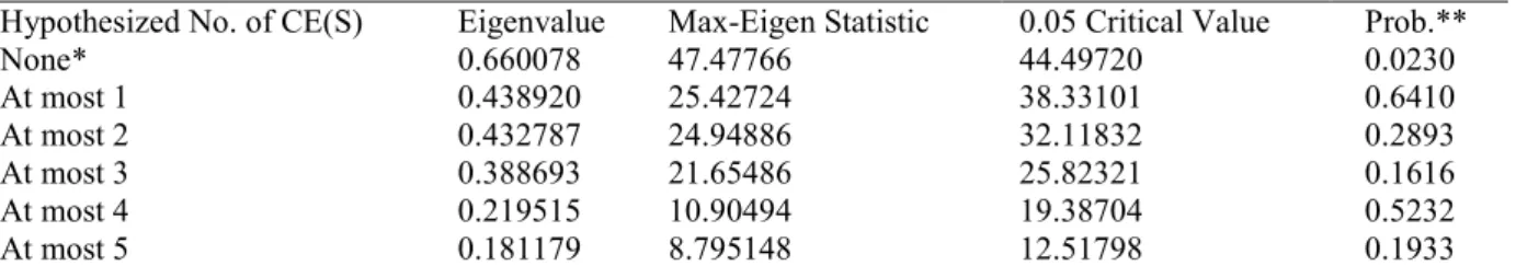
Table 4. Johansen Unrestricted Cointegration Rank Test (Maximum Eigenvalue) Result; Series: LMD, LRGDP, LRIR, LFIR, LINF, LEXR
Hypothesized No. of CE(S) Eigenvalue Max-Eigen Statistic 0.05 Critical Value Prob.**
None* 0.660078 47.47766 44.49720 0.0230 At most 1 0.438920 25.42724 38.33101 0.6410 At most 2 0.432787 24.94886 32.11832 0.2893 At most 3 0.388693 21.65486 25.82321 0.1616 At most 4 0.219515 10.90494 19.38704 0.5232 At most 5 0.181179 8.795148 12.51798 0.1933
Max-eigenvalue test indicates 1 cointegrating eqn(s) at the 0.05 level *denotes rejection of the hypothesis at the 0.05 level
**Mackinno-Haug-Michelis (1999) p-values. Source: Authors’ computation from Eviews 8.0.
4.3 Error Correction Test Result
Error Correction Mechanism (ECM) was used to determine the speed of adjustment of the disequilibrium conditions in the estimated time series. The result is presented in Table 5.
Table 5. EC Test Result (at 5per cent significance level)
Variable Coefficient S.E T-statistic Prob. Constant 0.091405 0.100833 0.906494 0.3702 D(LGDP) -0.012124 0.190277 -0.063717 0.9495 D(LINT) 0.099430 0.469038 0.211986 0.8332 D(LFIR) -0.325483 0.199123 -1.634582 0.1102 D(LINF) -1.061148 0.129603 -8.187686 0.0000 D(LEXR) -0.230044 0.275364 -0.835417 0.4086 EC(-1) -0.223089 0.103365 -2.158268 0.0371 Source:Authors’ computation from Eviews 8.0.
The result presented in Table 5 shows that, at 5 per cent significance level, the EC variable indicate a negative signed coefficient of -0.223089. This means that about 22 per cent of disequilibrium conditions in the model is corrected within the first quarter.
4.4 Regression Results
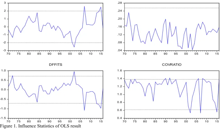
The specified model for this study was first estimated using Ordinary Least Square (OLS) technique. The result presented in the Appendix shows that real income (RGDP) was not significant, and D.W statistic indicated serial correlation since it was less than R-squared. However, out of the 46 observations used in the study, some of the values were identified to be unusual or substantially different from the bulk of the data (outliers). This might result from mistake in data entering, such as adding extra zeros to a number or misplacing a decimal point (Wooldridge, 2009) We confirmed this finding by looking at the influence statistics and leverages for the estimated equation. The Influence Statistics of the OLS result are displayed in Figure 1.
-3 -2 -1 0 1 2 3 70 75 80 85 90 95 00 05 10 15 RStudent .04 .08 .12 .16 .20 .24 .28 70 75 80 85 90 95 00 05 10 15 Hat Matrix -1.5 -1.0 -0.5 0.0 0.5 1.0 70 75 80 85 90 95 00 05 10 15 DFFITS 0.4 0.6 0.8 1.0 1.2 1.4 1.6 70 75 80 85 90 95 00 05 10 15 COVRATIO Influence Statistics
Figure 1. Influence Statistics of OLS result Source: Authors’ computation from Eviews 8.0.
However, the spikes in the graphs for all five influence measures point to observation 33 as being an outlier. This finding is confirmed by the leverage plot view of the OLS regression result.
-3 -2 -1 0 1 2 3 -1 .5 -1 .0 -0.5 0 .0 0.5 1.0 1 .5 LRGDP -3 -2 -1 0 1 2 3 -.6 -.4 -.2 .0 .2 .4 .6 .8 LINT -2 -1 0 1 2 3 -1 .5 -1 .0 -0.5 0 .0 0.5 1.0 1 .5 LFIR -3 -2 -1 0 1 2 3 -1 .5 -1 .0 -0.5 0 .0 0.5 1.0 1 .5 LINF -3 -2 -1 0 1 2 3 -2 -1 0 1 2 LEXR
LMD vs Variables (Partialled on Regressors)
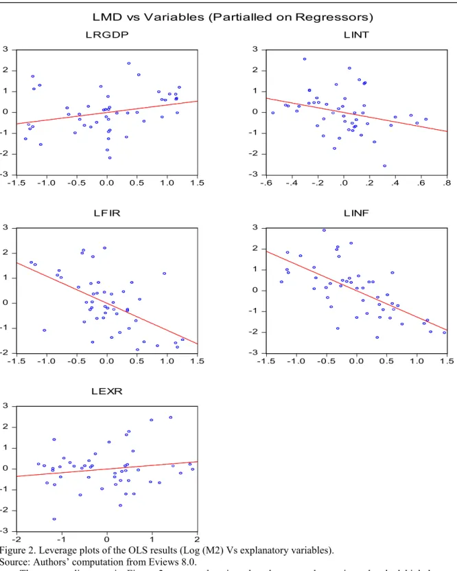
Figure 2.Leverage plots of the OLS results (Log (M2) Vs explanatory variables). Source:Authors’ computation from Eviews 8.0.
The scatter diagrams in Figure 2 support the view that there are observations that had high leverage, especially in the relationship between M2 and the explanatory variables.
4.5 Robust Linear Regression Result from MM-Estimation
Given the presence of outliers as seen above, we re-estimated the regression using robust MM-Estimation. The estimation output is displayed in Table 6.
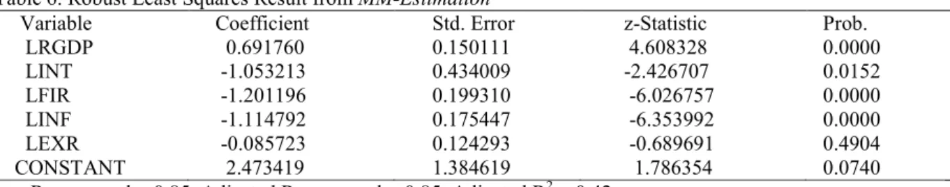
Table 6. Robust Least Squares Result from MM-Estimation
Variable Coefficient Std. Error z-Statistic Prob. LRGDP 0.691760 0.150111 4.608328 0.0000 LINT -1.053213 0.434009 -2.426707 0.0152 LFIR -1.201196 0.199310 -6.026757 0.0000 LINF -1.114792 0.175447 -6.353992 0.0000 LEXR -0.085723 0.124293 -0.689691 0.4904 CONSTANT 2.473419 1.384619 1.786354 0.0740 Rw-squared = 0.85, Adjusted Rw-squared = 0.85, Adjusted R2 = 0.42,
Rn-squared statistic = 161.3116, Prob (Rn-squared stat.) = 0.000000 Source: Authors’ computation from Eviews 8.0.
Turning to the coefficient estimates, we see the effect on the coefficient estimates of moving from least squares to robust MM-Estimation. Based on the result presented in Table 6, real income is statistically significant and positively related with real demand for money. The result provides some support for the monetarists’ theoretical proposition that there exists a direct link between the M2 money stock and money income. Moreover, the long-run income elasticity estimate is found to be greater than zero (0.69). The result implies that, when there is 1 per cent increase in real income of people, their demand for real balance will increase by 69per cent. On the other hand, real interest rate is statistically significant and inversely related to real demand for money. Considering the coefficients, if CBN raises interest rate by 1 per cent, demand for money by individuals will decrease by about 105 per cent. Consequently, foreign interest rate is statistically significant and the coefficient indicates negative relationship with real money demand in Nigeria.
This finding shows the negative impact of foreign currency; especially the U.S dollar on the demand for real balances in Nigeria. The economic implication is that as U.S interest rate increases by 1per cent, it will lead to depreciation of the naira demanded by 120 per cent. The result also indicated inflation as a significant determinant of demand for money. This means that with 1 per cent increase in inflation rate, it will discourage people from holding cash balance by almost 111 per cent. The economic implication is that; people will prefer to hold alternative assets instead since money has lost its purchasing power. On the contrary, real exchange rate turned out to be a weak or insignificant determinant but displayed exertion of positive influence on money demand during the period under review. However, despite the fact that exchange rate is found to be a weak determinant of money demand, the economic implication is that if the exchange rate is increased by 1 per cent, Nigerians that engage in international trade will increase their demand for local currency, i.e., naira to exchange for foreign currencies especially U.S dollar by 8.5 per cent.
The bottom portion of the output displays the R2 and R2w goodness-of-fit and adjusted measures, along which indicate that the model accounts for roughly 42-85 per cent of the variation in the constant-only model. The statistic of 161.31corresponding to p-value of 0.000 indicates strong rejection of the null hypothesis that all non-intercept coefficients are equal to zero. The z-statistics in the output are based on Huber Type I covariance estimates.
4.6 Stability Test Results
The stability test results are plotted in Figures 3 and 4.
-20 -10 0 10 20 30 1980 1985 1990 1995 2000 2005 2010 2015
CUS UM 5% S ignific ance
Figures 3. CUSUM test for the M2 regression Source: Authors’ result from Eviews 8.0.
The CUSUM stability test result displayed in Figure 3 shows that money demand function was unstable for the entire period under consideration. This is because at 5 per cent significance level, the statistic does not
completely lie within the pairs of line known as critical region, especially from 2014 to 2016. This finding is contrary to the results obtained by Nigerian studies such as Sanya (2013), Sanya and Awe (2014), Nduka et al. (2013), Okonkwo et al. (2014), Imimole and Uniamikogbo (2014), Doguwa et al. (2014), Aiyedogbon et al.
(2013), Nduka (2014) and El-Rasheed et al. (2017).
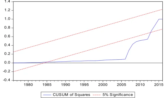
Similarly, the plot of the cumulative sum of squares (CUSUMSQ) of the recursive residuals in Figure 4.4, indicate that, real money demand function was not completely stable during the study period. This is because at 5 per cent significance level, the CUSUMSQ statistic does not completely lie within the critical region.
-0.4 -0.2 0.0 0.2 0.4 0.6 0.8 1.0 1.2 1.4 1980 1985 1990 1995 2000 2005 2010 2015 CUSUM of Squares 5% Significance
Figure 4. CUSUMSQ test for the M2 regression Source: Authors’ result from Eview 8.0.
The result showed that there was deviation from 1985 to 2013 before returning to stability from 2014 to 2016. Similar result was obtained by Nduka (2014) but contrary to the submissions of all other previous studies in Nigeria.
4.7 Structural Breakpoint Test Result
The Multiple Breakpoints test (Bai-Perron tests of L+1 vs. L globally determined breaks) results are shown in Table 7.
Table 7: Multiple breakpoints test results
Break Order Break date
1 1978 2 1979 3 1986 4 1987 5 1995 6 1999 7 2002 8 2007 9 2008
Source:Authors’ Result from Eview 8.0.
Multiple breakpoint test result displayed in Table 7 reveal moments of structural breaks in 1978, 1979, 1986, 1987, 1995, 1999, 2002, 2007 and 2008. In Nigerian studies, Omotor, (2011) had earlier reported break dates in 1981, 1992 and 1994, while Chukwu et al. (2010) also found evidence of structural break in 1994, 1996 and 1997. Kumar et al. (2010) also found cases of structural breaks in 1986 and 1992, while Nduka (2014) reported break date in 2005.
5. Conclusion
This paper empirically examined real money demand function and its stability in Nigeria using annual time series data from 1970 to 2016 inclusive.In the light of the findings of this study, money demand in Nigeria is strongly determined by real income, interest rate, inflation rate, and foreign interest rate. This implies that, CBN can make efficient use of these variables to control inflation in order to stabilize money demand to match money
supply in Nigeria. Consequently, the findings revealed an unstable money demand function in Nigeria with 9 structural breaks recorded during period under review.
However, based on the findings of the paper, it would not have been out of place if CBN effectively managed interest rate, inflation and exchange rate as instruments of monetary policy to ensure stable demand for real money balances in Nigeria during the period. Also, this would have helped the apex bank to avoid undesired structural breaks recorded. Furthermore, unprecedented financial innovations and other institutional reforms that took place in the financial sector and shocks that bedeviled the economy during the period might have also contributed to the instability of the money demand function. The structural break dates recorded are consistent with the impact of major economic events that took place within the scope of the study. These include; fall in oil revenue before and after the introduction of Structural Adjustment Programme (SAP) in 1986 which generated chains of economic problems in Nigeria. The breaks at some point could also be due to the impact of 2004 bank consolidation policy of CBN and global financial crisis that affected many economies which became more pronounced in 2008.
Based on the findings of the study, the following are recommended for policy options: i. CBN should target broad money aggregates to control inflation in Nigeria;
ii. In order to stabilize money demand in Nigeria, CBN should conduct monetary policy regime that focuses on stabilizing the real macroeconomic environment; and
iii. CBN should conduct monetary policy regime that aligns with fiscal policy to accommodate exogenous shocks to the economy that could lead to incidence of undesired structural breaks.
References
Abdullah, M.; Chani, M. I. & Ali, A. (2013). Determinants of money demand in Pakistan: Disaggregated expenditure approach. World Applied Science Journal, 24(6), 765-771. DOI: 10.5829/idosi.wasj.2013.24.06.1227.
Ahad, M. (2015). Financial development and money demand function: Cointegration, causality and variance decomposition analysis for Pakistan, Munich Personal RePEc Archive (MPRRA) Paper No. 70033, Retrieved from https://mpra.ub.uni-uenchen.de/70033/.
Aiyedogbon, J. O., Ibeh, S. E., Edefe, M. & Ohwofasa, B. O. (2013). Empirical analysis of money demand function in Nigeria. International Journal of Humanitarian and Social Sciences, 3(8), 132-147. Retrieved from http//:www.ijhssnet.com.
Ajayi, S. I. (1974). The demand for money in Nigerian economy: Comments and extension. Journal of Economics and Social Studies, 16(1), 165-174.
Ajayi, S. I. (1977). Some empirical evidences on demand for money in Nigeria. American Economists, 21(1), 51-54.
Akinlo. A. E. (2006). The stability of money demand in Nigeria: An autoregressive distributed lag approach.
Journal of Policy Modeling, 28, 445-452.
Apere, T. O. & Karimo, T. M. (2014). The demand for real money balances in Nigeria: Evidence from a Partial Adjustment Model. European Journal of Business Economics and Accountancy, 2(2), 1-14.
Arinze, A. C., Darrat, A. F & Meyer, D. J. (1990). Capital mobility, monetization, and money demand: Evidence from Africa. Centre for Economic Research on Africa, School of Business, Montclair State University Upper Montclair, New Jersey, 1-14.
Azim, P., Ahmed, N., Ullah, S. Bedi-uz-Zaman, & Zakaria, M. (2010). Demand for money in Pakistan: An ARDL Approach. Global Journal of Management and Business Research, 9(10), 76-80
Baba, I., Kenneth, O. B. & Williams, O. (2013). A dynamic analysis of the demand for money in Ghana. African Journal of Social Sciences, 3(2), 19-29.
Bahmani-Oskooee, M. & Bohl, M. (2000). Monetary unification and the stability of the German nm3 money demand function. Economics Letters, 66, 203–208.
Bahmani-Oskooee, M. & Chomsisengphet, S. (2002). Stability of M2 money demand function in industrial
countries. Applied Economics, 34, 2075-2083.
http://www.tanfonline.com/doi/abs/10.1080/00036840210128744.
Bahmani-Oskooee, M. & Sungwon, S. (2006). Stability of the demand for money in Korea. International Economic Journal, 18(2):85-95.
Bai, J. & Perron, P. (2003). Computing and analyzing of multiple structural change models. Journal of Applied Econometrics, 18(1), 1-22.
Ball, L. (2001). Another look at long-run money demand. Journal of Monetary Economics, 47, 31-44. http://dx.doi.org/10.1016/S0304-3932(00)00043-X.
Bitrus, Y. P. (2011). Demand for money in Nigeria. European Journal of Business and Management, 3(6), 63-85. Brown, R., Durbin, J. & Evans, J. (1975). Techniques for testing the constancy of regression relationships over
Busari, D. T. (2006). On the stability of demand for money function in Nigeria. Journal of Economic and Financial Review, 42(3), 49-68.
Central Bank of Nigeria (2016). Statistical bulletin. Retrieved from www.cenbank.org
Choi, K. & Jung, C. ((2009). Structural changes and the US money demand function. Applied Economics, 41, 1251-1257. http://dx.doi.org/10.1080/00036840601007385.
Choi, K. & Jung, C. (2011). Structural Changes and the US money demand function. Journal of Applied Economics (published online), 18(2):1251-1257. https://doi.org/10.1080/00036840601007385.
Chukwu, J. O., Agu, C. C. & Onah, F. E. (2010). Co-integration and structural breaks in Nigerian long-run money demand function. International Research Journal of Finance and Economics, 38.
Dagher, J. & Koven, A. (2011). On the stability of money demand in Ghana: A bound testing approach.
International Monetary Fund, WP/11/273.
Deadman, D. & Ghatak, S. (1981). On the stability of the demand for money in India. Indian Economic Journal, 29, 41-54.
Doguwa, S. I.; Olowofeso, O. E.; Uyaebo, S. O. U.; Adamu, I. & Bada, A. S. (2014). Structural breaks, co-integration and demand for money in Nigeria. CBN Journal of Applied Statistics, 5(1), 15-33.
Edet, B. N., Udo, S. U. & Etim, O. U. (2017). Modeling the demand for money function in Nigeria: Is there Stability? Bulletin of Business and Economics, 6(1), 45-57.
El-Rasheed, S., Addullah, H., & Dahalan, J. (2017). Monetary uncertainty and demand for money stability in Nigeria. an autoregressive distributed lag approach. International Journal of Economics and Financial Issues, 7(1), 601-607.
Ewing, B. T. & Payne, J. E. (1998). Some recent international evidence on the demand for money. Studies in Economics and Finance, 19, 84-107. https://doi.org/10.1108/eb028754.
Farazmand, H.; Ansari, M. S. & Moradi, M. (2016). What determines money demand? Evidence from MENA.
Economic Review, 45,151-169, July.
Folarin, O. E. & Asongu, S. A. (2017). Financial liberalization and long-run stability of money demand in Nigeria. African Governance and Development Institute Working Paper WP/17/018
Hamdi, H. Said, A. & Sbia, R. (2015). Empirical evidence on the long-run money demand function in the Gulf Cooperation Council Countries. International Journal of Economics and Financial Issues, 5(2), 603-612. Hoffman, D. L. & Rasche, R. H. (2001). Money demand in U.S. and Japan: Analysis of stability and the
importance of transitory and permanent shocks. Retrieved from http://ideas.repec.org/e/pra180.html. Hounsou, R. (2017). Analysis of the determinants of the demand for money in the Franc Zone: A study of panel
data, American Based Research Journal, February. Retrieved from https://ssrn.com/abstract=2935533). Ighadaro, C. A. U. & Ihaza, I. M. (2008). A co-integration and error correction approach to broad money
demand in Nigeria. Journal of Research in National Development, 6(1), 12-21.
Imimole, B. & Uniakomikogbo, S. O. (2014). Testing for the stability of money demand function in Nigeria.
Journal of Economic and Sustainable Development, 5(6), 123-130.
Inoue, T. & Hamori, S. (2008). An empirical analysis of the money demand function in India. Institute of Developing Economies, India.
International Monetary Fund (2016). International Global Financial Statistics. Retrieved from www.imf.org/ifs Iyoboyi, M. & Pedro, L. M. (2013). The demand for money in Nigeria: Evidence from bounds testing approach.
Business and Economics Journal, 76, 1-11.
Johansen, S. (1988). Statistical analysis of cointegrated vectors. Journal of Economic Dynamics and Control, 12(203), 231-254. http://doi.org/10.1016/0165-1889(88)90041-3.
Jung, A. (2016). A portfolio demand approach for broad money in the euro area. European Central Bank (ECB) Working Paper No 1929, July. Retrieved from www.ecb.europa.eu).
Kiptui, M. C. (2014). some empirical evidence on the stability of money demand in Kenya, International Journal of Economics and Financial Issues, 4(4), 849-858.
Kjosevski, J. (2013). The determinants and stability of money demand in the Republic of Macedonia. Zb. Rad. Ekon. Fak. Rij., 31(1), 35-54.
Kones, A. (2014). Impact of monetary uncertainty and economic uncertainty on demand for money in Africa. (Unpublished Doctoral Thesis). University of Wisconsin. Retrieved from http://dc.uwm.edu.etd.
Kumar, S. (2013). Australasian money demand stability: Application of structural break tests. Applied Economics, 45(8), 1011-1025. http://dx.doi.org/10.1080/00036846.2011.613788.
Kumar, S., Fargher, S. & Don, J. W. (2010). Money demand stability: A case study of Nigeria, Auckland University of Technology, Auckland, New Zealand. Retrieved from https://mpra.ub.un-muenchen.de/id/eprint/26074.
Mall, S. (2013). Estimating a function of real demand for money in Pakistan: An application bound testing approach to co-integration. International Journal of Computer Applications, 79(5), 37-50.
on the demand for money in Nigeria. International Journal of Finance and Economics, 3(58), 73-88. Nagayasu, J. (2003). A re-examination of the Japanese money demand function and structural shifts. Journal of
Policy Modeling, 25, 359-375. http://www.sciencedirect.com/science/article/pii/S0161-8938(03)00010-3. Nduka, E. K, Chukwu, J. O. & Nwakaire, O. N. (2013). Stability of demand for money in Nigeria. Asian Journal
of Business and Economics, 3(34), 1-8.
Nduka, E. K. (2014). Structural breaks and the long run stability of demand for broad money function in Nigeria: A Gregory-Hanson Approach. Economics and Finance Letters, 1(8), 76-89.
Nyong, M. O. (2014). The demand for money, structural breaks and monetary policy in the Gambia. Developing Country Studies, 4(19), 93-106.
Odama, J. S. (1974). The demand for money in the Nigerian economy: A comment, Nigerian Journal of Economics and Social Studies, 16(1), 175-178.
Ogbonna, B. C. (2015). Exchange rate and demand for money in Nigeria. Macrothink Institute Research in Applied Economics, 7(2), 21-37. http://dx.doi.org/10.5296/rae.v7i.7919.
Ojo, O. (1974). The demand for money in Nigerian economy: Some comments. Nigeria Journal of Economic and Social Studies, 16(1), 149-152.
Okonkwo, O. N., Ajudua, E. I. & Alozie, S.T. (2014). Empirical analysis of money demand stability in Nigeria.
Journal of Economics and Sustainable Development, 5(14), 138-145.
Omotor, D. G. & Omotor, P. E. (2011). Structural breaks, demand for money and monetary policy in Nigeria.
EKONOMSKI PREGLED, 62(9-10), 559-582.
Onafowora, O. A. & Owoye, O. (2011). Structural adjustment and the stability of the Nigerian money demand function. International Business & Economic Research Journal, 3(8). https://doi.org/10.19030/iber.v3i8.3714.
Sanya, O. & Awe, A. A. (2014). Impact of Commodity Price Fluctuations on the Stability of Nigerian Money Demand Function. International Journal of Arts and Commerce, 2(7), 25-42.
Sanya, O. (2013). Impact of financial liberalization on the stability of Nigerian money demand function.
International Journal of Economics, Business and Finance, 2(1), 1-8.
Sarwar, H. Sarwar, M. & Waqas, M. (2013). Stability of money demand function in Pakistan. Economic and Business Review, 15(3), 197-212.
Suliman, S. Z. & Dafaalla, H. A. (2011). An econometric analysis of money demand function in Sudan, 1960 to 2010. Journal of Economics and International Finance, 3(16), 793-800.
Taiwo, M. (2012). The implication of effectiveness of demand for money on economic growth. ACTA Universitatis Danubius, 8(1), 34-48.
Teriba, O. (1974). The demand for money in the Nigerian economy: Some methodological issues and further evidence. Nigerian Journal of Economics and Social Studies, 16(3), 153-163.
Tomori, S. (1972). The demand for money in the Nigerian economy. Nigerian Journal of Economics and Social Studies, 16(1), 179-187.
Tümtürk, O. (2017). Stability of money demand function in Turkey. Business and Economics Research Journal, 8(1),35-48. DOI Number: 10.20409/berj.2017126243.
Wooldridge, J. M. (2009). Introductory econometrics: A modern approach. Fourth edition. Australia: South Western Cengage Learning.