Computational Bayesian techniques applied to cosmology

(1)

Computational Bayesian techniques

applied to cosmology

Sonke Hee

Churchill College

2017 April

(2)

(3)

Summary

This thesis presents work around 3 themes: dark energy, gravitational waves and Bayesian inference. Both dark energy and gravitational wave physics are not yet well constrained. They present interesting challenges for Bayesian inference, which attempts to quantify our knowledge of the universe given our astrophysical data.

A dark energy equation of state reconstruction analysis finds that the data favours the vacuum dark energy equation of state w = −1 model. Deviations from vacuum dark energy are shown to favour the super-negative ‘phantom’ dark energy regime ofw < −1, but at low statistical significance. The constraining power of various datasets is quantified, finding that data constraints peak around redshiftz =0.2 due to baryonic acoustic oscillation and supernovae data constraints, whilst cosmic microwave background radiation and Lyman-αforest constraints are less significant. Specific models with a conformal time symmetry in the Friedmann equation and with an additional dark energy component are tested and shown to be competitive to the vacuum dark energy model by Bayesian model selection analysis: that they are not ruled out is believed to be largely due to poor data quality for deciding between existing models.

Recent detections of gravitational waves by the LIGO collaboration enable the first grav-itational wave tests of general relativity. An existing test in the literature is used and sped up significantly by a novel method developed in this thesis. The test computes posterior odds ratios, and the new method is shown to compute these accurately and efficiently. Compared to computing evidences, the method presented provides an approximate 100 times reduction in the number of likelihood calculations required to compute evidences at a given accuracy. Further testing may identify a significant advance in Bayesian model selection using nested sampling, as the method is completely general and straightforward to implement. We note that efficiency gains are not guaranteed and may be problem specific: further research is needed.

(4)

(5)

Declaration

This dissertation is the result of my own work and includes nothing which is the outcome of work done in collaboration except as declared in the Preface and specified in the text.

It is not substantially the same as any that I have submitted, or, is being concurrently submitted for a degree or diploma or other qualification at the University of Cambridge or any other University or similar institution except as declared in the Preface and specified in the text. I further state that no substantial part of my dissertation has already been submitted, or, is being concurrently submitted for any such degree, diploma or other qualification at the University of Cambridge or any other University or similar institution except as declared in the Preface and specified in the text

It does not exceed the prescribed word limit (60,000 words) for the relevant Degree Com-mittee.

(8)

(9)

Acknowledgements

Without my supervisors, Mike Hobson and Anthony Lasenby (as well as Will Handley who was an additional de facto supervisor throughout the years), this thesis would be considerably emptier if not blank. Thank you for the direction and genius that guided the research and overcame all problems.

The work in this dissertation has substantially benefited from a steady stream of discussion with (mostly forced upon) a variety of brilliant researchers within the IoA and MRAO groups. Thanks to Farhan Feroz for initial help with using MultiNest, Jose Vázquez for sharing various codes for reference, Ed Higson for disseminating a masterful understanding of errors in nested sampling, and Alvin Chua for supervisorial guidance on gravitational wave astronomy. With immeasurable thanks to Karen Scrivener for looking after everyone in MRAO so well.

My motivation over three and a half years of research has been greatly aided by a fantastic office environment. I am grateful to Richard Wolstenhulme for a consistent and holistic work efficiency programme, to Will Handley for being the office oracle on all matters physics and Linux, Do Young Kim for being positively lovely all of the time, and Carina Negreanu for always being a great source of constructive criticism and fun discussions. The K34 office will be greatly missed.

There is much to be said for the ‘Cambridge experience’, and I am very grateful for the constant support offered and opportunities for personal growth provided. Churchill College has been central to both welfare and development, and I am especially grateful to Rebecca Sawalmeh and Shelley Surtees for making Churchill College such a welcoming place. I am also grateful for all the time, effort and wisdom that the Møller centre coaches have offered whilst I was fortunate enough to be involved in their training program.

Finally, the warmest gratitude goes to my family for getting me to where I am: immeasurable thanks to Anja Hee, Anissa Hee, Stephen Tucker and Cedrik Hee - you all know what you have done. Especially, thank you mum for the financial and moral support. I dedicate this thesis to Aira, Anne, and a plum-sized 3 month old baby undergoing a phase of accelerated expansion.

(10)

(11)

Chapter

1

Outline

Although every generation of PhD student must think this, we are at a remarkable time to be studying cosmology. We are privileged to have a wealth of observations that constrain models of the universe, from large scale structure surveys that analyse the universe’s recent evolution to a clear image of the cosmic microwave background radiation that shows a snapshot of the universe’s distant past. Alongside rapid development in cosmological data precision, the Bayesian statistical framework to analyse this data has developed: as an example, the remarkable contribution nested sampling has made to the field of Bayesian model selection.

In order to fit observations, cosmological models posit the existence of dark energy. Dark energy refers to a hypothetical repulsive force that is required to explain observations of the recent accelerated expansion of the universe. Dark energy is poorly understood despite its dominant contribution to the current universe’s evolution. This thesis constrains dark energy behaviour phenomenologically using data-driven analysis techniques. It also presents a novel method of quantifying the various dataset contributions to such phenomenological constraints. Additionally a specific dark energy model extension is tested and shown to be competitive to the standard dark energy description, though the new model’s competitiveness stems from a lack of data with which to constrain the models. Several of the analysis techniques can and have been applied to other areas of cosmology. The methods provide useful tools for future research as new observational missions provide ever more powerful data.

A new type of observation has become available in 2016 with the first direct detection of gravitational waves by the advanced LIGO detectors. Future missions are being upgraded and developed, including further ground based observatories as well as space based gravitational

(12)

2 Chapter 1. Outline

wave observatories. These missions will detect gravitational waves more clearly as well as at different frequencies. The first detection was heralded as the dawning of gravitational wave astronomy, and the future is rich with possibility regarding its application. A particularly interesting application is in testing general relativity in the strong field regime. This thesis expands on the use of gravitational waves to test general relativity by using a novel method to improve the accuracy of the Bayesian model selection calculations. The method was first developed for the aforementioned dark energy investigation and is generally applicable to any Bayesian model selection problem.

The thesis presents both cosmological results for understanding dark energy and the future potential of gravitational wave tests of general relativity. Alongside these are a heavy emphasis on the analysis techniques developed. Below is a more detailed overview of each chapter and their relation to the thesis generally.

1.1

Chapter synopsis

Chapter2presents an overview of the dark energy and gravitational wave physics used through-out the thesis. Specifically, section 2.1 describes the Einstein field equations of general re-lativity and how to obtain the standard cosmological model from these. A quick overview of the universe’s evolution history is presented to frame the uniqueness of the dark energy era we find ourselves in. Observations to constrain our universe are described, including the cosmic microwave power spectrum, baryonic acoustic oscillation measurements and supernovae meas-urements. Section2.2reviews the vacuum energy interpretation of the cosmological constant which forms the ‘Λ’ part of the ΛCDM model. Alternate dark energy models are reviewed briefly to highlight how constraining the dark energy equation of state parameter can shape our understanding of permissible dark energy models. Section2.3reviews the gravitational wave equations, wave detections and tests of general relativity.

Chapter3reviews the Bayesian inference framework which underpins our ability to constrain cosmological models with data. The thesis is inherently Bayesian throughout, and time is dedicated to define parameter estimation and model selection. Section3.2describes the nested sampling algorithm which is used to compute parameter estimates and the model selection variables. Computational implementations (most notably PolyChord) are discussed, with an emphasis on their robustness and the errors computed on the quantities of interest for inference. Further discussions on applying this framework to cosmological investigations and the gravitational wave problem are presented.

Chapter4presents and verifies a new method developed in this thesis for calculating model selection quantities (posterior odds ratios and Bayes factors). Traditionally, these quantities are

(13)

1.1. Chapter synopsis ₃

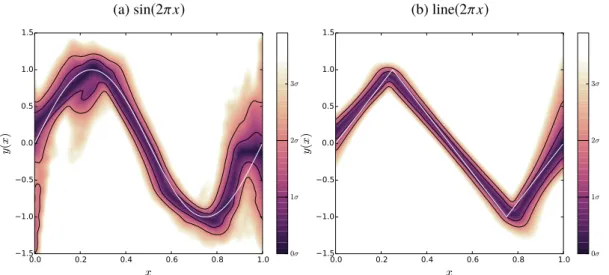
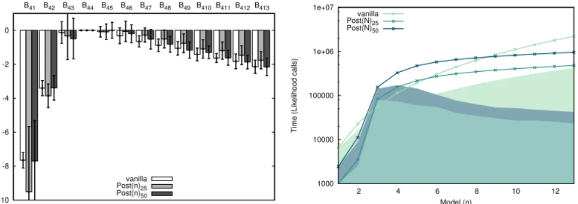
difficult to obtain, with nested sampling providing the best method by computing ‘evidences’ for each model from which model selection is trivial. The new method avoids the expensive evidence calculation altogether and instead uses parameter estimation on a model selection hyper-parameter to obtain posterior odds ratios. The method is verified on a toy model and then applied to a phenomenological investigation of potentially time varying dark energy equation of state behaviour. The new method is shown to compute Bayes factors reliably when the traditional evidence calculations are not reliable.

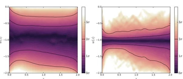
Chapter5expands on the phenomenological dark energy investigation by investigating more fully the dependence of dark energy behaviour on the choice of datasets. A novel formalism of the Kullback-Leibler divergence is presented, where the Kullback-Leibler divergence is used to define the information addition when moving from prior to posterior parameter distributions (where the additional information is due to the datasets used). The novel formalism identifies the equation of state constraining power of the datasets as a function of time. The results show that

ΛCDM is consistent with all potential time varying behaviour. Additionally, we observe that baryonic acoustic oscillations and supernovae data provide the strongest constraints in general, whilst Lyman-αbaryonic acoustic oscillation measurements provide much needed additional constraining power at earlier times.

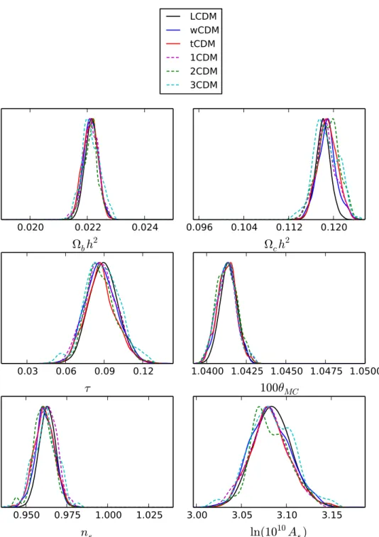
Chapter6continues to investigate the dark energy equation of state behaviour but from an alternative model perspective (rather than chapters4and5which present model-independent investigations). A model is presented where an additional matter density component is intro-duced with equation of state w = −2/3. The introduction is justified by a symmetry in the evolution history of the universe (in terms of conformal time). The model is not disfavoured compared to ΛCDM in a Bayesian model selection analysis, but the new model parameter estimates are consistent with ΛCDM. An additional model is tested as a natural extension in which the additional matter component’s equation of state is allowed to vary, again showing no preference for or againstΛCDM.

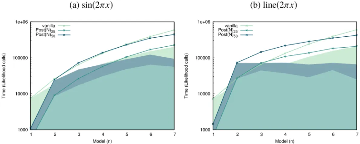
Chapter7utilises the novel method described in chapter4 to improve the efficiency of a gravitational wave test of general relativity. The test is a model-independent phenomenological test of deviations from general relativity in the phase coefficients of the gravitational wave. Similar tests have been used by the LIGO collaboration to find that the observed gravitational waves show no sign of deviations from general relativity. The new method is able to compute Bayes factors significantly faster than when computing evidences first. For a toy sinusoidal model with a wave signal without deviations, the new method computes equivalently accurate posterior odds ratios with 24 times less computational resource (fewer likelihood calculations). This efficiency gain is also observed using a more physically relevant model: gravitational waves produced by Kerr model binary coalescence. For a mock data injection without deviation from

(14)

4 Chapter 1. Outline

general relativity, the efficiency gain is on order ≈ 100, though the analysis could not be completed as thoroughly as for the toy model due to general computational limitations.

Chapter8summarises the key results and discusses future applications. The four chapters of original work present primarily advancements in dark energy and gravitational wave data analysis. The new method for computing posterior odds ratios is applicable more widely to any model selection problem. The novel formalism of the Kullback-Leibler divergence is also applicable more generally to any function that is constrained by data, and has already been adopted by other authors. We conclude that generally the data analysis techniques are of interest widely in the astrophysical community as well as outside of it once the adoption of nested sampling prevails beyond the astrophysics community.

(15)

Chapter

2

Cosmological and gravitational

framework

In this chapter we present the theoretical framework used throughout this thesis. The mathem-atical arena for this work is general relativity. We start with the Einstein field equations and move on quickly to cosmological and wave solutions. Specifically, we present the standard model of our universe, how to extend to alternate dark energy models, and the gravitational wave equations. The most detail is dedicated to testable observations within these topics as that is the focus of this thesis: data-driven model analysis to constrain dark energy physics and improving data-driven gravitational wave tests of general relativity.

In section2.1 we present the textbook ΛCDM cosmological model of the universe, ob-tained by solving the Einstein field equations using thecosmological principle, and outline the dynamical behaviour of this model and how it can be tested by astrophysical observations. In section2.2, extensions to the dark energy component of this model are analysed. Finally, sec-tion2.3presents the gravitational wave solutions to the Einstein field equations and describes the promising field of gravitational wave astronomy.

This short review uses a wide range of materials, with citations introduced as needed, whilst using as references the textbooks ofDodelson(2003) andHobson et al.(2006) and also the very clear introductory chapters in the theses ofVázquez(2013),Handley(2016) andChua(2017).

(16)

6 Chapter 2. Cosmological and gravitational framework

2.1

The concordance model:

Λ

CDM

Over the years many cosmological models have been proposed, from Einstein’s attempt at creating a static universe to ones containing only matter and radiation. At present the consensus is that the ΛCDM model fits all cosmological observations remarkably well. The building blocks of the universe that are familiar to us, namely ordinary (baryonic) matter and photons (radiation), only account for about 5% of this proposed model. It should seem odd to anyone that we believe a model where 95% of its contents are hitherto unknown to us, but cosmologists have been led to this conclusion by a host of interesting astrophysical observations.

In this section we outline what theΛCDM model is and to discuss observational data relating to cosmology. We assume a basic knowledge of general relativity but do not rely on it heavily in this introduction as the thesis focusses on data analysis rather than theory; an understanding of spacetime, the related 4-vectors and tensors, and notational index raising and lowering would help but are not necessary to understand the principles.

2.1.1 Einstein field equations and cosmological solutions

John Wheeler famously remarked that “spacetime tells matter how to move; matter tells space-time how to curve”. This direct relation between matter and spacespace-time curvature is captured even more succinctly by the Einstein field equationsa:

Gµν =κTµν (2.1)

where Gµνis the Einstein tensor representing the curvature of spacetime and Tµν is the energy-momentum tensor representing the matter and energy content. κ=8πG/c4 is a constant which can easily be derived from approximation to the Newtonian gravitational field equations; it is composed of Newton’s gravitational constant G, speed of lightc, as well asπb. The subscripts

µandνhide the complexity of the gravitational field equations. These subscripts (or indices) run from 0 to 3 to define ‘tensors’ in differential geometry, whereµ=0 are time coordinates and the rest are spatial. After symmetry considerations, equation (2.1) comprises 6 independent non-linear 2nd order partial differential equations, with solutions only possible by making assumptions about the matter and energy distribution or geometry of the spacetime.

To solve equation (2.1) for a model of our universe we will therefore make an assumption about its matter and energy distribution: the universe is homogeneous when viewed on suffi-ciently large scales. This particular assumption is known as the cosmological principleand, although impossible to confirm for the whole universe based on our limited singular vantage

a_{Omitting the cosmological constant for now.}

(17)

2.1. The concordance model: ΛCDM ₇

point on Earth, it seems empirically justified: galaxy surveys suggest that our local universe matter distribution is homogeneous at a length scale of 63.3±0.7h−1Mpcc(Ntelis et al. 2017) (whereh≈0.7 is suggested by theΛCDM model).d

We use the cosmological principle to create a maximally symmetric spatial component in the geometry. Choosing comoving coordinates so that an observer with constant spatial coordinates would observe this isotropic universe (amongst other conveniences; such observers are referred to as ‘fundamental observers’), one can obtain the Friedmann-Lemaître-Robertson-Walker (FLRW, or often FRW) metric:

ds2= _dt2₋_a₍_t₎2 dχ2+_S2₍χ)_dΩ2_, (2.2) whereS2(χ)=            sin2(χ) ;k =1, χ2 _;_k =₀, sinh2(χ) ;k =−1. (2.3)

The metric above describes a spacetime with a simple time coordinate and a spatial component

a(t)2

dχ2+_S2₍χ)_dΩ2_{. The spatial component is constant in time aside from the aptly named}

scale factor a(t). The geometry of the spatial component is described by the functionS2(χ) as open, flat or closed, depending on the curvature parameter k. Additionally, dΩ2=dθ2 + sin2(φ)dφ2 is the solid angle element for a polar coordinate representation of an isotropic manifold, whilst χis the comoving radial coordinate defining the comoving distance between fundamental observers.

The scale factor measures the distance separation (or scale) of the spatial component, specifically, a larger scale factor means that the physical distance is larger between two comoving spatial coordinates. Evolution of this scale factor defines the evolution of the universe, and will be the end product of our analysis.

Solving the Einstein field equations for the FLRW metric requires us to define the matter we wish to include in our model. For simplicity, it is normally assumed that the universe is permeated by aperfect fluid: a fluid which is fully characterised at each point by its density ρ and isotropic pressurep. By the cosmological principle this perfect fluid will be homogeneous and stationary with respect to comoving coordinates (to maintain isotropy). A perfect fluid is therefore well characterised by the equation of state parameter w, such that p=wρc2. Fluids in theΛCDM model will have constant equation of state parameter for most of their evolution but w(t) as a function of time could be analysed more generally. What is more, for multiple

c_{Note that the nearest star to the solar system is slightly over 1pc distant, the Milky Way galaxy is just under}

35kpc in diameter, the nearest galaxy is around 1Mpc from the Milky Way, the nearest galaxy cluster (Virgo) is over 15Mpc from us, the largest observed structure is about 3Gpc across (Her-CrB great wall), and the observable

universe (particle horizon) is∼14Gpc.

d_{A recent gamma-ray burst (GRB) survey analysis by}_{Li & Lin}₍₂₀₁₅_{) suggests a homogeneity scale closer to}

(18)

different perfect fluids we can combine them and define a total energy momentum tensor as

Tµν = Õ i (_Tµν)_i =Õ i ρi+pi/c2 uµuν−Õ i (pigµν), (2.4)

where uµ is the 4-velocity of the fluid at a pointe. This multicomponent perfect fluid can itself be modelled then by a single perfect fluid with density as p=Íipi and ρ=Íiρi. We are now able to solve the Einstein field equations using the metric of equation (2.2) and the energy-momentum tensor of equation (2.4).

Additionally we note that a constant term multiplying the metric,Λgµν, can be added to the left hand side of equation (2.1) without loss of generality. HereΛis known as the cosmological constant andds2=gµνdxµdxνshows thatgµνcharacterises the metric. Solving the Einstein field equations thus, one can obtain

H2 = Û a a 2 = 8πG 3 ρ+ 1 3Λc 2₋_c2_k_/_a2, (2.5) Û H+H2 = aÜ a =− 4πG 3 ρ+ 3p c2 + 1 3Λc 2, (2.6)

where equation (2.5) is known as the Friedmann equation and equation (2.6) is the acceleration equation. We have also defined the Hubble parameterH(t) ≡ Ûa/a.

One final point before introducing the ΛCDM model is that generally the Friedmann equation can be written in a more convenient form using the definition of dimensionless density parameters, Ωi ≡ 8πG

3H2(t)ρi(t), which define the proportion of the total universe’s energy that

is contained in a given perfect fluid at any given time. Rearranging equations (2.5) and (2.6), or from the equation for conservation of the energy momentum tensor ∇µTµν=0 implicit in the Einstein field equations, one can obtain the continuity equation: ρÛ+(ρ+ p)3_aaÛ = 0. For the perfect fluids discussed we can integrate to obtain ρ ∝ a−3(1+w) such that pressure can be replaced by the equation of state parameter in the Friedmann equation to obtain a more intuitive form: H H₀ ₂ =Õ i Ωi,0a −₃(₁+wi), (2.7)

where parameters with subscript ‘0’ denote evaluation at the current time. We note firstly that dark energy can be defined as a perfect fluid with an equation of state parameter (to be discussed below), and secondly that we may define a curvature density for notational simplicity (see below): we can therefore writeÍiΩi =1 at all times. Equation (2.7) allows us to define the evolution of the size of the universe (the scale factor) based on current observations of what

e_{4-vectors are a consequence of the construction of spacetime as one manifold with 4 dimensions, and are}

defined as the rate of change of the 4 coordinates with respect to an appropriate parameter that defines the motion, usually proper time (or some other affine choice) along a spacetime curve.

(19)

2.1. The concordance model: ΛCDM ₉

is in the universe, and for a single perfect fluid with constant equation of state we obtain

a(t) ∝

(

t2/3(1+w) _:_w_,₋₁,

eH t :w=−1.

(2.8)

The equations can be solved numerically for more complex perfect fluid combinations. We are now as far as we can go in describing the universe using the FLRW metric without specifying the matter and energy content of our perfect fluid explicitly. At this point we stop being general and define a model as a sum of components in the universe. The typical components available to us are summarised in table 2.1and discussed below. Interesting choices include the Einstein-de-Sitter model with only dust-like matter and no curvature, the Einstein-static model with cosmological constant such that aÛ=0, and the de Sitter model with no big bangf. Observations allow us to constrain what components are required and in what quantities, with the current standard agreed model being that ofΛCDM with the components of radiation (Ωr), matter (Ωm; including baryonic and dark matter), negligible curvature (Ωk) and a cosmological constant density often referred to as dark energy (ΩΛ).

Radiationis characterised by an equation of state parameter w = 1₃. Its energy density evolves as ρ ∝ a−4, a result of photon number density scaling inversely with volume a3 and wavelength being redshifted along the direction of travel with universe expansion (hence energy is reduced). In a universe dominated with radiation energy density, such thatΩ≈ Ωr, the scale factor evolves asa(t) ∝t1/2. The early universe was radiation dominated butΩr is small now due to the a−4 scaling as the universe expands. We note that both photons and relativistic neutrinos contribute to the radiation energy density, but in this work the distinction is not needed.

Matteris characterised as a pressureless dust withw = 0. The energy density of matter therefore evolves withρ ∝ a−3, as the number density for matter particles will scale inversely with volumea3. In a universe dominated by matter energy density the scale factor evolves as

a(t) ∝ t2/3_{. The energy density does not decline as rapidly as the radiation energy density}

(which included the additional redshifted factor in its scaling). Therefore, in a universe starting at small a(t), there is a point in the universe’s history at which the energy density transitions from a radiation dominated era to a matter dominated one. Physical implications of these eras are discussed further in section2.1.2. In cosmological models the distinction is made between ordinary baryonic matter Ωb and dark matter Ωdm as these evolve differently given that dark matter does not interact with radiation other than through gravity. ThereforeΩm= Ωb+Ωdm.

Curvaturecan be considered as a perfect fluid with equation of state parameterw = −1₃, such that curvature density scales asρ∝ a−2, as required for the curvature term in equation (2.5).

(20)

This mathematical convenience allows us to defineΩk =− c

2_k

H2_a2, such that the density is negative

for positive curvature (k > 0). Equation (2.5) shows that the scale factor can only decrease in a universe where Ωk is positive and greater than the sum of the remaining densities. In a matter and radiation only universe, a closed universe (Ωk =1−Ωr+Ωm> 1) causes a turning point in the scale factor and eventual return toa(tend) = 0 in some finite timetend. This fate is typically referred to as the ‘big crunch’, for ominous reason. The physical implications of curvature being positive or negative change slightly with the introduction of ΩΛ, as for some closed universes dark energy can avoid a big crunch.

Vacuumenergy density is defined by a negative pressure with equation of state parameter

w=−_{1. Density}ρ_Λ _{is then constant, and the scale factor grows exponentially. The}

interpret-ation of this fluid as vacuum energy comes from the Einstein field equinterpret-ations, to be discussed further in section2.2.1. More generally, a perfect fluid with negative equation of state parameter is termed dark energy. The vacuum energy density is constant, making it the only density that does not decrease in time, and it therefore dominates at later times in the universe’s evolution.

Together, the energy densitiesΩr,Ωb,Ωdm,Ωk andΩΛand the Hubble constantH0define

the evolution of the scale factor. There are several measurements and constraints that can be placed on these: Ωk,0≈0 and is set to zero for the ΛCDM model; Ωr,0 is very accurately

measured and set to its measured value (Lahav & Liddle 2014); and ÍiΩi=1. After the additional constraints there are 3 free parameters in the above description which can not be predicted a priori by theory, but instead these are parameters to be fitted by observation. One significant observation is that the universe is not actually homogeneousg. To include the inhomogeneity of galactic structure formation in ΛCDM requires 2 additional parameters that define an initial small inhomogeneity distribution at early times, known as the primordial density fluctuations (to which we turn in section 2.1.3). These early universe fluctuations provide the seeds for all the observed structure in the universe. A final parameter is added to describe the ionization state of the universe, which defines how light from distant sources interacts with matter. Adding these 3 parameters to the previous 3 parameters completes the 6 parameter concordanceΛCDM model (Lahav & Liddle 2014).

We note that there are alternatives to the ΛCDM model. Models could be created using different procedures and initial assumptions when solving the Einstein field equations, but these can be problematic: an example would be the RH=ctmodel (Melia & Shevchuk 2012) which initially received attention and then much criticism (Lewis 2013; Kim et al. 2016). As the

ΛCDM model provides a very accurate fit, most alternative models look to expand the base 6 parameterΛCDM model to include other phenomena; such as curvature, modified gravity or a

g_{The universe has been observed to have an average density of 5 atoms per cubic meter, or}_≈₁₀−26_{kg m}−3_{. On}

very small scales we note that people are dynamical overdensities by a factor of 1029, whilst on larger scales the

(21)

2.1. The concordance model: ΛCDM ₁₁ wi Component Ωi 1/3 Radiation Ωr 0 Matter (dust) Ωm −₁/₃ _Curvature Ω_k −₁ _{Cosmological constant} Ω_Λ

Table 2.1: Equation-of-state parameters for different constituents of the universe.

more complex dark energy component. So with full confidence inΛCDM’s explanatory power, let us review some of the physical consequences of theΛCDM model and observations one can make to probe the universe.

2.1.2 Evolution history of the Universe

Astrophysical observations inform us that the universe is currently expanding. The Friedmann and acceleration equations show us that, with the measuredΛCDM components, the scale factor will have been zero at some finite cosmic time in the past (at which point energy densities ρi for radiation and matter tend to infinity). Starting in a radiation dominated era witha ∝ t1/2, it will have moved on to a matter dominated era with evolution a ∝ t2/3 and is currently in an exponential phase of expansion. Although conventional physics breaks down as we model the a=0 universe we have a surprisingly good understanding of the physics from significant fractions of a second through to the present. However, seconds are not always a particularly useful notion at various points of interest, so to describe the various events in the physical evolution of the universe we introduce several alternative parameterisations.

We have already seen the scale factor and its use to describe the geometric properties of the universe. Additionally, we have been using cosmic time which describes the proper time of a stationary fundamental observer, which is a useful reference for the time available for physical interactions within comoving fluids. A useful parameterisation for atomic and sub-atomic interactions is the temperatureTof the plasma in the universe. Due to the radiation wavelength scaling one finds thatT ∝a−1, hence the universe cools as it evolves and started off extremely hot. Temperature relates to particles energiesEthroughE ∝ kBT. The final parameterisation we wish to introduce is one which, unlike scale factor and temperature, does not depend on the underlying cosmological model: observed cosmological redshiftz.

The redshift can be defined by considering a photon emitted by some source at timetE and arriving today at t0. As the energy and frequency of a single photon are both inversely

proportional to the scale factor, we immediately find that νE/ν0 = a(t0)/a(tE). Redshift is

(22)

frequency we immediately obtain the usual cosmological redshift equation:

a= 1

1+z. (2.9)

Using redshift is particularly useful as it is a quantity that we measure when we observe light from distant sources, which is looking back in time due to the photon travel time. Knowing that larger redshift photons were emitted at an early cosmic time means that stating a redshift unequivocally defines an observed event on the universe’s time scale (note that the proposed redshifts of events not directly observed may still be cosmology dependent). Cosmic time, scale factor or temperature can then, if needed, be calculated using knowledge of the model. Let us now describe the cosmological evolution story.

The Big Bangh generally defines the spontaneous coming into existence of comoving coordinate spacetime, simultaneously at every coordinate, and the hot dense phase of the universe thereafter. No physical process is known to describe this earliest phase, and some hypotheses for the earliest events include a cyclic universe wherein an exponential expansion phase leads to another Big Bang (Penrose 2010) or a ‘cosmic egg’ which has an infinite static phase which broke into the inflationary period (Mithani & Vilenkin 2012), or string theory models such as the ‘ekpyrotic’ colliding brane model (Khoury et al. 2001) and other pre-big bang models (Gasperini & Veneziano 2007). Labelling the big bang as a=0, it produces a typical age of the universe in the range 13−14Gyr. The earliest time at which we typically begin modelling the universe is in thePlanck erawith temperature scaleEP ≈1019GeV/kbat

timestP ≈10−43swith temperatureTP ≈1032K (Hobson et al. 2006).

Inflation occurs some time around 10−32 seconds after the big bang. This inflation is a period of exponential growth in the scale factor, and we will revisit it in more detail in section2.1.3when describing the inhomogeneity of the universe statistically. During inflation the scale factor rapidly grows by a factor of eN∗, where N∗ is the number of e-folds and is typically in the range 50−70. Temperature cools equivalently. Loosely speaking quantum mechanical fluctuations are expanded to cosmological scales and provide the initial conditions for the evolution of the universe at large scales. Inflation is now a standard part of cosmological models as it solves several fine tuning issues and provides a mechanism describing the initial density perturbations that are the seeds for large scale structure in our universe to form.

Reheatingof the universe is believed to occur shortly after inflation. The inflation field essentially deposits energy into the universe and the temperature very rapidly rises again. For thorough reviews see sections IX and X of Bassett et al. (2006) which describes the process with a focus on preheating and its relation to inflation theory, the review by Allahverdi et al.

(2010) for a thorough treatment of the subject inclusive of relations to baryogenesis (creation

(23)

2.1. The concordance model: ΛCDM ₁₃

of matter, including the breaking of matter and anti-matter symmetry), and the review byAmin et al.(2015) which aims to highlight the general evolution (and observable signatures therein) of the universe between inflation and BBN (below). Reheating is an area of ongoing research, but the basic principle for the requirement of reheating is to fill the universe with baryonic matter and energy after inflation, producing suitable initial conditions for the next phase. Typically this process finishes withE > 1015GeV.

Big Bang Nucleosynthesis(BBN) is the time when light elements are first formed in the universe. After reheating the universe continues to cool as the scale factor increasesi. Radiation before BBN has been energetic enough to destroy bound matter on short timescales. As the photon energies decline, subatomic particles are able to form protons and neutrons which bind to form elements once the photons have cooled below the nucleus binding energies. Between

E ≈_{1MeV and}E ≈₀._{1MeV (on order 10}3_{seconds into the age of the universe) the primordial}

light elements are formed, primarily Helium but also detectable amounts of deuterium and lithium. Cyburt et al. (2016) provides a good up to date review of BBN including Planck satellite data. This sequence of events largely concludes the rapidly evolving early phase of the universe.

Recombinationj of electrons and protons marks the next significant transition: photons are no longer in thermal equilibrium with baryonic matter. Since BBN, the universe continues to cool for some 400,000 years until electrons are able to bind to protons to form hydrogen atoms without photons breaking them apart. Photons no longer interact with the matter and the universe becomes transparent to light for the first time. The interaction-free propagation of light occurred simultaneously at every point in the universe and we find ourselves in a bath of these photons at all times arriving from all directions, having travelled from the surface of last scattering (the instance of free-streaming) to arrive in our detectors. This ‘first light’ can be detected and provides astronomers with a snapshot of the early universe. It is the largest photon redshift that can be measured, with z ∼ 1100, and can be found in the microwave spectrum of light. This first light is called the cosmic microwave background (CMB) and due to its importance we will revisit it in section2.1.3. We note too that some time before recombination the universe entered the matter dominated era.

Reionisationof the hydrogen gas (and at late times also of helium) occurs when the first stars form and release ionising radiation into the gas (though there could be other contributors to reionisation). This matter phase change means that photons once again interact with (ionised) matter and this scattering off matter has implications for our observations of astrophysical light sources. The stars that emit the ionising radiation form due to the gravitational collapse of the

i_{Electroweak symmetry breaking occurs between reheating and BBN at}_E≈_{300GeV, see}_Ghosh₍₂₀₁₆_{) for a}

review.

(24)

post-recombination density fluctuations. This star formation occurs after the ‘dark ages’ of the universe: the time period before stars formed (at redshifts around 20). Reionisation is largely over by redshift z ≈ 6 (Fan et al. 2006). Assuming that reionisation occurs sharply, Planck Collaboration et al. (2016c) suggest it occurs at redshifts of 8−10. Loeb & Barkana(2001) provides a thorough review, and for a review with more modern data seeZaroubi(2013) as well as the discussion of parameters in the Planck 2015 data release (Planck Collaboration et al. 2016c).

Large scale structure formation(LSS) defines the remaining≈10Gyr to the present, in which galaxies, galaxy clusters and superclusters form to create a ‘cosmic web’ of structure (Bond et al. 1996). The process follows that of gravitational collapse and can be modelled numerically, famously so by the millennium simulation (Springel et al. 2005). The initial small density fluctuations which caused matter to gravitationally collapse into stars also seeds LSS. With sufficient time the over densities become large and perturbation theory becomes inaccurate; non-linear dynamics are required to model LSS. A good review can be found in

Springel et al.(2006). The observations section below outlines some of the interesting physics that one can obtain from galaxy surveys analysing LSS.

Dark energybegan to dominate the evolution of the scale factor in the recent past (last few billion years) and the LSS period of the universe is believed to have an end in the future. Structure will disappear as the matter density declines and gravitationally bound systems slowly lose matter without being able to gain more (as the exponential expansion isolates systems). The exact future of the universe depends on the nature of the dark energy component: potential scenarios include the above mentioned slow heat death, a sudden change in all fields in the standard model of particle physics due to the decay of the vacuum (Burda et al. 2015) or an exponential expansion leading to a singularity in the scale factor at finite cosmic time, termed the big rip (Caldwell et al. 2003). Characterising dark energy is an active research field and much of the thesis is dedicated to the dark energy equation of state.

After this brief overview of the rich history of the universe a few themes are worth expanding on. Firstly, the inhomogeneity in the universe provides a wealth of information to constrain our cosmological models. Its usefulness is due to the deep connections between the quantum mechanical fluctuations during inflation and the inhomogeneities at all other times. As alluded to above, the CMB pattern shows the primordial density fluctuations in the very early universe whilst LSS surveys can map density fluctuations throughout the redshift range of operational scope. Section2.1.3will address the CMB and power spectra specifically due to their central importance for constraining cosmological models.

Another theme is that of observation. The CMB, reionisation redshift and structure form-ation, amongst others, provide direct probes of cosmology. There are many high quality

(25)

2.1. The concordance model: ΛCDM ₁₅

experiments already completed and planned for the future which define what is frequently referred to as the current era of ‘precision cosmology’. Section2.1.4aims to briefly define the datasets used in this thesis to probe cosmology, and also to frame the work in chapter5which presents a novel discussion of the relative powers of datasets to constrain our models.

The final theme is that of a dominant energy density that defines the evolution of the universe. Although not mentioned explicitly, the earliest universe was dominated by an energy density associated with inflation, which caused exponential scale factor growth with cosmic time. Thereafter the universe is radiation dominated and shortly before recombination the universe transitions to a matter dominated era. These two eras define fundamentally different energy scales and physical processes. This puts into perspective the significance of the recent transition into a dark energy dominated era: characterising dark energy will define the evolution of the universe for the future, and potentially for the remainder of all time asΛCDM predicts no other energy density which can dominate at late times. This characterisation will be explored in section2.2of the introduction and also in chapters5and6of the thesis.

2.1.3 CMB and Power Spectra

In order to characterise inhomogeneities in the universe it is typical to use a power spectrum. In this section we will broadly discuss three power spectra. The first is the primordial power spectrum from inflation, which seeds all inhomogeneities in the universe and has its origins in quantum mechanics. The second is the CMB power spectrum from recombination, which is caused by the primordial fluctuations which presents the initial conditions for LSS. The third power spectrum is the matter power spectrum from LSS at various redshifts, which characterises the universe today. These are fundamental to modern cosmological observation, but before summarising each in more detail let us quickly define what is meant by a power spectrum.

The power spectrum describes the amplitude of fluctuations at different length scales in a signal. The signals we wish to study are the density contrastsδ(x) of the density fields of fluids in the universe, wherexis the 3 dimensional position vector in space. We note that these density contrasts are a random field with zero average fluctuation, which is to say that there are overdense and underdense regions in spacetime that sum to an average. We can define the two-point correlation functionξ(r)as the product of density contrasts for a given separationr, averaged over every possible realisation of that separation (denoted by the symbolsh i):

ξ(r) ≡ hδ(x)δ(x+r) i. (2.10) The correlation function describes the degree of clustering. For a homogeneous and isotropic density field it only depends on the separation distance and not direction, such that we can writeξ(r)=ξ(r). If the density field is Gaussian, then this correlation function contains all the

(26)

information of the field. Non-Gaussian fields would have higher order correlation functions (such as the three-point correlation function (Wolstenhulme et al. 2015)) which could contain a wealth of information relevant to the cosmological power spectra we discuss (Baumann 2009), but we will not consider non-Gaussianity in this work.

Taking the Fourier transform of equation (2.10) gives,

ˆ

δ(k)δ(ˆ k0)=(2π)3δD(k+k0)P(k), (2.11) where ˆδ(k)is the Fourier transform ofδ(x),δDis the 3 dimensional Dirac-delta function, and the power spectrumP(k)is the Fourier transform of the correlation function:

P(_k)=

∫

d3_rξ(

r)e−ik·r. (2.12)

Again the power spectrum only depends on k due to isotropy, letting us writeP(k)=P(k). One further step is that, by convention, we use the dimensionless power spectrumP(k)= k3

2π2P(k). We

note that the above description is for matter power spectra, and the spherical power spectrum of the CMB is described below. This power spectrum is the preferred way in cosmology to represent density fluctuations for a number of reasons: physical interpretations are more intuitive in the Fourier domain, power spectrum plots are model independent and the power spectrum effectively compresses the information of Gaussian sky maps; see Tegmark(1997) for a good discussion of the merits in using CMB power spectra.

2.1.3.1 Primordial power spectrum

The exact shape of the primordial power spectrum is the subject of ongoing research, and data-driven free-form reconstructions have provided tight constraints over a significant range of wavelengths (Planck Collaboration et al. 2016f, section XX). The primordial power spectrum,

PR(k)_{, characterises the density fluctuations produced by inflation. It is typically parameterised}

as an almost scale invariant spectrum:

PR(k)= As k ks ns−1 , (2.13)

where As is the amplitude, ks is an arbitrary pivot scale, andns is referred to as the spectral index. Different inflationary models will produce different sets of parameters. Additionally, inflation proposes that there are different types of perturbation possible: scalar, vector and tensor. The above characterises the scalar, or curvature, perturbations of the matter. Vector perturbations are assumed negligible. Tensor perturbations are associated with gravitational waves and have to date not been observed.

Extensions on the parameterisation of equation (2.13) include adding a more complex power law behaviour such as a ‘running’ spectral indexnr un≡_ddn_lns_k or including tensor contributions

(27)

2.1. The concordance model: ΛCDM ₁₇

via an equivalent power spectrum parameterisation which adds to the scalar perturbations.

Baumann(2009) presents a very thorough introduction of the primordial power spectrum and inflation. Throughout this work the primordial scalar perturbation power spectrum is assumed. It is worth noting that the two parameters Asandns are part of the 6 parameterΛCDM model.

ks is typically set constant at 0.05 Mpc−1.

2.1.3.2 CMB power spectrum

The primordial power spectrum perturbations evolve after inflation as the universe goes through BBN and recombination. At the end of recombination the photons stream freely through space to produce the cosmic microwave background (CMB) as discussed in section2.1.2. We then are able to construct a two dimensional all sky mapk of these photons. From this all sky map we wish to extract information about the primordial power spectrum, so we need to understand each of those three steps and how they transform the power spectrum. Firstly one can analyse the power spectrum on a sphere by expanding the temperature fluctuations of the observed CMB in spherical harmonicsYlm: Θ(nˆ) ≡ ∆T (n_ˆ) T₀ = ∞ Õ l l Õ m=−l almYlm(nˆ), (2.14) alm = ∫ dΩ Y_lm∗ (n_ˆ)Θ(nˆ), (2.15) wherealmare the multipole moments defining the expansion. We can compute the integral in equation (2.15) by taking measurements ofΘ(nˆ)on the 2-sphere. For a givenlthere are 2l+1 observations ofalmwhich define our expected variance on the multipole moments. Specifically, at lowl, which corresponds to large angular scales, we have fewer measurements ofalm and the data becomes less statistically significant: this is known as cosmic variance. From the measurements ofalmwe can compute the angular power spectrum as

Cl = ₂_l1₊₁ Õ m alma_lm∗ _. (2.16) If we rewrite this as alma∗_lm

= Clδ_llD0δ_mmD 0 the analogy to equation (2.11) becomes clearer. For more details seeBaumann(2009) on which much of this section is based.

Relating the primordial power spectrum to the observed CMB is too complicated to discuss in detail here, a full treatment is given inDodelson(2003). Here we quickly summarise some results fromBaumann(2009) andChallinor & Peiris(2009) which present thorough discussions of the CMB anisotropies. Generally, the primordial power spectrum PR(k) is related to the

(28)

18 Chapter 2. Cosmological and gravitational framework CMB power spectrumCl by C_lXY = 2 π ∫ k2_dk _P R(k) |{z} inflation ∆Xl(k)∆Yl(k) | {z } anisotropy (2.17) ∆Xl(k)= ∫ η₀ 0 dη SX(k, η) | {z } sources PXl(k[η0−η]) | {z } projection (2.18)

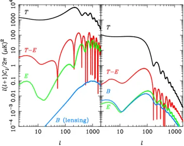
where the labels X andY refer to the temperature (T) and polarisation (E and B) modes that contribute to the total power spectrum. Figure2.1shows that the main contribution to the CMB power spectrum is from theC_lTTtemperature modes from scalar perturbations, so we will focus on these. The transfer functions∆Xl(k)can be written as a line-of-sight integral which contains contributions from the physical sources and geometric projection.

The effects have been well studied mathematically and codes such as CAMB are able to numerically compute theoretical CMB Cls for ΛCDM parameter inputs, as well as a wide variety of other model extensions beyondΛCDM (Lewis et al. 2000;Howlett et al. 2012). The general physical picture is described by acoustic physics. The initial perturbations from inflation cause peaks and troughs in the fluid density field. The matter collapses under gravity but is modulated by the dominant radiation pressure, such that matter oscillates on scales defined by the primordial fluctuations as well as the matter density. This process creates acoustic waves in the fluid with sound speedcs. Between the end of inflation and the end of recombination these imprint a fundamental scale at which matter and photons oscillated and therefore a scale at which they are correlated. Specifically, the longest wavelength oscillation is the first peak inl, with subsequent peaks defined by its harmonics. Generally, the shape of the CMB power spectrum is very sensitive to densities and the primordial power spectrum and recent measurements of the CMB have provided the tightest cosmological constraints available.

2.1.3.3 Matter power spectrum

Measuring the density fluctuations in matter at any point in the universe produces a matter power spectrum. As LSS was seeded by the primordial anisotropies, the matter power spectrum provides another probe of the early universe and its evolution thereafter. As with the CMB, one can write the power spectrum for matter using transfer functions to be computed numerically:

P_m(k)= 4 25 k aH 4 T2 m(k)PR(k), (2.19)

where the transfer functionTm(k) now models the growth of matter fluctuations through the evolution of the universe. It has been shown that at large scales (small k) P ∝ k and that at small scales (largek)P∝k−3. The precise form in between these limits is obtained by solving the full general relativistic Boltzmann equation (Dodelson 2003).

(29)

2.1. The concordance model: ΛCDM ₁₉

FIGURE 4. Temperature (black), E-mode (green), B-mode (blue) and T-E cross-correlation (red) CMB power spectra from scalar perturbations (left) and tensor perturbations (gravitational waves; right). The amplitude of the tensor perturbations is shown at the maximum amplitude allowed by current data (r=0.22 [44]). TheB-mode spectrum induced by weak gravitational lensing is also shown in the left-hand panel (blue; see Sec. 6.1.2).

to constrain gravitational waves since the sampling variance of the dominant scalar

perturbations is large at lowl. Fortunately, CMB polarization provides an alternative

route to detecting the effect of gravitational waves on the CMB which is not limited by cosmic variance [45, 46]; see Sec. 3.

2.7.4. Isocurvature modes

Adiabatic fluctuations are a generic prediction of single-field inflation models. How-ever, multiple scalar fields typically arise in models inspired by high-energy physics, such as the axion model [47], curvaton [48] and multi-field inflation [49, 50]. In such models, if the fields decay asymmetrically and the decay products are unable to reach chemical equilibrium with each other, an isocurvature contribution to the primordial perturbation will result. The simplest, and best-motivated, possibility is an isocurva-ture mode where initially the dominant fractional over-density is in the CDM, with a compensating (very small) fractional fluctuation in the radiation and baryons [51]. The amplitude of the CDM isocurvature mode is quantified by the gauge-invariant quantity

S ≡!c−3!"/4, where!cis the CDM fractional over-density. Generally,S can be

cor-related with the curvature perturbationR, for example in the curvaton and multi-field

models.

In the CDM mode, the photons are initially unperturbed, as is the geometry:!"(0) =

0=#(0)andvb=0. The different equations of state of the CDM and radiation lead to

the generation of a curvature perturbation. On large scales,R grows likeain radiation

Lecture notes on the physics of cosmic microwave background anisotropies March 30, 2009 18

Wednesday, 13 February 2013

Figure 2.1: Breakdown of CMB power spectrum contributions for the T, E and B modes for scalar and tensor perturbations. Typical cosmological values for parameters are assumed. Reproduced fromChallinor & Peiris(2009).

2.1.4 Observing and measuring the universe

Feynman is quoted as saying that “if it doesn’t agree with experiment, it’s wrong.” Fortunately there are numerous high quality datasets available to cosmologists and these have shown very good agreement with the ΛCDM model. To provide a thorough review of all that is available is not within the scope of this short introduction. The aim is to define the datasets that will be used throughout the thesis.

The thesis focusses on datasets which provide likelihood codes as part of the operational output of a mission. Likelihoods are required for mathematical model analysis, to be defined more fully in section3.1. These datasets can easily be split into several categories: measure-ments of the cosmic microwave background radiation (CMB), redshift distance measuremeasure-ments of Supernovae type Ia (SNIa), measurements of the baryon acoustic oscillation (BAO) scale in LSS surveys and BAO measurements in the Lyman-α forest (Ly-α). There are additional measurements that place constraints on the ΛCDM model, these include measurements of the BBN elemental abundances to define the helium fraction and measurements of the local Hubble constant.

Before describing the observations and relevant datasets it is worth noting that measuring distances to objects in astrophysics is a non trivial pursuit which depends on the cosmological model. Both BAO and SNIa data rely on redshift and distance relations to determine universe

(30)

evolution. Pointing a telescope at interesting features on the sky produces light spectra which can be analysed to classify the object studied. Once the absorption line patterns in the spectrum are identified a redshift can be stated which defines the wavelength shift in the signal compared to the known spectral frequency features. Distance is less straight forward to calculate as it requires knowledge about the metric, and therefore a cosmological model is assumed.

As the universe expands with scale factora(t), the distance between two comoving points in spacetime increases. We can define thecomoving distance χfrom the metric of equation (2.2) as the distance between comoving coordinate points in the space-only part of the metric. From the definition of χ, we can defineproper distanceasd=a(t)χwhich measures physical distance between the comoving coordinates at some cosmic time t. However, this proper distance is difficult to measure directly as we are confined to the Earthl. Instead we can define operational distance measurements which relate an observable quantity to distance via a known relation.

With sources of light we know that energy dissipates asr−2and on earth we can measure the flux from a distant source. If we know the energy an object is outputting in a given time frame, its luminosityL, we can calculate the distance via the relationF=L/(4πdL2), wheredL is the luminosity distance. In an expanding universe, however, the area of the sphere itself depends on the scale factor. From the FLRW metric we can see that A=4πS2(χ), whereS2(χ) is defined in equation (2.3), and we can obtain an equation relating flux and luminosity in an FLRW universe. By comparing the FLRW equation for flux to the operational observations of

d_L _{we can relate the luminosity distance to the metric:}

dL(z)=S(χ)(1+z). (2.20)

This relationship describes the luminosity distance we would measure for a given object at z depending on its comoving coordinateχ. We cannot know the comoving coordinate of a source we measure, but instead can calculate it at a given redshift, with the distance depending on the evolution history of the universe:

χ=c

∫ z

0

dz H−1₍_z).

(2.21)

Recalling equation (2.5) and (2.7) we see that the luminosity distance therefore depends heavily on the energy density content of the universe. This is useful, as measurements of luminosity distances can therefore constrain the evolution history of the universe. A similar analysis can be done for the operationally definedangular distancedA: an object of proper diameterlwill subtend an angle on the sky of ∆θ=l/dA, wheredA is the distance to the source. Therefore,

l_{Distance measurements on Earth were originally defined using a metre stick and currently by the speed of}

light. Sadly, in space we cannot lay out rulers to objects and have not enough information about the photon travel time to calculate distance.

(31)

2.1. The concordance model: ΛCDM ₂₁

for an object of known dimension we can measure the angle on the sky between the object’s boundaries and compute the angular distance. Again we can compare to the FLRW metric, where the angular part definesl=a(t)S(χ)∆θand we obtain

dA=

S(χ)

1+z

. (2.22)

Again we see that this relationship depends on the expansion history through χand therefore measurements of dA constrain models of our universe. Note that the luminosity and angular distance are not the same, such that for an object where we know both luminosity and sizea

priori we could compute both distances and be surprised to see that they are not equivalent. In a non expanding universe, however, they would be the same (as redshift would be 0), in line with what is left of our now questionable intuition of these matters. We note too that the comoving distance, and therefore proper distance, would be the same from both measurements and therefore a more intuitive picture of these measurements might be to consider them as reconstructing χ(z).

One can compute a similar distance measure for number density counts of objects, where our knowledge that density is constant in space due to the cosmological principle allows us to relate measured volumes with FLRW metric volume. The various distance measurements discussed allow astronomers to map the universe. Typically different observations are able to measure different scales of distance, and each such measurement will have inherent uncertain-ties. Combining multiple observations allows us to cross-calibrate measurements and create accurate distance measurements across a range of redshifts and using a range of methods, this is known as the cosmological distance ladder. Let us now turn to the datasets which will be used throughout the thesis.

Cosmic microwave background (CMB) radiation measurementsm determine the CMB power spectrum. Experiments for constructing whole sky mappings were conducted by the COBE (Mather et al. 1990)n, WMAP (Bennett et al. 2003;Hinshaw et al. 2003;Spergel et al. 2003) and most recently Planck (Planck Collaboration et al. 2014b,c) satellites. Ground based telescopes focussing on smaller sky regions with a higher resolution include ACT (Fowler et al. 2010;Das et al. 2011) and SPT (Schaffer et al. 2011;Reichardt et al. 2012), whilst some early work was done on balloons. CMB experiments can measure both temperature and polarization of microwave photons across a range of microwave frequencies. The work in the thesis was started in 2013 when WMAP data release 9 (Hinshaw et al. 2013;Bennett et al. 2013) was the state of the art. WMAP was combined with the ACT and SPT datasets which measure smaller scale CMB features (higherl). The Planck satellite 2013 data (Planck Collaboration

m_{The initial discovery of the CMB was by Penzias and Wilson, whilst attempting to remove background noise}

in their detector, and received a Nobel prize.

(32)

et al. 2014b) was released shortly after and still used the WMAP9 polarization data. Planck satellite 2015 data was released nearer the end of the thesis work. Elements of this work have been conducted using each of these 5 datasets and will be stated as appropriate.

We note that the Planck data contains several different datasets (coded into likelihoods) which can be used together or in place of one another (Planck Collaboration et al. 2014a,2016a) (similarly for WMAP). This is due to how the T and E/B mode measurements construct the CMB power spectrum, as discussed briefly in section2.1.3, and also due to the instrumentation used to measureClat low-land hi-l. Additionally there are datasets using gravitational lensing (Planck Collaboration et al. 2016e): photon path distortion by large masses such as dark matter overdensities create distinct signatures that can be used to determine the power spectrum due to lensing. Constraints on the primordial power amplitudeAs, and to a lesser extent the matter density Ωm, can be obtained using only the lensing data.

The WMAP data constrained the CMB angular spectrum between 2 ≤ l ≤ 1200 by measuring temperature and polarisation in 5 frequency bands between 23−93 GHz (effective frequency) between 2001 and 2010. The precision measurements by WMAP reduced the volume of the ΛCDM 6 parameter space by a factor of 68,000 compared to pre-WMAP constraintso. The WMAP data can be combined with the ACT and SPT high multipole ground based experiments. The high-l data extends tol≈10000 but foregrounds are said to dominate abovel≈3000: the useful data range is limited to belowl=3000 (Dunkley et al. 2011).

Planck data extended its satellite-only CMB analysis from 2 ≤ l ≤ 2500 by measuring, with higher resolution instruments than WMAP, the temperature and polarisation in 9 frequency bands covering the 25−1000 GHz spectrum between 2009 and 2013. The Planck 2015 data release is sufficiently precise to not significantly benefit from including other high-l CMB experiments. 2013 Planck data slightly benefits from high-ldata but we have opted to only use Planck in our analysis. It is important to note that the Planck 2013 data analysis introduces 14 parameters which model instrumental noise, foreground signals and other non-CMB sources of power (this is 15 parameters for the 2015 data, whilst the WMAP+ACT+SPT combination uses only 3). These parameters are treated the same as the ΛCDM parameters when constraining parameter values and are termednuisance parameters.

Supernovae Type Ia(SNIa) distance redshift measurements provide measurements ofdL. A type Ia supernovae is generally believed to be a (carbon-oxygen) white dwarf star which accreted matter until it reached a critical mass (the Chandrasekhar mass) and a thermonuclear explosion occurred, at which point it became a supernovae. The exact system producing these is still open to debate (Maoz & Mannucci 2012;Wang & Han 2012) but the property that these systems become supernovae with approximately the same known mass makes them useful for

(33)

2.1. The concordance model: ΛCDM ₂₃

luminosity distance measurements. As the luminosity of these sources is known, they are often referred to as “standard candles”. Their initial usage in cosmology to probe the luminosity distance is credited with identifying the accelerated expansion of the universe (Riess et al. 1998;Perlmutter et al. 1999)pwhich supports the dark energy construction of our models. The measurements typically constrain late time universe evolution and are degenerate in matter and dark energy densities. Combining SNIa data with other probes breaks this degeneracy and provides the tightest constraints on late time evolution. For a short review on constraining models from observations seeAstier(2012).

In this work we use two supernovae catalogues: the Union 2.1 catalogue bySuzuki et al.

(2012) and the joint light-curve (JLA) catalogue by Betoule et al. (2014). The Union 2.1 catalogue consists of 580 supernovae combined from several different supernovae surveys, with a redshift range from z=0 to z≈1.5 (Suzuki et al. 2012, figure 4). The JLA catalogue was available only later on in the thesis. It consists of 740 supernovae combined from multiple surveys with a range of 0.01< z <1.2 (Betoule et al. 2014, figure 8). Some of the supernovae overlap between the two catalogues, such that they cannot be used together, and the JLA catalogue typically provides tighter constraints (Betoule et al. 2014, figure 14).

Baryon acoustic oscillation(BAO) data measures the acoustic oscillations in the power spectrum of matter at a given redshift. The acoustic oscillations are those created by the sound waves at the time of recombination. A very good description can be found inEisenstein et al.(2007) (especially figure 1 describing the power spectrum of various components evolving before and after recombination) and also in the thorough review ofBassett & Hlozek(2009) with informative figures showing various features of BAO on 2D grids. The acoustic oscillations define a preferred scale for matter clustering which can be measured at various redshifts to define an evolution history of the scales of the universe. If the scale is known, then the angular distance can be calculated. BAO are therefore often referred to as “standard rulers”q. BAO measurements have degeneracies between several parameters (such as between Ωm and H0,

between the dark energy equation of state and H0, and within early dark energy models; see Aubourg et al. (2015) for a thorough discussion), and again the best results are obtained by combining datasets.

In this work we use several different BAO measurements. These can be classified into galaxy BAO measurements, where the galaxy matter power spectrum is used, and Lyman-α BAO measurements which measure the intergalactic gas power spectrum using Ly-αemission lines (along the line-sight from high redshift quasar spectra). Aubourg et al.(2015, Table II) summarise the BAO datasets that we have used, with their discussions directly applicable to

p_{Another Nobel prize winning experiment in cosmology, for Perlmutter, Riess and Schmidt.}

(34)

our work. To summarise, we use the galaxy BAO data from the SDSS III BOSS data release 11 (Anderson et al. 2014, DR11) which provides an up to 1% measurement of cosmic distance at redshifts 0.32 and 0.57, with nearly one million galaxies in the redshift range 0.2< z <0.7. We supplement this with the less powerful BAO results ofBeutler et al.(2011, 6dFGS), a 6% distance measurement atz=0.106, andRoss et al.(2015, MGS), a 4% distance measurement at

z=₀._15.

For the Lyman-αdata (Lyα) we use the Lyman-αforest spectra of the BOSS DR11 dataset, specifically we use two independent reductions of this data that can be combined. Note that the specific distance measurements of Lyαare not equivalent to the galaxy BAO distance measured, so the accuracy is not directly comparable, but both distance measures provide similar constraints on cosmological evolution. Firstly we use the auto-correlation BAO measurements of Delubac et al.(2015) (so called forest-forest correlation). These use 140,000 quasars in redshift range 2.1 < z < 3.5 and produce constraints on H0 with 2.6% accuracy (5% on

the distance measured) at a redshift of z=2.34. Secondly we use the quasar-forest cross-correlation BAO measurements ofFont-Ribera et al.(2014), which uses 160,000 quasars over a similar redshift range: a 3% precision onH0, 4% on the distance measure andz=2.36. These

complement the galaxy BAO measurements as they greatly extend the redshift range at which the BAO scale has been measured.

The above three types of dataset define the principal cosmological probes used in this thesis. Each individually has degeneracies within the parameter space, and combining the data