Dipl.-Math. oec Nadine Baumann aus Potsdam
Vom Fachbereich Mathematik der Universit¨at Dortmund
zur Erlangung des akademischen Grades Doktor der Naturwissenschaften
– Dr. rer. nat. – genehmigte Dissertation
Promotionsausschuss
Berichter: Prof. Dr. Martin Skutella Prof. Dr. Ekkehard K¨ohler
Introduction 1
1 Preliminaries 7
1.1 Introduction . . . 7
1.2 Network Flow Models. . . 8
1.2.1 Static Flows . . . 8
1.2.2 Flows over Time with Constant Transit Times . . . 12
1.2.3 Time-Expanded Networks . . . 17
1.2.4 Flows over Time with Flow-Dependent Transit Times . 19 1.3 Submodular Functions . . . 21
1.4 Parametric Search. . . 22
2 A Survey on Evacuation Problems 25 2.1 Introduction . . . 25
2.2 Quickest Transshipment Problems . . . 26
2.2.1 Quickest Transshipments with Constant Transit Times 26 2.2.2 Quickest Transshipments with Inflow-Dependent Tran-sit Times . . . 34
2.3 Earliest Arrival Flow Problems . . . 36
2.3.1 Earliest Arrival s-t-Flows. . . 36
2.3.2 Earliest Arrival Transshipments . . . 38
2.4 Further Methods of Modeling and Optimizing Evacuation. . . 40
3 Earliest Arrival Transshipments 43 3.1 Introduction . . . 43
3.2 Bounded Supplies and Demands . . . 44
3.3 Earliest Arrival Pattern . . . 49
3.4 Constructing the Earliest Arrival Pattern . . . 51
3.4.1 The Structure of the Earliest Arrival Pattern . . . 52
3.4.2 Computing the Earliest Arrival Pattern . . . 56
3.4.3 Reformulation of the Algorithm . . . 60
3.5 Turning the Earliest Arrival Pattern into an Earliest Arrival Transshipment . . . 62
3.6 Tight Earliest Arrival Transshipments. . . 65 i
3.7 Practical Results . . . 68
4 Earliest Arrivals-t-Flows with Flow-Dependent Transit Times 79 4.1 Introduction . . . 79
4.2 Non-Existence of Earliest Arrival s-t-Flows . . . 80
4.3 α-Earliest Arrival s-t-Flows . . . 82
4.3.1 Upper Bound . . . 83
4.3.2 Lower Bound . . . 85
4.4 An Approximation Algorithm . . . 87
4.5 Practical Results . . . 89
5 Data Evacuation on a Path 93 5.1 Introduction . . . 93
5.2 Data Flows . . . 94
5.3 Storage Rules . . . 97
5.4 Determining Optimal Storage Rules . . . 99
5.4.1 Transit Time Excess Paths . . . 99
5.4.2 Capacity Excess Paths . . . 101
5.5 Arbitrary Paths . . . 112
5.6 Practical Results . . . 116
Considering the last few years, the number of evacuations of areas endan-gered by tsunamis or hurricanes, of airplanes having engine turbine prob-lems, of buildings on fire, as well as of evacuations because of bomb alarms has highly increased. The increasing number of emergencies naturally in-creases the interest in an optimal preparation of the evacuation before the emergency occurs. In particular, the heavy interest of the media in the evac-uation test of the newly build airplane Airbus A380 (see for example BBC News Online [7] and Spiegel Online [76]) strengthens the impression that the role of evacuation planning and prediction becomes more important, also in public. While the importance of good evacuation prediction became obvious for the public during the last few years, practitioners and theoreticians were searching for methods to find good evacuation plans for buildings, airplanes, or whole areas for the case of an emergency for a long time.
Besides the large amount of simulation tools for evacuation prediction un-der certain assumptions (see for example [48, 64, 52]), evacuation problems can be modeled as network flow problems. In contrast to static flows, flows over time introduced by the seminal work of Ford and Fulkerson [24, 25] ex-plicitly model the impact of time, which is an important factor in evacuation situations. In this extended model, transit times on arcs indicate the loss of time when traversing a site from one end to the other. Although network flows over time are not capable to map real world behavior exactly to math-ematical models, they offer a good tool to predict the evacuation behavior in existing buildings, airplanes, or areas and to plan new buildings and airplanes with respect to good evacuations.
Given a seat map of an airplane or the locations of working stations in a building together with the building topology, we can model the network. If we can find an optimal evacuation plan in a perfect flow model where pas-sengers are considered to act rational without panic, the evacuation time we determine is a lower bound on the time the evacuee would need. Moreover, it is possible to find a lower bound on the total evacuation time for exam-ple for certain seat maps already in the construction phase of an airplane. Therefore, it is possible to optimize the position of seats and emergency exits in an airplane with respect to evacuation situations.
In typical evacuation situations, the most important task is to get people 1
out of an airplane, an endangered building, or an area as fast as possible. Since it is usually not known how long a building can brave a fire before it collapses, how much time it needs before a smoking aircraft turbine engine really starts burning, or how long a dam can resist a flood before it breaks, it is advisable to organize an evacuation such that as much as possible is saved no matter when the inferno will actually happen. Therefore, it is not enough to only bound the total evacuation time. By sending as much flow as possible into the sinks at each point in time, the uncertainty of the planned evacuation time is taken into consideration. While solutions to thequickest flow problem
minimize the total evacuation time, so called earliest arrival flow problems
aim at optimizing the evacuation process for every point in time. Those and some related flow over time problems such as maximum flows over time are usually referred to asEvacuation Problems (see [35, 36, 38,39]).
Speaking of earliest arrival flows, two main settings are taken into account. On the one hand, the earliest arrival transshipment problem is considered. This network flow problem models especially the airplane evacuation. We know exactly where people are located in a given fixed network topology. Also office buildings with a known amount of working stations fulfill this requirement. The task is to guide them out of the airplane or building as quickly as possible. On the other hand, the earliest arrival s-t-flow problem
is analyzed. Earliest arrival s-t-flows consider the easier model with only one source and one sink but do not give a bound on the number of people to evacuate. In this thesis, we consider these two problems and focus on efficient algorithms for solving them. Further, we do not longer restrict ourselves to evacuation of people but consider the evacuation of data packages in an unstable network.
Earliest Arrival Transshipments. Given a network with multiple sources and multiple sinks with assigned supplies and demands, the quickest trans-shipment problem asks for the minimum time horizon up to which the sup-plies and demands can be satisfied over time. This problem can be solved in strongly polynomial time. The strongly related earliest arrival transshipment problem, which additionally maximizes the amount of flow sent into sinks si-multaneously for each time θ ≥ 0, does not necessarily need to exist in this kind of networks. In order to solve the later problem, we need to restrict to multiple-sources-single-sink networks. Hoppe and Tardos [39] develop an FPTAS for the earliest arrival transshipment problem. Other approaches to solve the earliest arrival transshipment problem strictly restrict the transit times or the capacities of the considered networks. The first exact algorithm to solve the earliest arrival transshipment problem for the
multiple-sources-single-sink setting that runs in time polynomial in the input plus output size is derived in Chapter 3. Using the necessary and sufficient criterion for the feasibility of transshipment over time problems presented by Klinz [50], the earliest arrival pattern can be recursively constructed. In a second step, the earliest arrival pattern is turned into an earliest arrival transshipment by slightly extending the network and applying an algorithm of Hoppe and Tar-dos [40] that computes a quickest transshipment in strongly polynomial time. In particular, the algorithm to compute an earliest arrival transshipment as presented in Chapter 3 is the first algorithm for this problem which does not rely on time-expansion of the network into exponentially many time layers, even in the analysis.
Earliest Arrival s-t-Flows. Given a network with a single source node s, a single sink node t, and a time horizon T ≥0, Ford and Fulkerson [24] (see also [25]) consider the problem of sending as much flow as possible from s
tot by time T; the maximum s-t-flow over time problem. Gale [28], Wilkin-son [77], and Minieka [65] analyzed the problem of maximizing the amount of flow that reached the sink by every time 0 ≤ θ < T; the earliest arrival
s-t-flow problem. The above approaches assume transit times on the arcs to be constant or time-dependent. Whoever has tried to leave a stadium after a soccer game knows that this assumption is far from reality for some real world applications like evacuation or traffic routing. A much more realistic setting is to view transit time as a value that depends on the flow rate, the congestion, or the amount of flow in an arc of the network. In particular, this means that the more flow units are present in an arc the higher is the transit time of this arc. More formally, the transit time of each arc in the network at each time θ depends on the flow on this particular arc at that time θ; so called flow-dependent transit times. Two special models of flow-dependent transit times are considered in this thesis;inflow-dependent transit times and
load-dependent transit times. It has been shown by Gale that earliest arrival
s-t-flows exist for any network with constant transit times. We give examples in Chapter 4, showing that this is no longer true for flow-dependent transit time functions. Here, we restrict ourselves to inflow-dependent and load-dependent transit times. For that reason, we define an optimization version of this problem where the objective is to find flows that are almost earli-est arrival s-t-flows. In particular, we are interested in flows that, for each
θ ∈[0, T), need only α-times longer to send the maximum amount of flow to the sink. Both constant lower and upper bounds on α are given. Further-more, we present a constant factor approximation algorithm for this problem. Finally, we give some computational results to show the practicability of the designed approximation algorithm.
Data Evacuation. Evacuation planning does not only play an important role in human evacuation but also in evacuating data sent through an un-stable network via several processors. Data in the network can be seen as insecure in the sense that it gets lost immediately in case of a disruption. Data that is saved in a processor can be seen as secure, since it can be resent after the disruption. The property that data can be copied is used in order to save copies of data into the processors. The storage capacity of proces-sors is bounded and therefore the storage of data needs to be examined. In Chapter 5, we define the problem and show that we have to concentrate only on the storage rules. Optimal storage rules are determined for special path topologies: transit time excess paths and capacity excess paths. Optimality means that the maximum number of different data packages is stored when considering all nodes of the network. Moreover, it is required that the data packages stored shall be renewed in the sense that there is a steady exchange in the stored data packages in nodes. There also exist an optimal storage rule for arbitrary paths. It can be shown that arbitrary paths are a compound of transit time excess paths and capacity excess paths.
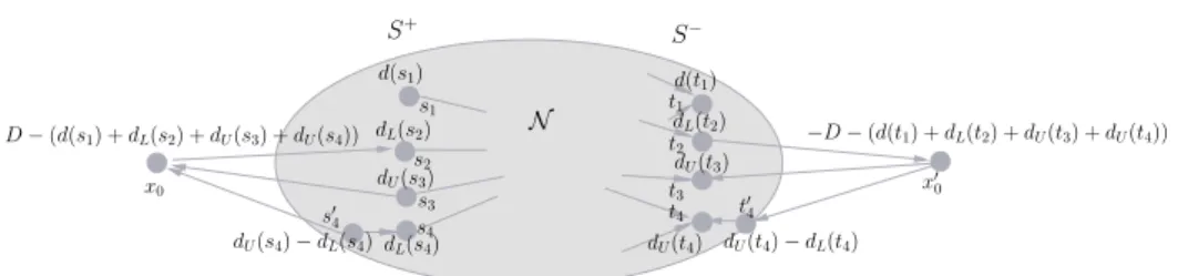
Outline of the Thesis. We define basic notation, introduce network flow models known from literature and give known results in Chapter 1. Moreover, we introduce to two mathematical concepts needed in this thesis; submodular functions and parametric search. In Chapter 2, we formally introduce several evacuation problems considered in this thesis. In particular, we concentrate on known results for the quickest transshipment problem and earliest arrival flow problems. Further, we overview other methods of evacuation predic-tion. An exact algorithm for the earliest arrival transshipment problem is presented in Chapter 3. Before describing the algorithm in detail, we show how to transform networks with supplies and demands given as upper and/or lower bounds into equivalent networks having constant supplies and demands. In Chapter 4, we study the simpler earliest arrival s-t-flow problem for the case that the transit time of each arc in the network at each point in time
θ depends on the flow on this particular arc at the considered time θ. In Chapter 5, we extend the concept of evacuation to non-physical commodities such as data. We consider only networks building a path and show that it is possible to store the maximum number of different data packages along the path, respecting the capacity of storage space. For each possible path topol-ogy, we determine storage rules that define which data needs to get stored in which node.
This thesis tries to be self-contained in the sense that models and al-gorithms used are introduced in detail. Nevertheless, the reader should be familiar with basic graph notation, graph algorithms, optimization problems, and complexity of algorithms. Moreover, a basic knowledge in classical net-work flow theory is advantageous. For a deeper introduction on netnet-work flow models, the reader is referred to the textbooks on combinatorial optimization in general and network flow theory in particular of Ahuja et al. [1], Korte and Vygen [56], and Schrijver [72]. A more detailed introduction in flow over time models is given in the Ph.D thesis of Hoppe [38] and in the survey articles of Aronson [3] and Powell et al. [68]. Several articles of Fleischer, Tardos, and Skutella ([19, 18, 17, 23, 22, 21, 20]) describe special network flow over time problems in detail. A very good introduction to inflow- and load-dependent transit times is given in the Ph.D thesis of Langkau [57] and articles by K¨ohler, Langkau, Hall, and Skutella ([55, 54, 33]). Substantial parts of Chapters 3 and 4of this thesis are already published in [5, 4, 6].
Acknowledgment
Over all, I thank Martin Skutella for evoking interest in new topics of network flow theory, for his help to find new points of view to the considered problems, and for supervising me. I am grateful to the German Science Foundation for the position in the project “Algorithms in Large and Complex Networks” which granted my financial support (grants no. SK 58/4-1 and SK 58/5-3). Following Martin from Berlin to Saarbr¨ucken and later to Dortmund, I had the privilege to work in Prof. Kurt Mehlhorn’s working group at the Max-Planck-Institute for Computer Science and in his own working group at Dortmund University. Furthermore, I was always welcome to the working group of Prof. Rolf M¨ohring at Technical University Berlin and thank him for his hospitality. In particular, it was a pleasure to work together with Ekkehard K¨ohler and Sebastian Stiller.
Especially, I thank Ekkehard K¨ohler for his willingness to take the second assessment to this thesis although he is occupied with many other things.
I would like to thank Sebastian Stiller, Joachim Reichel, and Eric Berberich for their careful and helpful proof-reading and Ingo Schulz for his help pro-ducing some of the practical results. Further, I thank Nicole Megow for being in the same situation and having the same problems.
Finally, I thank all members of the research groups of Prof. Martin Skutella at Dortmund University, of Prof. Kurt Mehlhorn and NWG2 at MPII Saarbr¨ucken, and of Prof. Rolf M¨ohring at TU-Berlin for all the coffee breaks and for being more than just colleges.
Preliminaries
1.1 Introduction
Network flows are an important topic in combinatorial optimization. Not only evacuation settings can be modeled and optimized using network flows but also transportation problems, telecommunication flows, problems of cre-ating timetables, financial flows, and so on.
We define anetworkN = (V, A) to be a directed graph consisting of a set of nodes V and a set of directed arcs A⊆V ×V. We assign a capacity u(a) to each arc determining an upper bound on the amount of flow actually on that arc. Further, we assign arc a a transit time τ(a) representing the time that is needed to traverse the arc. Two concepts of transit times will be considered: constant transit times and transit time functions dependent on flow. Moreover, two specified node sets are considered; sources andsinks. The set of sources is denoted byS+and the set of sinks byS−. The remaining nodes v ∈ V \ (S+ ∪S−) are called intermediate nodes. Sometimes we
are also given a supply-demand function d : S+ ∪ S− → R. It assigns a
positive value, supplyd(s)>0, to each sources ∈S+ and a negative value, demand −d(t)>0, to each sink t∈S−.
Considering evacuation settings, we can observe that each site to evacuate can be represented as such a network. Nodes model rooms in a building, seats in an airplane, crossings of floors, or positions in the aisle of an airplane and so on. Arcs connect locations represented by nodes. They represent the aisle of an airplane, halls, floors, and ways from one room to another in a building. Sources in such a network are sites at which people stay like the seats of an airplane, sleeping rooms of an apartment house, or working stations in an office building. Sinks model safe sites outside the place to evacuate.
In this chapter, we will introduce the notion of network flow models in general. Special network flow models related to evacuation problems are considered in detail. We start by the well studied static flow model in Sec-tion 1.2.1. In Sections 1.2.2 and 1.2.3, we consider several models for flows over time. In this flow model, each arc is given a transit time. Flow is sent through the network continuously and can change its value on an arc over
time. Notice that in earlier work, flows over time were also called dynamic flows. During the last years, the notiondynamic became important in prob-lems where input changes over time or arrives over time. Algorithms solving those problems need to deal with the dynamic input and aim to readjust the solutions to the new information available. The data needed to solve a flow over time problem is available from the beginning. In order to avoid misunderstanding, we always speak of flows over time. This seems to be more intuitive to us and more clear in the parlance of network flows. In Section1.2.4, we describe an even more realistic model of network flows over time. In this model, transit times change with the flow on an arc, i.e., they are flow-dependent. We will discuss two models of flow-dependent transit times;inflow- and load-dependent transit times.
The last two sections of this chapter consider elaborate mathematical concepts which are relevant in this thesis. In Section 1.3, we give a short introduction to submodular functions. In Section 1.4, we briefly introduce the parametric search. This search method finds the optimum value for a given parameter in an optimization problem in strongly polynomial time.
1.2 Network Flow Models
In the following sections, we describe basic properties of the presented flow models. Further, we present results from the literature for two flow problems in the corresponding flow models which form substantial building blocks of the results given in this thesis. In thes-t-flow problem we are given a single-source-single-sink network. The task is to find a feasible flow from source s
to sink t. If we are given a multiple-sources-multiple-sinks network together with a supply-demand functiond:S+∪S− →R, we will focus on the
trans-shipment problem. A transshipment is a flow that fulfills the supplies and
demands of sources and sinks, respectively. The task is to find such a flow, if it exists in the considered network flow model.
1.2.1 Static Flows
Given a network N = (V, A), a function x : A → R+ is called a static flow
function, if the capacity constraintsare satisfied, i.e., it holdsx(a)≤u(a) for alla∈A. A static flow x is said to observe flow conservation in nodev if
X
a∈δ−(v)
x(a) = X
a∈δ+(v) x(a)
holds. Here δ+(v) and δ−(v) denote the set of outgoing arcs of node v and
incoming arcs into node v, respectively. A flow satisfying flow conservation in all nodes is called a circulation. Considering an s-t-flow problem, flow conservation only has to hold for nodes in V \ {s, t}. An s-t-flow fulfilling the required flow conservation equations for nodes inV \ {s, t} and capacity constraints for all arcs is called feasible.
The value of an s-t-flowx is given by value(x) := X a∈δ+(s) x(a)− X a∈δ−(s) x(a) = X a∈δ−(t) x(a)− X a∈δ+(t) x(a) ,
where the second equation follows from flow conservation in all nodes v ∈
V \ {s, t}. An s-t-flow with maximum value is called a maximum s-t-flow. Let X (V be a subset of the nodes. Then we say thatX is ans-t-cut, if s∈X and t ∈V \X. The capacity uof an s-t-cut X is defined as follows:
u(X) := X
a∈δ+(X) u(a) .
Here,δ+(X) denotes the set of directed arcs from nodes in X to nodes inV \
X. If the capacity u(X) is minimal over all sets X ( V, then we call X a
minimum s-t-cut.
The following theorem, called themax-flow min-cut theorem, states a fun-damental relation between the value of a maximums-t-flow and the capacity of a minimum s-t-cut.
Theorem 1.1 (Ford and Fulkerson [24]). For any network, the maximal flow value from s to t is equal to the minimum cut capacity of all cuts separating s and t.
Ford and Fulkerson [24] suggest an algorithm to compute a maximum s
-t-flow. Before describing the algorithm, we give some useful definitions. Given a network N = (V, A) and a feasible flow x, then the residual network Nx = (V, Ax) is defined as follows. Let a = (v, w) be an arc in A.
If x(a) < u(a), then a ∈ Ax. We set the residual capacity of a to ux(a) := u(a)−x(a) > 0. If x(a) > 0, we also insert the backward arc ←−a := (w, v) to Ax having a residual capacity ux(←−a) := x(a). If each arc a is given a
certain costτ(a)∈Rthen the negative of this cost, namely−τ(a) is assigned to the backward arc. A path froms totin the residual network with respect to a flow xis called an augmenting s-t-path.
The algorithm to compute the maximum s-t-flow x starts with the zero flow, i.e.,x(a) = 0 for alla∈A. Then it searches for augmentings-t-paths as long as they exist in the residual networks with respect to the actual flow x. Along such an s-t-path, flow amounting to the minimal residual capacity γ
is augmented, i.e., we increase x(a) by γ, if a is a forward arc on the path, and we decrease x(a) by γ, if its backward arc ←−a is part of the path. Since
γ is chosen as the minimal residual capacity along this path, we guarantee capacity constraints and non-negativity constraints x(a) ≥ 0 for all a ∈ A. Unfortunately, the total number of paths found can be exponentially large.
An s-t-flow x :A → R+ defines a flow on arcs. Since the overall goal is
to optimize an evacuation problem, we need to determine paths along which people can leave a site to evacuate. Therefore it is advantageous, if we can give a formulation of the flow on a set of paths P from s to t. It is well known that the flow function x defined on arcs can be decomposed into a flow on at most |A| paths P and cycles C in N together with non-negative flow values x(P) for P ∈ P ∪ C. For those values on paths and cycles, the following property has to hold:
x(a) = X
P∈P∪C: a∈P
x(P) for all a∈A.
We call the set P together with the flow values x(P) for P ∈ P a path de-composition, ifC =∅. Algorithmically, the path decomposition can be found by using the algorithm for finding a maximum s-t-flow backwards. There-fore, we only consider the network consisting of arcsa∈A having a positive value x(a). In this restricted network N0, we set the capacity u0(a) := x(a)
and apply the algorithm to find a maximum s-t-flow in N0. Thereby, at
least one arc is expunged from the relevant networkN0 in each iteration and
therefore maximal|A| many paths can be found. The resulting set of paths together with the corresponding minimal residual capacity builds the path decomposition. Flow that is still on cycles can be ignored since it does not increase the amount of flow sent from node s to t.
Another important static flow problem, which will be needed throughout this thesis, is the min-cost circulation problem. Assume we are additionally given a cost function τ : A → R on the arcs. The cost of a circulation x is defined as:
cost(x) :=X
a∈A
The min-cost circulation problem looks for a feasible circulation x having minimum cost cost(x). In the following, we describe how to solve the min-cost circulation problem to optimality in network N. Therefore, we use the optimality criterion of Klein which suggests an algorithm.
Theorem 1.2 (Klein [49]). A flow x is a min-cost circulation if and only if there is no directed cycle C in the residual network Nx such that the
sum of the cost around C’s arcs is negative. A directed cycle is a sequence of distinct directed arcs of the form {(v0, v1),(v1, v2), . . . ,(vk, v0)} involving distinct nodes.
The naturally induced algorithm, of course, does the following. To com-pute the min-cost circulation, we start in network N with the zero flow. By successively searching for cycles having negative cost as long as they exist in the corresponding residual networks, we increase the flow on those cycles. Once we find such a cycle, we augment flow of value of the minimal residual capacity γ along the cycle.
If flow on cycles of zero length is added to the circulation, the cost does not increase but the amount of flow in the network increases. We will call a min-cost circulation that maximizes the amount of flow in the network
min-cost (maximum) circulation.
Zadeh [78] gives bad examples for this algorithm for which the algorithm indicated by Klein has an exponential running time in worst case. The al-gorithm requires 2n+ 2n−2 −2 augmentations in a network having 2n+ 2
nodes for n ∈ N. The minimum mean cycle-canceling algorithm presented by Goldberg and Tarjan [29] has a strongly polynomial running time. A sur-vey on the complexity of min-cost circulation algorithms can be found in the book of Schrijver [72].
A related problem is the problem of finding a min-cost s-t-flow. There the goal is to compute a min-cost circulation in the network extended by an arc (t, s) with specified cost τ(t, s). There can be several circulations having minimum cost in such a network. Depending on the problem, we are sometimes seeking the one with highest flow value on arc (t, s); themin-cost
(maximum) s-t-flow. Here, flow on zero length cycles needs to be added.
Notice that the cost of such a circulation stays the same while the amount of flow in the network increases.
We define thecost of the min-cost s-t-flowxdependent on the cost of the additional arc (t, s):
costτ(t,s)(x) := X a∈A∪{(t,s)} τ(a)x(a) =X a∈A τ(a)x(a) +τ(t, s)x(t, s) . (1.1)
Another problem related to evacuation is thetransshipment problemwhere we are given multiple sources and multiple sinks in the network. The supply-demand-function d : S+∪S− → R assigns a positive supply to each source
in S+ and a negative demand to sinks in S−. Considering a transshipment problem, flow conservation has to hold only for nodes w ∈ V \S+ ∪S−.
For nodes v ∈ S+∪S− the flow function x has to satisfy the supplies and
demands, that is X a∈δ+(v) x(a)− X a∈δ−(v) x(a) =d(v) .
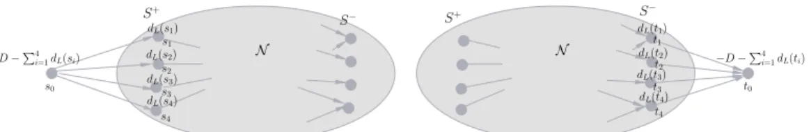
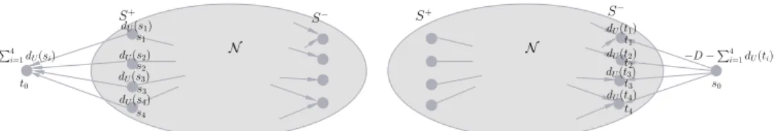
Such a transshipment problem in a network with multiple sources and mul-tiple sinks can be reduced to an s-t-flow problem by a slight network trans-formation. We add asupersource swith arcs (s, s0) for alls0 ∈S+ and assign a capacity of d(s0) to this arc. For each sink t0 ∈ S− we insert arcs (t0, t) to a new sink node t which will be called the supersink. We assign a capacity of −d(t0) to those arcs. A feasible s-t-flow with value P
s0∈S+d(s0) in the modified network naturally induces a feasible flow in the original network satisfying all supplies and demands. Each maximum s-t-flow obviously has the demanded flow value. Thus, when considering static flow models, we can restrict ourselves to networks with a single source and a single sink.
1.2.2 Flows over Time with Constant Transit Times
In various well known static flow problems one seeks a functionx:A→R+
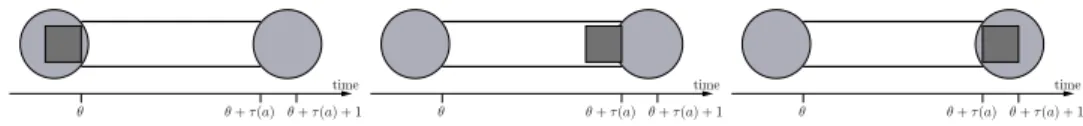
that assigns a flow value x(a) to an arc a. In contrast to that, a flow over timef is a function on A×R where the second parameter denotes the time component – f(a, θ) describes the flow on arc a at time θ. This flow can be interpreted as flow rate, i.e., the amount of flow entering the particular arc per time unit. The flow rate entering an arc is bounded by the capacity of that arc, i.e., f(a, θ) ≤ u(a). Considering flows over time, we need to introduce a time component into the network itself. Therefore, we assign a constant transit time τ(a) to each arc a= (v, w). This value determines the time that flow needs to traverse the arc from the start node v to the target nodew. Moreover, sending one unit of flow into the arc at flow rate one at time θ means, that at time θ +τ(a) flow of rate 1 enters the target node
θ+τ(a) θ time θ+τ(a) + 1 θ θ+τ(a) θ+τ(a) + 1 time θ+τ(a) + 1 θ time θ+τ(a)
Figure 1.1: Arc having a capacity of one unit of flow per time unit. Each unit of flow entering that arc at timeθstarts leaving the arc at time θ+τ(a). It totally has left the arc at timeθ+τ(a) + 1.
of the arc. The whole flow unit has left the arc another time unit later at time θ+τ(a) + 1 (see Figure1.1 for clarification).
The flow function f has to satisfy flow conservation constraints not only in every node w∈V \(S+∪S−), but also at every time θ∈R. Notice that the flow ratef(a, θ) determines the amount of flow entering arc a at time θ. The flow rate entering node w at time θ from an arc a ∈ δ−(w) is thus determined by the flow rate entering that arc at time θ −τ(a). Therefore, the flow conservation constraint in node w is defined as follows:
X a∈δ+(w) Z θ −∞ f(a, θ)dθ ≤ X a∈δ−(w) Z θ −∞ f(a, θ−τ(a))dθ .
Equality is not required in order to allow flow to be stored in nodes of the network. Note that some algorithms for flows over time explicitly forbid storage of flow in nodes whereas others only have a bounded capacity of node storage. We allow storage of flow at nodes in principle and without upper bounds on the amount. However, the algorithms used in this thesis do not make use of the storage opportunity; they send the flow through the network without storing flow at any of the non-source nodes.
A flow over time f, satisfying the flow conservation constraints in all required nodes, is said to be feasible, if for all arcs a and every time θ:
f(a, θ) ≤ u(a) holds. For a given time horizon T, we further require that there is only flow in the network during the time interval [0, T). Since flow entering arca= (v, w) at timeθreaches nodewat timeθ+τ(a), we especially require f(a, θ) = 0 for all θ /∈ [0, T −τ(a)). This guarantees that there is no flow in the network before time zero and that at time T all flow has left the network. The flow conservation constraint of each node w needs to be satisfied only within this time interval:
X a∈δ+(w) Z T 0 f(a, θ)dθ ≤ X a∈δ−(w) Z T 0 f(a, θ−τ(a))dθ .
Notice that it would not be necessary to subtract the transit time of the con-sidered arc in the set of all incoming arcs. By the assumption thatf(a, θ) = 0
forθ /∈[0, T −τ(a)) the compared values stay the same if we require: X a∈δ+(w) Z T 0 f(a, θ)dθ ≤ X a∈δ−(w) Z T 0 f(a, θ)dθ .
An s-t-flow over time naturally requires the flow conservation only in nodes in V \ {s, t}. Thevalue of ans-t-flow over timef with time horizon T
is defined by the net flow value that leaves the source over all time steps or enters the sink over all time steps θ∈[0, T).
value(f) = X a∈δ+(s) Z T 0 f(a, θ)dθ− X a∈δ−(s) Z T 0 f(a, θ)dθ = X a∈δ−(t) Z T 0 f(a, θ)dθ− X a∈δ+(t) Z T 0 f(a, θ)dθ
If the value is maximized, we speak of a maximum s-t-flow over time. In the following, we will denote the value of a maximum flow out of source s
reaching sinktfor a time horizonT also byoT({s}), if we are not considering
a concrete flow f.
More formally, the functionoθ(X) determines the maximum value of flow over time that can be sent out of sources inX to sinks not in X by time θ ∈
R+. Sinces is the single source andt the single sink:
oT({s}) = max{value(f)|f feasible s-t-flow with time horizon T}.
This function is used throughout this thesis for the different settings.
Various results for this flow over time model with constant transit times are known. One of the most remarkable ones is a theorem by Ford and Fulkerson [24] together with an argument for continuity by Anderson and Philpott [2] on maximum s-t-flows over time for the time horizon T.1 Ford
and Fulkerson introduce a special class of flows over time, which resembles static flows. They define atemporally repeated flow to be a static flowxthat is decomposed into flows on paths in network N. Let P be the set of paths and x(P) the non-negative flow values on paths P ∈ P such that the length of each path is bounded from above byT. A temporally repeated flow repeat-edly sends flow over the paths ofP as long as this flow can reach the sink be-fore timeT, i.e., it starts sending flow at time zero and stops at timeT−τ(P). Obviously, such a flow is a feasible flow over time. It naturally obeys flow
1Note that Ford and Fulkerson considered a discrete flow model where time is being
conservation and capacity bounds by the nature of the path decomposition and the feasibility of the static flowx, namelyP
P∈P:a∈Px(P) =x(a)≤u(a).
By definition, no flow is in the network before time zero and after time T. The following lemma determines the value of the temporally repeated flow froms to t in terms of the static flow x.
Lemma 1.3. The value of a flow over timef that is computed as a tempo-rally repeated flow of a static flowx equals:
value(f) = X
P∈P
(T −τ(P))x(P) = T ·value(x)−X
a∈A
τ(a)x(a) . (1.2)
Observe that the flow value is independent of the path decomposition P. One natural goal is now to find a temporally repeated flow having maximum flow value. The existence of such a kind of maximum s-t-flow over time is given by Ford and Fulkerson [24] (see also [2]).
Theorem 1.4 (Ford and Fulkerson [24]). There always exists a tempo-rally repeated flow that is a maximum s-t-flow over time. Such a temporally repeated flow can be computed using a static min-costs-t-flow.
Notice that the value of the maximum s-t-flow over time for time hori-zon T, i.e., oT({s}), determined as in in (1.2), equals −costT(x), i.e., the
negative of the cost of a static min-cost circulation in network N extended by an uncapacitated arc (t, s) with cost −T (compare equation1.1). Here,x
denotes the static min-costs-t-flow computed in networkN where the transit times are interpreted as costs. The choice of−T as cost of the additional arc bounds the length of the used paths by T and therefore the time horizon is obeyed. Further, we know that the static flow x and the flow value value(x) are integral if all capacities are integral.
Analogously to the static case, we define a transshipment over timeto be a flow in a multiple-source-multiple-sink network where given supplies and demands now have to be satisfied over time. Flow conservation only has to hold for nodes w∈V \(S+∪S−). For nodes v ∈S+∪S− the outgoing and incoming flow over time has to equal the supply and demand, respectively, i.e., X a∈δ+(v) Z T 0 f(a, θ)dθ− X a∈δ−(v) Z T 0 f(a, θ)dθ =d(v).
Discrete Flows over Time. The above described flow model is also called
continuous flow over time model. When Ford and Fulkerson introduced the
θ+τ(a) time θ
Figure 1.2: Arc with transit timeτ(a) in a discrete flow over time model. Flow units leaving a node via arc a at time θ ∈ {0,1, . . . , T −1−τ(a)} totally have left arc a at timeθ+τ(a).
sending flow at (continuous) flow rates, they send packets of flow units at discrete points of time into the arcs. In this model, not the continuous time interval [0, T), but all discrete time steps {0,1, . . . , T −1} are considered. That means we are looking for a flow function f : A× {0,1, . . . , T −1} →
R+. The flow rate f(a, θ) on arc a = (v, w) determines the amount of flow
that is sent into arc a at time step θ ∈ {0,1, . . . , T −1}. Flow units sent into an arc a at a time θ totally reach the target node w of that arc at time θ+τ(a). Here, τ(a) denotes the transit time of arc a (see Figure 1.2 for a better understanding of the difference to continuous flows). In such a model, obviously, all transit times need to be integral. Consequently, it suffices to consider integral time horizons.
Flow conservation can be adapted directly to the discrete case. Instead of integrating, it suffices to sum over the considered time steps{0,1, . . . , T−1}. Thus, flow conservation in nodev is obeyed in the discrete model, if
X a∈δ+(v) T X θ=0 f(a, θ)≤ X a∈δ−(v) T X θ=0 f(a, θ) holds.
In the discrete model, the flow value of an s-t-flow over time can be described by summing up the flow leaving the source s in each time step or entering the sinkt in each time step, i.e.,
value(f) = X a∈δ−(t) T X θ=0 f(a, θ)− X a∈δ+(t) T X θ=0 f(a, θ) = X a∈δ+(s) T X θ=0 f(a, θ)− X a∈δ−(s) T X θ=0 f(a, θ) .
S+∪S−, i.e., X a∈δ+(v) T X θ=0 f(a, θ)− X a∈δ−(v) T X θ=0 f(a, θ) =d(v) must hold.
As indicated before, many results made for discrete flows over time can be generalized to continuous flows over time. A similar interrelation can be made about the two flows itself. Assume we are given a feasible discrete flow over time f for time horizon T with flow f(a, θ) entering arc a ∈ A
at time θ ∈ {0, . . . , T − 1− τ(a)}. This discrete flow over time can be interpreted as a continuous flow over time f0 by sending flow of rate f(a, θ) into arc a during the whole time interval [θ, θ+ 1), i.e., f0(a, θ0) := f(a, θ) forθ0 ∈[θ, θ+1) and for alla∈A. The capacity constraints of the continuous flow over time are obviously obeyed, since f(a, θ)≤ u(a) induces f0(a, θ0)≤
u(a) for all θ0 ∈ [θ, θ+ 1). This interrelation is a bidirectional one, if the time horizon and all transit times of network N are integral. Suppose we are given a feasible continuous flow over time f0 computed in network N
with time horizon T. Then this flow f0 can also be interpreted as a discrete flow over time f. We set the flow on arc a at discrete time θ to the total flow that has entered arc a during the time interval [θ, θ + 1) in f0, i.e.,
f(a, θ) :=Rθθ+1f0(a, θ0)dθ0 for allθ ∈ {0, . . . , T−1−τ(a)}for alla∈A. The capacity constraints are obeyed since
f(a, θ) = Z θ+1 θ f0(a, θ0)dθ0 ≤ Z θ+1 θ u(a)dθ0 ≤u(a)
holds. The first inequality follows from the feasibility of the continuous flow over timef0.
1.2.3 Time-Expanded Networks
Flows over time are more complex than static flows in the sense that the flow is specified for all times θ ∈ [0, T). Klinz and Woeginger [51] observed, for example, that there does not exist a deterministic polynomial time algorithm that solves the min-costs-t-flow over time problem with given supply. In this problem, we search for a flow that sends the total supply over time into the sink within a given time horizonT. The corresponding static flow problem is easy to solve as described in Section1.2.1. If all transit times are integral2, we 2In case of rational transit times scaling helps to fulfill the integrality assumption.
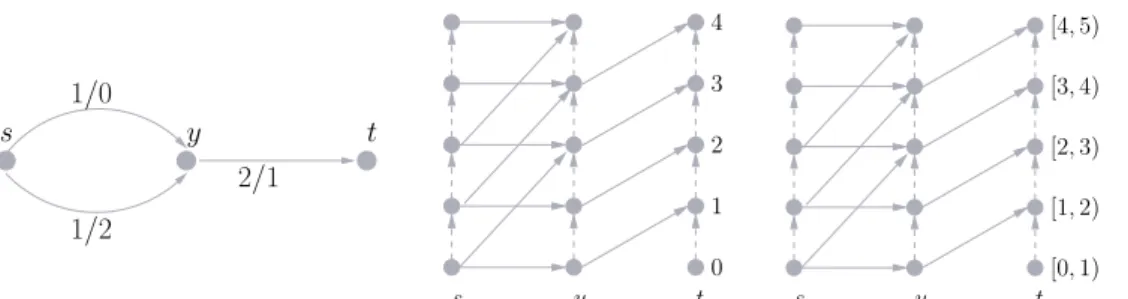
t y s 2/1 1/2 1/0 2 1 3 4 s y 0 t [2,3) [1,2) [3,4) [4,5) s y [0,1) t
Figure 1.3: Network and its time-expanded version (discrete and continuous) for a time horizonT = 5, including holdover arcs. The arc notation denotes capacity/transit time.
can directly apply the algorithm for the static flow problem in an extended network. This special network acts as a static representation of the flow over time model where only integral points in time are considered. Ford and Fulkerson [24] introduced the so called time-expanded network in which the flow over time problem can be solved in pseudo-polynomial running time using static flow algorithms.
A time-expanded network with time horizon T consists of T copies of the node setV, one for each time unit. We call such a copy atime layer. For each arc a = (v, w) of the network N having transit time τ(a), an arc is inserted between the copy of nodev in time layerθ ∈ {0, . . . , T −1−τ(a)} and the copy of node w in time layer θ +τ(a) into the time-expanded network NT
(see Figure 1.3). We denote the copy of node v in time layer θ as v(θ) and the copy of nodewin time layer θ+τ(a) as w(θ+τ(a)). If we allow storage of flow in nodes, holdover arcs are needed that connect the copy of node v
in time layer θ to the copy of node v in the next time layer. The set of holdover arcs consists of all arcs (v(θ), v(θ+ 1), for all θ ∈ {0, . . . , T −2}. One other application for the use of holdover arcs is the existence of sup-plies and demands at sources and sinks in the original network. In order to satisfy all supplies and demands over time, sometimes flow units have to wait before leaving the source. In such a case, holdover arcs are inserted into the time-expanded network for all sources and all sinks. The supply d(s0) for each source s0 ∈ S+ is assigned to node s0(0) in the time-expanded
net-work. The demand d(t0) for each sink t0 ∈ S− is assigned to node t0(T −1) in the time-expanded network. Network NT is obviously a static network
as defined in Section 1.2.1 and the use of known algorithms for static flow problems is possible. In this network we can solve the static transshipment problem again by inserting a supersource and a supersink. The insertion of supersource and supersink works analogously to the case of static network flow models.
A flow in a time-expanded network can directly be transformed into a dis-crete flow over time and vice versa. Assume we are given a static flow x(a) on arcs in NT. Each arc a in NT corresponds to an arc a0 in network N.
Let the start node of arc a be in time layer θ. We define a flow over time on arc a0 at time θ to have flow rate f(a0, θ) := x(a). This flow is feasible by construction. The interpretation of a discrete flow over time as a static flow in the time-expanded network works exactly the other way round. By the interrelation between discrete and continuous flows over time as described in the previous section, we can also interpret the flow computed in the time-expanded network as a continuous flow over time. Then, each time layer represents a time interval instead of a point in time. Static flow on an arc with target node in time layer θ is now interpreted as flow arriving at this node during the time interval [θ, θ+ 1). Analogously, static flow on an arc with start node in time layer θ is now interpreted as sent out of this node during the time interval [θ, θ+ 1). See on the right hand side in Figure 1.3 for the interpretation in the time-expanded network.
A drawback of the time-expanded network is that the size of the network depends on T. Even polynomial time algorithms for static flow problems become pseudo-polynomial, if they are applied in the time-expanded network. This is indicated by the following theorem.
Lemma 1.5. Given a network N with n nodes and m arcs. The time-expanded network NT consists of T n nodes and (n+m)T −n−P
a∈Aτ(a)
arcs where T is the considered time horizon.
Nevertheless, time-expanded networks are not only useful for problems for which no flow over time algorithm is known but they are also useful proving the correctness of a given algorithm. Ford and Fulkerson, for example, proved the correctness of their maximums-t-flow over time algorithm by determining a cut in the corresponding time-expanded network.
1.2.4 Flows over Time with Flow-Dependent Transit Times
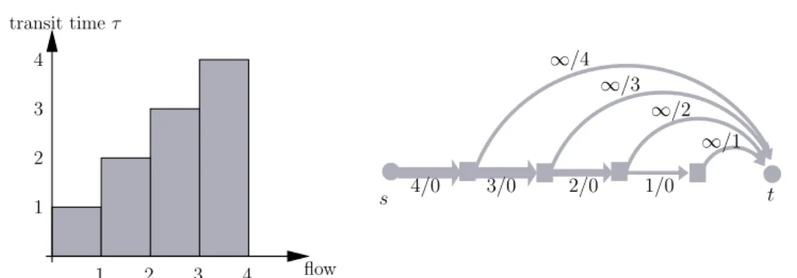
While flows over time are much more appropriate to model real-world situa-tions than static flows, often the constant transit times do not model reality in a sufficiently precise way. For example, it can be easily observed that there is a high correlation between the congestion of a hallway, staircases, or an aisle in an airplane and the time needed to traverse it. A more accurate method for describing this correlation is provided by the use offlow-dependent transit times instead of constant transit times. For this purpose, we will assume in
the following that a transit time functionτ :A×R+→R+ is given as a
left-continuous and non-decreasing function of the flow on arcs. Here, in contrast to the model with constant transit times, we are given a second parameter that refers to the flow.
Flows over time with flow-dependent transit times have been studied be-fore. Merchant and Nemhauser [63] suggest a model where for every arc there is both a flow-dependent cost function and a so called exit function that determines the amount of traffic that can leave the arc in dependence of the amount of flow on that particular arc. Although, their model was both nonlinear and non-convex and thus difficult to handle for efficient algorithms, it was influential for many other results in this area. Carey and Subrahma-nian [11] introduce a model that uses an approach similar to time-expanded networks for the case of flow-dependent transit times. In this model, not only the arcs are expanded over time but also by several states of the transit time function.
In literature on flow dependent transit times, different options of modeling them are described. We will briefly describe two known models, that we will make use of in the sequel.
On the one hand, we considerinflow-dependent transit timesas described in K¨ohler, Langkau, Skutella [54]. In this model, the transit time is a function of the rate at which the flow is entering the arc a at time θ. In particular, flow entering arcaat the flow ratef(a, θ) needs a transit time ofτ(a, f(a, θ)) to traverse the arc. Hence, flow units entering an arc at the same time have the same speed (defined by the transit time of the arc) and, while traversing the arc, their speed stays constant. This transit time model allows a comparably easy description of the dependency between flow and transit times. However, it has the disadvantage that there can be situations where flow entering at a small flow rate can pass flow units that entered the same arc at a higher flow rate before—the so called first-in-first-out (FIFO) property is not fulfilled. What makes this model somewhat difficult to handle is, that we have to guarantee that the network is empty after timeT. More precisely, whenf(a, θ)>0, it must hold that θ+τ(a, f(a, θ))< T. The conditions on flow conservation constraints and supply/demand requirements have to be adapted to take this property into account.
On the other hand, a more precise account of transit times that depend on the flow in some real applications is to assume that the transit times depend not only on the amount of flow entering an arc but also on the amount of flow currently being in the whole arc. K¨ohler and Skutella [55] describe this kind of transit time function called load dependent transit times. In this model, the total amount of flow on an arc a at a time θ is used as the input to the transit time functionτ; this amount of flow is called the load of the arc.
Since the flow on an arc changes continuously, also the transit time of the arc changes with each unit of flow entering or leaving the arc. Note that at each moment all units of flow on an arc have the same speed.
Although both of the above models cannot describe evacuation flows in their whole complexity, they are however capable of modeling at least some important aspects of evacuees behavior.
1.3 Submodular Functions
In Chapter3of this work, we consider submodular functions. Since submod-ular functions are of general interest, we give a definition and some properties of submodular functions. After that, we briefly survey existing algorithms for submodular function minimization.
Definition 1.6. LetE be a finite set. Any function ρ: 2E →Z satisfying
∀X, Y ⊆ E :ρ(X) +ρ(Y)≥ρ(X∪Y) +ρ(X∩Y) (1.3) is called submodular function. A function for which strict equality holds is called modularfunction.
A well known example of submodular functions is the capacity func-tion u : 2V → R+ of an s-t-cut. This can easily be proven by checking
equation (1.3). The following lemma gives some easy to check properties of submodular functions which we will need.
Lemma 1.7. Let ρ, φ : 2E → Z be submodular functions and ψ : 2E →Z a modular function. Then the following holds:
1. The function a: 2E →Z defined asa(X) := ρ(X) +φ(X) for X⊆ E is submodular.
2. The function b : 2E →Z defined asb(X) := ρ(X)−ψ(X) for X ⊆ E is submodular.
Minimizing Submodular Functions. The first combinatorial but pseudo-polynomial time algorithm was already given in 1985 by Cunningham [16]. Here the submodular function can be minimized in time polynomial in |E|
and max|ρ(X)|.
The first polynomial time algorithm to minimize submodular functions without any side constraint was given by Gr¨otschel, Lovasz, and Schrijver [30] in 1988. They use the Ellipsoid Method by Khachiyan [47] which solves linear programs in strongly polynomial time. This algorithm is not combinatorial
and for a long time there has not been found a combinatorial, strongly poly-nomial time algorithms to minimize submodular functions.
Nearly at the same time, Iwata, Fleischer, and Fujishige [43] and Schri-jver [71] found combinatorial, strongly polynomial time algorithms. Both al-gorithms are based on the fundamental work by Cunningham [15,16]. Iwata improved in [42] the algorithm of Iwata, Fleischer, and Fujishige to be even fully combinatorial.
A wide survey of the different minimization algorithms and several im-provements is given by McCormick [59]. More details and background infor-mation on submodular functions in general are given in Fujishige [26].
1.4 Parametric Search
In his seminal paper, Megiddo [62] describes an algorithm for a search method called parametric search. We are given a parameterized instance of a certain problem, i. e., an optimization problem or a feasibility problem. Such a parameterized instance is allowed to contain one linear parameter. A solution to a parameterized algorithm now consists of an assignment of values to the variables of the instance and, additionally, a value for the given parameter such that the problem is optimal or feasible, respectively. Megiddo shows that the value for the parameter can be found in strongly polynomial time, if there exists an “easy” algorithm for the non-parameterized problem that runs in strongly polynomial time. In the following, we show how this parametric search works and enumerate the requirements for such an algorithm to be called “easy”.
We are given a parameterized instance of a certain problem where a linear parameterλis part of the instance. The parameter has to be known to lie in an interval I ⊆ (−∞,∞). Further, we assume that we are given a strongly polynomial algorithm A for the considered problem. We require that the steps of A are only of one of the following three types: additions, scalar multiplications, and comparisons.
Using the parameterized instance, the algorithm A has to be adapted to be a parameterized version. In the adapted version not only values ai
and aj have to be added, multiplied by a scalar c, or compared, but linear
functionsai+λbi and aj +λbj.
Addition of linear functions ai +λbi +aj +λbj reduces to additions of
known values (ai+aj)+λ(bi+bj), as well as scalar multiplicationc(ai+λbi) =
(cai) +λ(cbi) reduces to scalar multiplication of known values and conserves
the linearity. Therefore, the knowledge of the value of λ is not necessary. The comparison of linear parameterized functions is more difficult without
knowing λ. By simple computation of the intersection point of two linear functions ai +λbi and aj +λbj, the critical value λ∗ for which ai +λ∗bi =
aj +λ∗bj can be found. If there is no critical value or the value of λ∗ does
not lie in the feasible interval I, the result of the comparison is independent of λ. The result of the comparison thus can be determined immediately. If the value λ∗ lies in I, we have to check whether it is too high or too low for a feasible value of λ. This check can be done using the strongly polynomial algorithmA on the non-parameterized problem where the parameter is fixed toλ∗. Then the outcome is analyzed, for example by comparing the objective values for the actual choice of λ∗ and the one from the last iteration or checking the existence of a feasible solution, respectively. If λ∗ was too low, we substitute the lower bound of interval I by λ∗, if it was too high, we substitute the upper bound.
Megiddo [62] shows that the number of tests for λ∗ can be bounded by the number of comparisons done by the algorithmAfor a non-parameterized problem. Since A is used as a subroutine whenever a comparison is done, the total running time of A for a parameterized problem lies in the running time of algorithm A for the non-parameterized problem times the number of the comparisons of A. Thus, if the running time of algorithm A for the non-parameterized problem is strongly polynomial, the running time of the algorithm for the parameterized version will be strongly polynomial, too.
Throughout this thesis, all algorithms used together with parametric search fulfill the requirements that only additions, scalar multiplications, and comparisons are necessary. Further, only linear parameters are used.
A Survey on Evacuation Problems
2.1 Introduction
The task of evacuation problems is to send the maximum number of people to evacuate from a dangerous site to safe sites. Obviously, the parameter time plays an important role in evacuation problems. Therefore, only flow over time models are considered to model the evacuation setting in a reasonably realistic way. Quickest transshipment problems are analyzed in order to get a reasonable lower bound for the minimum time horizon of a real evacuation situation and is therefore of high relevance. Given an amount of supplied and demanded flow in source and sink nodes the quickest transshipment problem asks for a flow that sends this amount of flow over time from sources to the sinks in the minimum possible time horizon. In the context of emergency evacuation from buildings, Berlin [8] and Chalmet et al. [12] study the quick-est transshipment problem in networks with multiple sources and a single sink. Jarvis and Ratliff [44]1 showed that three different objectives of this
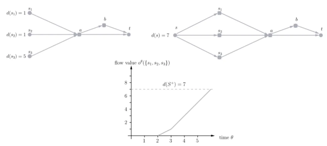
optimization problem can be achieved simultaneously: (1) Minimizing the to-tal time needed to send the supplies of all sources to the sink, (2) maximizing the amount of flow leaving the network at all timesθ ≥0, and (3) minimizing the average time for all flow needed to reach the sink. Each transshipment optimizing objective (1) is a quickest transshipment. Objective (2) says that it is additionally possible to simultaneously maximize the amount of flow sent into the sink up to all times θ≥0 in a transshipment problem. A transship-ment optimizing objective (2) is called earliest arrival transshipment. Each earliest arrival transshipment obviously additionally optimizes objective (1) and is therefore a quickest transshipment. The reverse does not hold, i.e., not every quickest transshipment optimizes (2), too. Notice that earliest arrival transshipments do not necessarily exist in networks with multiple sinks, but quickest transshipments do. Besides, each transshipment maximizing objec-tive (2) naturally minimizes objecobjec-tive (3). We will not consider objecobjec-tive (3) in the following, since we concentrate on objective (2), maximizing the
1Strictly speaking, Jarvis and Ratliff [44] only consider the single-source case but their
observation also applies to the more general case with multiple sources.
amount of flow leaving the network at all times θ ≥0, in this thesis.
Not only transshipment problems but also maximum s-t-flows over time problems can be considered in order to model different evacuation settings. The task is to send as many people out of an endangered site. Again, it is preferable, if the computed maximum s-t-flow has the property, that it also maximizes the amount of flow sent into the sink up to each timeθ ≥0. Therefore, earliest arrival s-t-flows are considered. An evacuation fulfilling the earliest arrival property is known to be optimal, even if the catastrophe occurs before all people have left the site to evacuate, since the number of evacuated people by then is as large as possible.
In the following, we will give a survey on the above mentioned network flow problems and state known results as well as algorithms. In Section 2.4 we overview further methods of solving evacuation problems.
2.2 Quickest Transshipment Problems
In the following, we considerquickest transshipment problemswhich are stud-ied very well, i.e., problems where objective (1) is optimized. An instance of the quickest transshipment problem consists of a networkN with capacities and transit times on the arcs, multiple source nodes S+ and multiple sink
nodes S− with a supply-demand function d : S+∪S− → R. The task is to
determine the minimum time horizonθ∗ for which there exists a feasible flow satisfying all supplies and demands as well as to find such a feasible flow. In the following, we will give a short overview over results for the quickest transshipment problem for several network flow models.
2.2.1 Quickest Transshipments with Constant Transit Times
For an instance of the quickest transshipment problem with constant transit times, we further require that capacities and transit times on arcs are constant and integral. If capacities and transit times are not integral, scaling helps to fulfill this property.
There exists an easy to see algorithm in the time-expanded network to determine a quickest transshipment. For such an algorithm, we first guess an (integral) time horizonθand construct the time-expansion of networkN. We add a supersources which is connected to each copys0(0) of sources s0 ∈S+
at time layer zero by a zero transit time arc having capacity d(s0). Further, we add a supersink t to the network with uncapacitated, zero transit time arcs (t0(θ−1), t) for all copies oft0 ∈S−at time layerθ−1. Using a maximum static s-t-flow computation in this network, we compare the resulting flow
value with the total supply of the problem. If the flow value is smaller than the total supply, we need to increase the guessed time horizon. Otherwise, we have found an upper bound on the optimal time horizon. A natural upper bound for the time horizon is obviously|V| ·max{τ(a)|a∈A}+P
s∈S+d(s) since we assumed integral capacities. The minimum (integral) value for θ
such that all supplies and demands are fulfilled can then be found using binary search. This algorithm has the disadvantage that it needs the time-expansion which makes it pseudo-polynomial. If we do not restrict ourselves to integral time horizons and transit times there can occur more problems. First, the construction of time-expanded networks needs to be redefined, if the time horizon or transit times of arcs are not integral. Moreover, the binary search could need exponentially many steps until the optimal time horizon is determined.
In the following we present the strongly polynomial time algorithm by Hoppe and Tardos [40] to solve the quickest transshipment problem. In particular, we show how to determine the optimal time horizon avoiding binary search.
A Strongly Polynomial Time Algorithm
In order to compute a quickest transshipment in strongly polynomial time, we especially need to look at the closely related transshipment over time
problem. An instance of the transshipment over time problem consists of an
instance of the quickest transshipment problem where we are further given a time horizon θ > 0. The task is to find a feasible transshipment over time within time horizon θ or to determine that there does not exist a feasible transshipment over time. The following definition determines the notion of feasibility.
Definition 2.1. An instance of the transshipment over time problem is said to befeasible, if there exists a feasible flow over time that fulfills supplies and demands within the given time horizon θ.
In order to compute a feasible transshipment with minimum time horizon, the following has to be done. In a first step, the minimum time horizon θ∗
need to be computed. For a fixed valueθ, the quickest transshipment problem reduces to the transshipment over time problem. In this instance, we have only to check feasibility. Doing this for several values ofθ, we are able to find the minimum value of θ such that the transshipment over time problem is feasible. If we found the minimum time horizonθ∗, we are given an instance of the transshipment over time problem. By modifying the network, we reduce
this instance in network N to an instance of the lexicographically maximum flow over time problem.
In the following, we first show how to determine the minimum possible time horizon θ∗ for the quickest transshipment problem in strongly polyno-mial time. After that, the assumptions on the network and an algorithm for solving the lexicographically maximum flow over time problem will be stated before we describe the network modification to equivalently transfer an instance of the transshipment over time problem to an instance of the lexicographically maximum flow over time problem.
Minimizing the time horizon θ∗. In order to determine the minimum time horizon for which an instance of the quickest transshipment problem stays feasible we need the following powerful criterion by Klinz [50]. It deter-mines whether the instance is feasible for a fixed valueθand is an important building block of this thesis. We use here the continuous version which was extended from the discrete version of Klinz by Fleischer and Tardos [23].
Lemma 2.2 (Klinz [50] and Fleischer and Tardos [23]). For θ ≥ 0 and X ⊆ S+ ∪S− let d(X) := P
v∈Xd(v) and let oθ(X) be the maximal
amount of flow that can be sent from the sources in S+∩X to the sinks in S−\X within time θ (ignoring supplies and demands). There exists a continuous flow over time with time horizonθ that satisfies all supplies and demands if and only if
oθ(X) ≥ d(X) for all X ⊆S+∪S−. (2.1) Since Lemma2.2is of importance, we will prove it in the following. First, we need to state a well known result from Gale [27].
Lemma 2.3 (Gale [27]). For each static networkN = (V, A),S+∪ S− ⊆
V, let u be the capacity function and d the supply-demand function. The cut condition, i.e.,
u(X)≥d(X) for each X ⊆S+∪S−, (2.2) is fulfilled if and only if there exists a feasible flow obeying supplies and demands.
Proof of Lemma 2.2. If there exists a flow satisfying all supplies and
de-mands, then obviously the feasibility criterion (2.1) holds. Thus, it only re-mains to show sufficiency. We assume that the feasibility criterion holds. The sufficiency of the feasibility criterion (2.1) follows directly from Lemma 2.3: LetNθ = (Vθ, Aθ) be the time-expanded network of N with time horizonθ.
In this network we define the set of sources to be all copies ofs∈ S+at time
layer zero and the set of sinks to be all copies of t∈ S− at time layerθ−1. Since a cut inNθ corresponds to a feasible cut over time inN, the feasibility
criterion (2.1) holds in the network N if and only if the cut condition (2.2) holds in the static network Nθ. Applying Lemma 2.3 and by the
correspon-dence of a static flow in the time-expanded network and a flow over time in the original network, we have proven the statement of Lemma 2.2 for all networks for which there exists a time-expansion.
A time-expansion obviously exists for integral values of θ. We will now consider non-integral values and show how to find adequate time-expansions. Using these time-expansions and applying Lemma 2.3 we have proven the statement for all possible values θ.
Observe that the function oθ(X) is a continuous function in θ for each setX ⊆S+∪S−. Therefore, it exists a timeθ∗ at whichoθ∗(X) =d(X) holds.
Consider the extended network N0 defined as follows. Starting from N, we
insert a supersource s that is connected to all sources in S+∩X by an un-capacitated arc with transit time zero. Furthermore, we insert a supersinkt
that can be reached from all sinks inS−\X by an uncapacitated, zero tran-sit time arc. By construction of N0, the value oθ∗
(X) is equal to the value of a maximum s-t-flow over time in N0 with time horizon θ∗ which can be
computed via one static min-cost s-t-flow computation. Let xX be such a
static flow. By formula (1.2) (page 15) for the value of a maximum s-t-flow over time we know that
d(X) =θ∗·value(xX)− X a∈A(N) τ(a)xX(a) and therefore θ∗ = d(X) + P a∈A(N)τ(a)xX(a) value(xX) .
Because of the integrality assumption for the capacities, the flow xX is in-tegral. Then it follows that time horizon θ∗ for which oθ∗(X) = d(X) is
a rational where the denominator is bounded by the value of a maximum static s-t-flow x∗ in network N.
Let us now consider arbitrary values ofθ. Ifθequalsθ∗for whichoθ∗(X) = d(X) for some X ⊆ V, we can build a time-expanded network where the transit times, especially of the holdover arcs, and the time horizon become integral by scaling. That is, all transit times and θ have to be multiplied by a constantz ≤value(x∗) and all capacities need to get divided byz.
For all other values of θ, observe that the feasibility of the problem does not change when we decrease θ to the nearest number θ0 with denominator bounded by value(x∗). Since function o is continuous in θ we will maintain the property thatoθ0(X)≥d(X) if and only if oθ(X)≥d(X).
Thus, it follows that for all times θ ≥ 0, it is possible to construct a time-expanded network with time horizon at most θ in which the cut condi-tion (2.2) holds.
As described in the proof of Lemma 2.2, the value oθ(X), for θ ≥ 0
and X ⊆ S+∪S−, can be obtained by a static min-cost s-t-flow computa-tion. It follows from the work of Ford and Fulkerson [24] for flows over time (compare also Section1.2.2) that
oθ(X) = −mincostθ(x)|x static min-cost s-t-flow in N0 . (2.3) Here, costθ(x) denotes the cost of the static min-cost s-t-flowxwhere transit
times on arcs are interpreted as cost coefficients and the cost coefficient of dummy arc (t, s) is set to −θ. As a consequence of (2.3), the function θ 7→
oθ(X) is the negative of the cost function of a parametric static min-cost s-t-flow problem. As such, it is piecewise linear and convex.
Hoppe and Tardos [40] observe that the function oθ : S+ ∪S− → R is submodular, that is,
oθ(X) +oθ(Y) ≥ oθ(X∪Y) +oθ(X∩Y) for all X, Y ⊆S+∪S−. By the modularity of the supply-demand function d, we get that the functionb : 2V →R defined as
b(X) :=oθ(X)−d(X)
is submodular. Thus, the feasibility criterion (2.1) reduces to b(X) ≥ 0 for all X ⊆ S+ ∪ S−. Using the complexity results of minimization of submodular functions (see Section 1.3), it is possible to check for a given value θ in strongly polynomial time whether the problem is feasible. Since we are interested in the minimum time horizon for which the problem stays feasible, we look for the minimum value of θ. For finding this value, we can use the strongly polynomial parametric search as described in Section 1.4 whereθ is the linear parameter. This yields the following Theorem.
Theorem 2.4 (Hoppe and Tardos [40]).The minimum time horizon θ∗
such that the feasibility criterion (2.1) is fulfilled, i.e., there exists a flow satisfying all supplies and demands, can be found in strongly polynomial time.