Exploring FPGA Implementation for Binarized Neural Network Inference

(1)

University of Central Florida University of Central Florida

STARS

Electronic Theses and Dissertations, 2004-2019

2018

Exploring FPGA Implementation for Binarized Neural Network

Inference

Li Yang

Part of the Electrical and Computer Engineering Commons

Find similar works at: https://stars.library.ucf.edu/etd University of Central Florida Libraries http://library.ucf.edu

This Masters Thesis (Open Access) is brought to you for free and open access by STARS. It has been accepted for inclusion in Electronic Theses and Dissertations, 2004-2019 by an authorized administrator of STARS. For more information, please contact [email protected].

STARS Citation STARS Citation

Yang, Li, "Exploring FPGA Implementation for Binarized Neural Network Inference" (2018). Electronic Theses and Dissertations, 2004-2019. 6205.

(2)

EXPLORING FPGA IMPLEMENTATION FOR BINARIZED NEURAL

NETWORK INFERENCE

by

LI YANG

B.S. Northeastern University at Qinhuangdao, 2014

A thesis submitted in partial fulfillment of the requirements for the degree of Master of Science

in the Department of Electrical & Computer Engineering in the College of Engineering and Computer Science

at the University of Central Florida Orlando, Florida

Fall Term 2018

(3)

ii

(4)

iii

ABSTRACT

Deep convolutional neural network has taken an important role in machine learning

algorithm. It is widely used in different areas such as computer vision, robotics, and biology.

However, the models of deep neural networks become larger and more computation complexity

which is a big obstacle for such huge model to implement on embedded systems. Recent works

have shown the binarized neural networks (BNN), utilizing binarized (i.e. +1 and -1) convolution

kernel and binarized activation function, can significantly reduce the parameter size and

computation cost, which makes it hardware-friendly for Field-Programmable Gate Arrays (FPGAs)

implementation with efficient energy cost.

This thesis proposes to implement a new parallel convolutional binarized neural network

(i.e. PC-BNN) on FPGA with accurate inference. The embedded PC-BNN is designed for image

classification on CIFAR-10 dataset and explores the hardware architecture and optimization of

customized CNN topology.

The parallel-convolution binarized neural network has two parallel binarized convolution

layers which replaces the original single binarized convolution layer. It achieves around 86% on CIFAR-10 dataset and owns 2.3Mb parameter size. We implement our PC-BNN inference into the

Xilinx PYNQ Z1 FPGA board which only has 4.9Mb on-chip Block RAM. Since the ultra-small

network parameter, the whole model parameters can be stored on on-chip memory which can

greatly reduce energy consumption and computation latency. Meanwhile, we design a new

pipeline streaming architecture for PC-BNN hardware inference which can further increase the

(5)

iv

frames per second and 387.5 FPS/Watt, which are among the best throughput and energy

(6)

v

ACKNOWLEDGMENTS

Firstly and foremost, I would like to express my sincere gratitude to my advisor Prof.

Deliang Fan for the pleasant collaboration, the fruitful discussion, the helpful guidance and his

excellent support during the project. Besides my advisor, I would like to thank my teammates,

especially Zhezhi He, for his insightful comments and encouragement. Last but not the least, I

would like to thank my family supporting me spiritually throughout writing this thesis and my life in general.

(7)

vi

LIST OF FIGURES

Figure 1 Neural Network ... 3

Figure 2Artificial Neural Network... 4

Figure 3Left: Regular Artificial Neural Network. Right: Convolutional Neural Network ... 4

Figure 4 Convolution computation illusion ... 5

Figure 5 An example of neuron computation ... 6

Figure 6 An example of Pooling Layer ... 8

Figure 7 Activation Functions ... 9

Figure 8 Batch-Norm algorithm... 9

Figure 9 Binarized Neural Network Structure on CIFAR-10 ... 10

Figure 10 Sign Function... 11

Figure 11 Basic FPGA Architecture ... 12

Figure 12 PC-BNN structure and accuracy ... 15

Figure 13 Xnor and bitcount operation example ... 18

Figure 14 PReLU ... 19

Figure 15 CIFAR-10 dataset ... 20

Figure 16 BNN training ... 21

Figure 17 PYNQ Z1 Board ... 22

Figure 18 PYNQ Design Flow ... 23

Figure 19 Deep learning evolution ... 24

Figure 20 CNN computation time distribution ... 25

(10)

ix

Figure 22 Overall Hardware Architecture ... 27

Figure 23 Hardware Block Architecture ... 29

Figure 24 Processing Element ... 31

Figure 25 Sliding Window ... 32

(11)

x

LIST OF TABLES

Table 1 Architecture of PC-BNN Model ... 16

Table 2 XNOR-Net two blocks structure comparison ... 17

(12)

1

CHAPTER ONE: INTRODUCTION

Deep convolutional neural networks (CNNs) has taken an important role in artificial

intelligence algorithm which has been widely used in computer vision, speech recognition, data

analysis and etc. [9]. Recently, the state-of-the-art deep CNNs could achieve better-than human

accuracy in object recognition task for large scale datasets. For instance, the top-5 accuracy of

Resnet, winner of 2015 ImageNet competition, could achieve 96.4% [6]. Nowadays, deep CNNs

become more and more complex consisting of more layers, larger model size and denser

connections. However, from the hardware point of view, deep CNNs still suffer from obstacle of

hardware deployment due to their massive cost in both computation and storage. For instance,

VGG-16[15] from ILSVRC 2014 requires 552MB of parameters and 30.8 GFLOP per image.

Research has shown that deep CNN contains significant redundancy, and the state-of-the-art

accuracy can also be achieved through model compression [5]. Many recent works have been

proposed to address such high computational complexity and storage capacity issues of existing

deep CNN structure. For example, [1, 4, 19] have shown that a reasonably high accuracy could be

obtained when employing one-bit or two-bit quantization for weights and activations. Such

quantization technique makes low-bit deep neural network suitable for FPGA implementation due

to greatly reduced model size and computational complexity. For example, recently, [17] reported

a FPGA based binary neural network accelerator using a flexible heterogeneous streaming

architecture. [18] presented another FPGA based binary neural network implementation using

variable-width line buffer as computing unit. [12] proposed the similar structure with [17], but

using an average pooling layer instead of internal fully-connected layers. In this work, as far as we

(13)

Parallel-2

Convolution BNN (PC-BNN), which replaces the original binary convolution layer in

conventional BNN with two parallel binary convolution layers. Note that, both the weights and

activations are in binary manner (i.e. +1 and -1). PC-BNN achieves ∼86% on CIFAR-10 dataset with only 2.3Mb (i.e. 287.5KB) parameter size. We then deploy the proposed PC-BNN into a

Xilinx PYNQ Z1 FPGA board with only 4.9Mb (i.e. 630KB) on-chip RAM. Since PC-BNN’s

ultra-small model size, it is feasible to store the whole network parameters into on-chip RAM,

which could greatly reduce the energy and delay overhead to load network parameter from

off-chip memory. Moreover, different hardware optimization methodologies are proposed to further

improve the performance, such as streaming data pipeline architecture optimization and

PReLU-BatchNorm-BinActive to threshold conversion. The experiment results show that our PC-BNN

based FPGA implementation achieves 930 frames per second, 387.5 FPS/Watt and 396×10−4

FPS/LUT, which are among the best throughput and energy efficiency compared to most recent

(14)

3

CHAPTER TWO: BACKGROUND

Neural Network

Figure 1 Neural Network

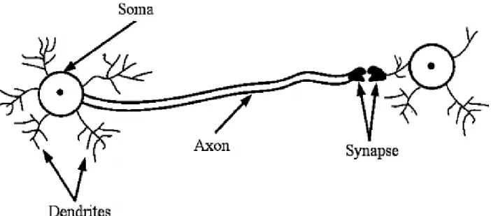
Artificial Neural Networks are inspired by biology multipolar neuron, which is one type of

neuron that consists an axon and many dendrites, working for integration of a large number of

information from other neurons. Figure 1 shows an example of biology neuron. Artificial neural

networks are based on the same concepts. They are grouped by particular layers. Figure 2 gives a

simple example. It totally has three layers, input layer, hidden layer and output layer, and each

layer has different number of neurons. Each neuron connects with all neurons of previous layer.

Every neuron of first layer receives input information. In the end, the output neurons extract all

information and create the output. Just like multipolar neurons, artificial neural network can do

some intelligence functions, like object recognition, tracking, classification and so on. The

(15)

4

person to get some new information. For example, a people learns to recognize a cat from examples

of cats. So in the testing step, ANNs can get the output that this is a cat or not.

Figure 2Artificial Neural Network

Convolutional Neural Network

Figure 3Left: Regular Artificial Neural Network. Right: Convolutional Neural Network[22]

Convolutional Neural Networks are a type of artificial neural networks with more complex

structure. The left of figure 3 shows the regular artificial neural network which has 4 layers and

(16)

5

becomes a high dimension array instead of a one column of neurons. The inputs of convolutional

neural networks are 2D dimensions such as images. Nowadays convolutional neural networks

achieve breakthrough on artificial intelligence area, such as computer vision, robotics, natural

language processing, big data analysis and so on.

Figure 4 Convolution computation illusion[22]

We already known the structure of convolutional neural network, so one question perhaps

comes up: how does convolutional neural network works. Figure 4 shows an example of

convolution operation in one layer. It has two important concepts, feature maps and kernel filters.

Feature maps are the output data from previous layer, so in the first layer its input data. Kernel

(17)

6

example, the column and rows are both 3. One feature map corresponds to one particular kernel

filter. Kernel filter does convolution operation with same size of feature map values, then it works

like a sliding window which slides by rows firstly and then by column to do convolution

computation with the whole feature map values. The values in the kernel filters care called weights.

One feature map shares one particular small size of weights. After finishing the whole processing

of all layers and creating the output, they still have a loss function such as SVM, Softmax

connected with the layer, which are used for backpropagation and can update the trainable weights.

In image classification perspective, the output values of last layer means the class scores.

Figure 5 An example of neuron computation[22]

The convolution layer is the most important layer in convolutional neural networks which

occupies the most part of the computation complexity. The output value of one kernel filter

convolution computation is the input of neuron of next layer. Suppose that the dimension of neuron

layer is N x N and the dimension of kernel filter is K x K. The size of the convolution layer output

(18)

7

𝑥

_𝑖𝑗𝑙

= ∑

𝑘−1_𝑎=0

∑

𝑘−1_𝑏=0

𝑤

_𝑎𝑏

𝑥

_{(𝑖+𝑎)(𝑗+𝑏)}𝑙−1

[ 1 ] In the equation, 𝑙 means the current layer numbers, and 𝑤 represents the weights of the kernel filter.

There is one important concept that need to be mentioned, hyperparameter. For example,

the number of input and output channels is a hyperparameter which also corresponds the size of

kernel filters. The stride of kernel filter to slides feature maps must be specified. Usually the stride

in convolutional neural network can be 1 or 2 and uncommonly 3 or more. If the stride is 2, the

kernel filters slides two rows or columns of the feature maps to do convolution operation. In

addition, sometimes the feature maps cannot slide completely if the stride is 2. In this situation,

we need to add padding to the feature maps and the values of the padding commonly is 0 which

has the minimum influence for the feature map information. The size of the zero-padding is also a

hyperparameter. There is an equation to help choose the suitable hyperparameters:

𝑁 = (W − K + 2P)/S + 1(W − K + 2P)/S + 1 [ 2 ] Where N means the number of neurons, W means the size of input feature maps, K represents the

size of kernel filter and S is the stride. For example, if the input feature maps size is 9 x 9, the size

of kernel is 3 x 3 with 1 stride and pad 0, the size of output feature maps should be 7 x 7.

Pooling layers use to shrink the size of feature maps which can reduce the computation

complexity and parameter size. Usually there are two types of pooling: max pooling and average

pooling. Max pooling computes the max value within the size of filter in the feature maps. Average

pooling is similar with max pooling, but compute the average value as the output. The most

common be used filter size is 2 x 2. Pooling layer just change the dimension of the feature map

(19)

8

Figure 6 An example of Pooling Layer [22]

Fully connected layers usuallyare connected after convolution layers. As shown in Figure

2. The “fully connected” means each neuron in current layer connects with every neuron in the previous layer. The activations can hence be computed with a matrix multiplication followed by a

bias offset. The biggest difference between fully connected layer and convolution layer is that

every feature maps in fc layer have own weights, however, one feature map in conv layer share a

kernel filter.

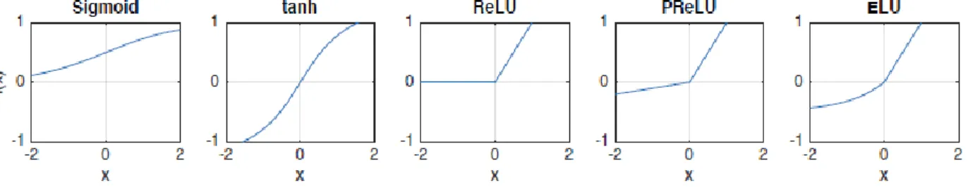
Convolutional neural network has different kinds of activation function.Activation function

is a mathematical function that be used to calculate the output of convolution computation in

current layer. Figure 6 shows 5 activation functions. Nowadays, ReLU perhaps the most popular

activation function. From the figure you can see that the ReLU is a max function which constraint

all negative inputs to zero and doesn’t change the positive one. Whatever forward and backward propagation, it is easy to do computation. It also can suffer less from vanishing gradient.

(20)

9

Figure 7 Activation Functions

Batch Norm layer works as a normalization that adjusts and scales the output of activation function. Figure 7 shows the algorithm of batch norm layer. Firstly, it subtracts the mini-batch means and then divides the mini-batch standard deviation. Batch Norm Layer. To

increase the stability of a neural network, batch normalization normalizes the output of a previous

activation layer by subtracting the batch mean and dividing by the batch standard deviation. Then

it adds two trainable parameters which will denormalize in the processing of backpropagation.

(21)

10

Binarized Neural Network

Figure 9 Binarized Neural Network Structure on CIFAR-10[4]

Binarized Neural Network[4] can be considered as extreme quantized version of convolutional neural network. Figure 7 shows binarized neural network structure on CIFAR-10 datasets which is based on VGG[21]. It has 6 convolutional layers, 3 max pooling layers and 3 fully connected layers. The most important difference between BNN and conventional CNN is that it uses binarized the activation and weights (i.e. +1, -1). The binarized weights function is a sign function:

𝑤𝑏 = 𝑆𝑖𝑔𝑛(𝑤) = {+1 𝑖𝑓 𝑤 ≥ 0

−1 𝑜𝑡ℎ𝑒𝑟𝑒𝑖𝑠𝑒 [ 3 ]

So the weights value in BNNs just two situation, –1 or +1. Except binarized the weights, it also binarized the activation function:

𝐹𝑜𝑟𝑤𝑎𝑟𝑑: 𝑞 = 𝑆𝑖𝑔𝑛(𝑟) = {+1 𝑖𝑓 𝑤 ≥ 0 −1 𝑜𝑡ℎ𝑒𝑟𝑤𝑖𝑠𝑒 [ 4 ] 𝐵𝑎𝑐𝑘𝑤𝑎𝑟𝑑: 𝜕𝑔 𝜕𝑟= { 𝜕𝑔 𝜕𝑞 𝑖𝑓 |𝑟| ≤ 1 0 𝑜𝑡ℎ𝑒𝑟𝑤𝑖𝑠𝑒 [ 5 ]

The binarized activation function is also sign function. The output of the activation function is -1 or +1. But there is a problem about activation backpropagation. Sign function is

(22)

11

not differential. So the BNN[4] propose a straight through estimator(STE) strategy to approximate the gradient for making binarization differentiable. From the equation above, if the absolute of binarized activation input is smaller than 1, then the gradient doesn’t change, otherwise, the gradient is equal to 0.

Figure 10 Sign Function

Field-Programmable Gate Arrays

This section will illustrate the high-level Field-Programmable Gate Arrays (FPGAs).

Firstly, I will introduce the basic concepts of FPGAs which includes the definition, structure and

application. Then, the high level synthesis will be mentioned. In the end, I will introduce existing

hardware platform for convolution neural network implementation and explain why I choose

(23)

12 Introduction

Figure 11 Basic FPGA Architecture [24]

From the name it’s straight forward that FPGAs consists of a huge number of gate arrays which are programmable. Figure 11 shows the basic structure of the FPFA. The first FPGA

introduced by Xilinx in 1985. It has lots of logic block which are connected by interconnect and

switch matrix unit. Logic block mainly consists of Look-up table (LUT) and flip-flop (FF). LUTs

are used for performs logic operations and FFs are used for store the results of LUTs. But with the

progress of times, FPGA is more complex nowadays. Some FPGAs has built-in other hardware

function such as DSP, faster communication interfaces, PCIe and so on. FPGAs are similar with

CPLDs, but FPGAs have larger size. There are mainly two FPGAs companies, Xilinx and Intel

FPGA(Altera). These two companies dominates around 90% of the FPGA market. One important

advantage of FPGA is reconfigurable and flexible. You can program it anytime and anywhere.

(24)

13

design FPGA project includes synthesis, netlist generation, routing and placement to create

bitstream file that FPGA can understand and run on it. Xilinx, Intel FPGA and other companies

has their own programming tools to do the whole processing such as Vivado and ISE. With the

high-level synthesis coming up, you also can program FPGA directly use high level language such

as C++, C, systemC and so on. I will introduce high level synthesis in the next section.

High-Level Synthesis

High-Level Synthesis (HLS) is an automated compiler that can synthesis high level

language like C/C++/SystemC to hardware description language like Verilog and VHDL, for

FPGA implementation. The high level codes can be architecturally constrain and synthesis

into a register-transfer level which can be further transfer to the grate level design for FPGA

implementation. High-Level Synthesis makes engineers efficiently and quickly design

hardware architecture and verify the hardware projects which saves the development cycle.

Vivado HLS is a popular High-Level Synthesis tool which is introduces by Xilinx

Company. Our work also use this software to design PC-BNN hardware inference architecture.

One disadvantage of high-level language is that it can not control the timing for the software

application. Vivado HLS use directive commands to constrain and optimize the design to

make it hardware-friendly. Using directive, we can define the interface and control the data

flow. It also can optimize the design. For example, loop unrolling directive can unroll the

specific loops and execute it in parallel. Loop and function pipelining can build a pipeline

(25)

14

block RAM resources. For example, data can be chosen to store in block Ram or Distributed

Ram. It can split one array to different dimensions and allocate different I/O ports.

Embedded Convolutional Neural Network Platform

GPUs have high throughput and performance, but also have huge energy consumption and

less energy efficiency. It can be developed quickly based on existing deep learning framework.

CPUs have less performance and power consumption than GPUs. It also has bad power

efficiency

AISCs can maximum energy efficiency, However, ASICs are even less suited for irregular

computation than FPGAs, are not suitable for model change and they need longer development

cycle.

FPGAs are well suited for BNN, as their dominant computations are bitwise logic

operations and their memory requirements are greatly reduced. FPGAs are reconfigurable to

customize different deep learning models. It has much less lower consumption. However,

(26)

15

CHAPTER THREE: PARALLEL-CONVOLUTION BINARY NEURAL

NETWORK

Figure 12 PC-BNN structure and accuracy

In this chapter, I will introduce our new Parallel-Convolution Binarized Neural Network

(PC-BNN) model. The Figure 12 shows the basic structure of the model. The most intuitive

difference with conventional BNN is that we replace the original binary convolution layer with

two parallel binary convolution layer. We will show later that such parallel convolution layer

design plays an important role in improving inference accuracy with limited model size increase

compared to conventional BNN. The PC-BNN model consists of one convolutional layer, five

convolutional blocks, two max pooling layer and one fully connected layer. We also uses fixed 3

x 3 kernel filters for all convolutional layers. As shown in Figure 12, I defined one Conv Block

which includes Batch Normalization, Binary Activation function (BinActive) and Binary

Convolution (BinConv) in parallel with additional cascaded Parametric ReLU (PReLU) layer. The

feature maps and weights are both binarized (i.e. +1, -1) in BNNs. From information theory

perspective, binarized neural networks have limited "knowledge" capacity which is not enough to

deal with large-scale challenge. Also, optimization with sign function itself is an open challenging

(27)

16

possible to find a good local optima. But for large-scale datasets, it's quite easy to fall into a bad

local optimization using SGD and that might be why the results on ImageNet dataset are not

promising. So, the accuracy of BNNs is greatly reduced. In order to extract more “information”,

we use two parallel convolution layers. Except the inputs to the first convolution layer (i.e. whole

network inputs) are real-value tensors, all the input tensors to the intermediate convolution layers

are binarized. The reason why we use two parallel layers instead of original one binarized

convolution layers but doesn’t choose 2bit or more fixed points bits to instead of binary format of

feature maps and weights is that binarized values of feature maps and weights can use xnor and

bitcount operation replaces dot product and accumulation in the convolution operation. The xnor

and bitcount operation are well suited for FPGA implementation which I will explain in detail in

the chapter 4. In addition, I also don’t choose to increase accuracy by expand the channels of feature maps. Because if the channels of feature maps increase by twice, the whole layer size will

increase 4x. Next I will introduce particular layers one by one.

(28)

17

Usually, the location of BatchNorm is between convolution layer and activation layer. In the

Figure 12 you can see that sequence of one Conv Block is BatchNorm-BinActive-BinConv-Max

pooling. There are mainly two reasons that we do this change:

1. BatchNorm plays a role in normalization and shift scaling the input of binarized activation

function, which could minimize the accuracy degradation.

2. BatchNorm prevents the input tensors of BinActive with patches of contiguous zeros that

will cause the accumulated information vanished.

In the table 2, C-B-A-P means Conv-BatchNorm-Activation-Pooling and B-A-C-P means

BatchNorm-Activation-Conv-Pooling. It shows that accuracy is increased when put BatchNorm

before the Activation function on XNOR net [1] which is one state-of-the-art BNN model on

ImageNet dataset.

Table 2 XNOR-Net two blocks structure comparison [1]

As discussion in chapter 2, I use the same binarized strategies to binarized (i.e. +1 and -1)

the input of convolution layer which add a binarized activation function before convolution layer.

In the forward propagation, the input tensors are binarized by Sign function. However, the sign

function has zero derivatives, which cannot calculate the gradient when do backward propagation.

(29)

18

the input gradient of binarized activation function are same with the gradient at output if the

absolute value is smaller than 1. Otherwise, the gradient is zero to preserve training processing.

Figure 13 Xnor and bitcount operation example

As been widely discussed in many recent works, scaling factor is the key factor to prevent

BNN from great reduction of inference accuracy. In our PC-BNN, for the intermediate BinConv

layers, the BatchNorm and PReLU layers play roles in element-wise scaling function which can

scale the input of the convolution layers. So, we don’t need to add weight scaling factor in every

convolution layers. In this case, the same binarization function with STE is used for all the

binarized convolution layers. Thus, the typical output scaling used in other BNN are not needed in

our work, which could totally eliminate the computation complexity. Since both the feature maps

and weights are binarized to -1 or +1, the original floating point Multiplication and Accumulation

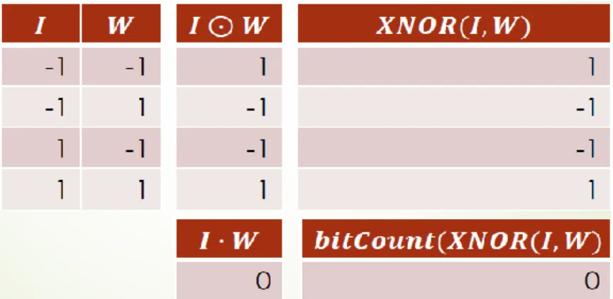
(MAC) operations in convolution layers can be replaces by xnorand bitcount, the figure 13 shows

an example how xnor and bitcount operation replace MAC computation. The mathematic

expression of xnor and bitcount operation is:

𝑋_𝑙𝑇∙ 𝑤𝑙= 2 × 𝑏𝑖𝑡𝑐𝑜𝑢𝑛𝑡(𝑥𝑛𝑜𝑟(𝑥𝑙, 𝑤𝑙)) − 𝑁; ∀𝑋𝐼,𝐿∈ [−1, +1] [ 6 ]

Where N presents the whole numbers of kernels to compute one output feature map, which is input

(30)

19

In this work, we implement PReLU as the activation function after the convolution layers,

which can further increase the accuracy. The figure 14 shows the curve of PReLU function. The

difference between PReLU and ReLU is that PReLU adds additional scaling influence for the input

tensors.

Figure 14 PReLU

The mathematic expression of PReLU is:

𝑓(𝑥) = { 𝑥 𝑖𝑓 𝑥 ≥ 0

𝑎𝑥 𝑜𝑡ℎ𝑒𝑟𝑤𝑖𝑠𝑒 [ 7 ]

Such function plays an important role of asymmetrical factor to scale the convolution output while

introducing more non-linearity. Moreover, since the dataflow between Conv-Blocks are in binary

format within such an ultra-compact neural network model, the conventional PeLU function

convert all negative input tensors to zero, which will cause more information loss in comparison

(31)

20

Figure 15 CIFAR-10 dataset [10]

We train our PC-BNN model on PyTorch framework. PyTorch is a Python-based scientific

package targeted at two sets of audiences, first, a replacement for NumPy to use the power of GPU,

second, a deep learning research platform that provides maximum flexibility and speed. We train

our model on CIFAR-10 dataset. CIFAR-10 dataset consists of 60000 images in 10 categories with

32 x 32 image size which has 600 images per class. 50000 images are used for training and the

rest 10000 images are used for testing.

In the training processing, we firstly go forward to binarized weights of every layer and get

the outputs. Then loss function to minimize the loss and change the trainable weights and our

model do inference at the same time using current weights. Thirdly, the original full precision

(32)

21

(33)

22

CHAPTER FOUR: FPGA ACCELERATOR DESIGN AND

IMPLEMENTATION

Introduction

PYNQ Platform Introduction

Figure 17 PYNQ Z1 Board

PYNQ stands for Python Productivity for Xilinx Zynq which is an open-source project that

makes it easy to design embedded systems with Xilinx Zynq® Systems on Chips (SoCs). It

consists of 650 MHz dual-core Cortex-A9 arm processor, Xilinx Artix-7 family FPGA board

which contains 13,300 logic slices, each with four 6-input LUTs and 8 flip-flops, 630 KB of fast

block RAM and 220 DSP slices, and 512MB DDR3 with 16-bit bus. The advantage of PYNQ

board is that people can directly use Python code to run PYNQ board even without use ASIC-style

design tools to design hardware architecture. The figure 18 shows the key technologies of PYNQ.

First people can use PYNQ IPs and PYNQ overlays to create bitstream file which FPGA can

understand. FPGA part of the PYNQ board are called programmable logic. Overlays are hardware

(34)

23

application programming interface (API). After creating the bitstream, we can write python

codes to run the bitstream by using API and the results can be shown on Jupyter Notebook.

Figure 18 PYNQ Design Flow

Data Type Consideration

In the training part, the inputs images are floating point. But FPGA are not good at

processing floating point operation. Because on CIFAR-10 dataset, all images are RGB format

which are 8bit. The range of pixels range from 0 to 255. So, in the FPGA implementation, the

input pixels are 8 bit fixed point. Except the input images, all the intermediate feature maps are

binary format. In this case, we can use xnor and bitcount operation to replace multiplication and

accumulation operation as mentioned before which can greatly reduce computation complexity

(35)

24 Motivation

The figure 19 shows the evolution of deep neural network. We can find that the models

become deeper and larger. They have enormous model size, massive computation cost and huge

energy consumption. For example, the VGG-19 network has 140 million floating-point parameters

and

Figure 19 Deep learning evolution

15 billion floating-point operations per image. The figure 20 shows that convolution layer occupy

most computation times. In this case, we consider to compression model size by using binarized

strategy which utilizing binarized convolution kernel can significantly reduce model size and

computation complexity. Convolution Operation of binary parameters (i.e.+1, -1) can be replaced

by xnor and bitcount operation, which paves a new road for energy–efficient FPGA

(36)

25

Figure 20 CNN computation time distribution

Overall Design Flow

Figure 21 Overall Design Flow

In this section, I will explain the whole design flow from PC-BNN training to FPGA

implementation. The hardware platform used is Xilinx Z1 board. This board is widely used in low

power embedded or mobile devices since its small energy consumption which at around 2.5W.

(37)

26

which brings a great challenge for conventional powerful neural network algorithm. Thus, the

main object of our hardware optimization is to reduce hardware resource usage while improving

throughput and energy efficiency of the system. First, we use PyTorch framework to train our

PC-BNN model. It can create a model file called “checkpoint.pth.tar” which contains all parameters. PyTorch[14] is a python package that provides tensor computation with strong GPU acceleration

and builds deep neural network on a tape-based autograd system. Note that, in this work, PC-BNN

model is trained on CIFAR-10 dataset [10], which is one of the most popular object classification

dataset. Then we extract the binarized network parameters from the ‘checkpoint.pth.tar’ file and

convert it to ’Parameter.bin’ which is used for neural network function software validation and FPGA mapping by PyTorch parameter extractor manually. Because the weights are full precision

in the ‘checkpoint.pth.tar’ file, we need to binarized the weights manually. In addition, another

important function of the extractor is to calculate the thresholds which are converted from

PReLU-BatchNorm-BinActive functions. I will explain it later in detail. Third, we start to design FPGA

PC-BNN inference architecture using two Xilinx Vivado softwares which are able to synthesis and

create the executable bitstream file that contains the network topology and can be understand by

PYNQ board. Finally, by using PYNQ API and overlay, it is easy to load bitstream file and

(38)

27

Overall Hardware Architecture

Figure 22 Overall Hardware Architecture

The figure 22 shows the overall hardware architecture. It is designed to be a streaming

pipeline structure. Ae, processor works as a controller to control the data communication between

off-chip memory and FPGA. AXI-Bus is one open standard for the connection and management

of functional blocks in a system-on-chip (SoC) which is responsible to communication between

off-chip and on-chip. In the on-chip (FPGA) part, there is block Ram unit which is on-chip memory

with 4.9 Mbit. Because our PC-BNN model totally has 2.3Mbit model size, so all the parameters

can be stored on on-chip memory which greatly reduce power consumption since communication

between on-chip and off-chip memory is extremely energy cost and time consuming and we don’t

need to communication between off-chip and on-chip for parameters transferring. As shown in

figure 14, there are totally 7 blocks which occupy hardware resources intendedly which

corresponding to every layer includes BinConv, Convblock and BinFC. It worth note that the

(39)

28

no floating-point MAC operations in every block. In addition, we use Xilinx HLS (high level

synthesis) data streaming mechanism to communicate between every block. The data streaming

works like a FIFO that reads and writes read in a sequence order which is well suited for our

pipeline architecture since it doesn’t need buffer to store intermediate data temporally. So, when

images data are loaded from off-chip memory to the first BinConv, the BinConv start to do

computation. Then when every block start to create the output data, the next block start to load

parameters from on-chip memory and do computation. The pipeline architecture can extremely

save computation time. In the end, the outputs of last layer are stored to off-chip memory. In the

whole processing, except load input images and store output to off-chip memory, the on-chip has

no communication with off-chip.

Hardware Optimization

In this section, I will discuss the hardware optimization strategies to design a

hardware-friendly FPGA architecture. Firstly, I will introduce hardware block design which change original

conv block. Then, I will illustrate how to convert PReLU-BatchNorm-BinActive functions to a

(40)

29

Hardware Block Design

Figure 23 Hardware Block Architecture

Previously one conv block is BatchNorm-BinActive-BinConv-PReLU. In order to more

efficiently map PC-BNN to FPGA, we relocated the conv block architecture to

BinConv-PReLU-BatchNorm-BinActive, which doesn’t change the whole streaming pipeline flow. Figure 23 shows

the hardware block architecture. The input of the previous convblock comes from previous PReLU

layer which are not binary value and the outputs of blocks are not binary value. So communication

between blocks are not efficiency. After changing the convblock sequence, the inputs of block

comes from precious BinActive are binary value and the output of blocks are also binary value.

There are mainly two benefits for this modification. Firstly, the inter-layer commutation data size

are greatly reduced which reduces the communication cost and easier to design the all convblocks

with the consistent interfaces. Secondly, it reduces the buffer that stores the transfer data which

save the hardware resources. In addition, this modification are well suited for our threshold unit

which are converted from PReLU-BarchNorm-BinActivation function because this modification

(41)

30

Converting PReLU-BatchNorm-BinActive to Threshold Function

BatchNorm actually is a complex equation and is very inefficient for FPGA

implementation. So, we consider how to optimize so that can avoid the computation. BatchNorm

can be considered as an affine function:

y = kx + b [7] Where: k = 𝛾 √𝛿2_{+ 𝜖} 𝑎𝑛𝑑 𝑏 = 𝛽 − 𝜇𝛾 √𝛿2_{+ 𝜖} [8]

Because BinActive is actually a sign function, the PReLU-BatchNorm-BinActive can be describes

as:

y = {𝑆𝑖𝑔𝑛(𝑘𝑥 + 𝑏) 𝑖𝑓 𝑥 ≥ 0

𝑆𝑖𝑔𝑛(𝑎𝑘𝑥 + 𝑏) 𝑜𝑡ℎ𝑒𝑟𝑤𝑖𝑠𝑒 [9]

We can translate the sign function with threshold value ∆, the equation above can be rewritten as:

y = {𝑆𝑖𝑔𝑛∆+(𝑥) 𝑖𝑓 𝑥 ≥ 0 𝑆𝑖𝑔𝑛∆₋(𝑥) 𝑜𝑡ℎ𝑒𝑟𝑤𝑖𝑠𝑒 [10] Where 𝑆𝑖𝑔𝑛∆₊(𝑥) = +1 and 𝑆𝑖𝑔𝑛∆₋(𝑥) = -1. ∆₊= −𝑏 𝑘 𝑎𝑛𝑑 ∆−= −𝑏 𝑎𝑘.

There are mainly two advantage after this transformation. Firstly, BatchNorm has complex

computation which is inefficient for FPGA implementation. We don’t need to do BatchNorm and

PReLU computation which are replaced by a simple comparison operation. It is greatly reduced

computation complexity. Secondly, we also don’t need to store and load BatchNorm parameters on on-chip memory. BatchNorm layer has two different parameters which is replaced by one

(42)

31

Processing Element

Figure 24 Processing Element

Figure 24 shows the detailed processing element architecture, which mainly consists of

three different units: XNOR units, popcount units and threshold units. As I mentioned before, the

inputs are outputs are streaming data format. It works as one dimension vector, so the data are

loaded to XNOR unit one by one. SIMD stands for single input multiple data and ‘s’ is the number

of data that are loaded. In the processing element, we convert the high dimension convolution

operation to matrix-vector computation. The parameters stored in BRAM also are loaded to XNOR

unit as a streaming flow which has the same bandwidth with input data. From the figure 16 you

can see that we have numbers of parallel XNOR unit. Each unit corresponds to one output channel

of feature maps, so every XNOR unit share the same input data and use different weights. The

processing element achieve input channel and output channel computation parallel and the

parallelism is flexible according to hardware resources. In every XNOR unit, input data do xnor

operation with correspond weights. In the popcount unit it popcount the output of xnor unit. After

(43)

32

the correspond threshold value. The processing element can be easily implemented to LUTs on

FPGA which are much energy efficient in comparison with conventional multiplication and

accumulation (MAC) computation and BatchNorm operation.

Sliding Window

Figure 25 Sliding Window

The original input data is 2D dimension. In order to get the right input streaming sequence

in the processing element, we need to reshape the dataflow using sliding window units. Since our

work is a streaming pipeline architecture and the size of the filter kernel is 3 x 3, we just need to

define a small size buffer to store input data. The height of the sliding window should be equal to

be the size of the filter kernel and the width of the sliding window equal to the width the of input

feature maps. As the convolution operation mechanism, the sliding window should load the data

that correspond to the kernel filter values one by one. In our work, it needs to send every 3 x 3 size

(44)

33

The size of sliding window is 3 x 3 and it will dynamically shift and load in sequentially. After it

finish sending the first 3 height input data, it will continue to load next 3 height input data. The

sliding window can greatly save FPGA resources because we don’t need to use buffer to store all

(45)

34

CHAPTER FIVE

：

EVALUATION AND RESULTS

Experimental Setup

As mentioned before, we use Xilinx PYNQ Z1 as the hardware platform. PYNQ Z1 is a

system on chip (SoC) which mainly consist of an XC7Z020 FPGA chip and dual-core ARM

Cortex-A9 embedded processor. The XC7Z020 is actually a small FPGA board which includes

53,200 LUTs, 106,400 FFs, 280 18Kb BRAMs, 220 DSP48Es. Take advantage of high-level

synthesis, we design our hardware architecture using C++ language by Vivado HLS software

which can synthesis the C++ codes to hardware language. And using Zynq IP in Vivado software

to create the bitstream file which is a bitfile that FPGA can understand. The images dataset is

CIFAR-10 [10] which as the test benchmark to do experiments.

Experimental Results

To better show our work, we compare our results with other three existing related works.

Table 3 lists the experimental results of all four works. These works have the same configuration.

They all implement binarized neural network to FPGA and use the same XC7Z020 FPGA board

and do inference on CIFAR-10 dataset. The original FINN use 200 MHz frequency. To better do

comparison, I reimplement this work to the XC7Z020 board and measure the results on 143 MHz

frequency. So all the four works have the same frequency. I will firstly introduce our experimental

results and then analysis the results in comparison with other works. In the table 3, it shows our

PC-BNN FPGA implementation consumes 13436 LUTs, 135 18K BRAMs, 53 DSP48E. As

(46)

35

to test the power since this board is charged by USB interface. We did 1000 images inference and

the power average to 2.4w for the whole board.

Table 3 Comparison with Other Binarized Implementation on the FPGA

Firstly, we compare our work with [18]. Although the [18] have 1.73% smaller test error

in comparison with our works, their model size is larger 11.1Mbits and the frame per second is

much higher than our work. Because our weight size is just 2.3 Mbit which can be all stored on

on-chip memory. The weight size of [18] is 13.4 Mbit. Since the on-chip memory is only 4.9 Mbits,

they have store partial parameters on off-chip memory and load parameters to FPGA in the whole

processing. The communication between off-chip and on-chip memory is much energy hungry, so

(47)

36

addition, the [18] reuses the intermediate feature map buffer, so they have to finish all computation

of current layer to start computation of next layer. However, our pipeline architecture can avoid

this issue. In the end, our PC-BNN model parameter size reduces by 5.8x, throughput (frame per

second, i.e. FPS) increases by 5.5x and frame per second/ watt is 14.5x better with only 1.71% test

error increased in comparison with this work.

Comparing our work with FINN[17], they also use the pipeline architecture. Our model is

more compact and efficient than them. The model of FINN[17] consists of six convolution layers,

three max pooling layers and three fully connected layers. But our work uses parallel convolution

layer structure and only one fully connected layer. The table 2 shows that FINN and our work

almost use the same number of LUTs. We achieves much higher accuracy and even have much

higher performance. Although we just use only one fully connected layers, the 4.9% test error

reduction demonstrates that our parallel convolution layer structure can efficiently extract more

image information.

Comparing our work with [12], they have the least parameter size, however, our frame per

second still higher than them. Because they store the parameters in the off-chip memory which has

higher communication latency to load parameters from off-chip to on-chip memory. In addition,

we still have 4.2% higher accuracy than this work. In summary, our work achieves ~86% accuracy

(48)

37

three works, we have the highest hardware efficiency and highest performance.

(49)

38

CHAPTER SIX

：

CONCLUSION

In this master thesis, we explore the FPGA implementation for binarized neural network

inference. We mainly have two contributions on software and hardware respectively. First, we

propose a new binarized neural network model, called Parallel-Convolution BNN (PC-BNN),

which replaces the original binary convolution layer in original BNN with two parallel binary

convolutional layer. Also, we only use one fully connected layer. Second, from the FPGA

implementation perspective, we relocated the block structure which makes dataflow more

hardware efficiently without changing the whole network model. We design a new processing

element unit which replaces the Multiplication and Accumulation operations with XNOR logic

and bitcount operations. It greatly reduces computation complexity and latency. Then, we convert

the PReLU-BinActive-Batchnorm functions to a threshold unit which uses a simple comparison

operation to replace the complex BatchNorm and PReLU operations. It further reduces the

computation requirement and saves memory usage. In the end, we design a streaming pipeline

architecture which stores all parameters on-chip and doesn’t need to communicate with off-chip

in the processing of intermediate layer. In summary, our PC-BNN model achieves 86% on

CIFAR-10 dataset with 2.3Mb parameter size. Compared with other three conventional BNN

implementations on the same Xilinx XC7Z020 board, our work has the best FPS and best accuracy

(50)

39

LIST OF REFERENCES

1. Rastegari, M., Ordonez, V., Redmon, J. and Farhadi, A., 2016, October. Xnor-net:

Imagenet classification using binary convolutional neural networks. In European

Conference on Computer Vision (pp. 525-542). Springer, Cham

2. Yoshua Bengio et al. 2013. Estimating or propagating gradients through stochastic

neurons for conditional computation. arXiv preprint arXiv:1308.3432 (2013).

3. Matthieu Courbariaux et al. 2015. Binaryconnect: Training deep neural networks with

binary weights during propagations. In Advances in neural informationprocessing

systems. 3123–3131.

4. Matthieu Courbariaux et al. 2016. Binarized neural networks: Training deep neural

networks with weights and activations constrained to+ 1 or-1. arXivpreprint

arXiv:1602.02830 (2016).

5. Song Han et al. 2015. Deep compression: Compressing deep neural networks with

pruning, trained quantization and huffman coding. arXiv preprintarXiv:1510.00149

(2015).

6. Kaiming He et al. 2016. Deep residual learning for image recognition. In Proceedings of

the IEEE conference on computer vision and pattern recognition. 770–778.

7. Sergey Ioffe et al. 2015. Batch normalization: Accelerating deep network training by

reducing internal covariate shift. In International conference on machinelearning. 448–

(51)

40

8. Juefei-Xu, F., Boddeti, V.N. and Savvides, M., 2017, July. Local binary convolutional

neural networks. In Computer Vision and Pattern Recognition (CVPR), 2017 IEEE

Conference on (Vol. 1). IEEE.

9. Krizhevsky, A., Sutskever, I. and Hinton, G.E., 2012. Imagenet classification with deep

convolutional neural networks. In Advances in neural information processing

systems (pp. 1097-1105).

10. Alex Krizhevsky et al. 2014. The CIFAR-10 dataset. online: http://www. cs. toronto.

edu/kriz/cifar. html (2014).

11.Lin, X., Zhao, C. and Pan, W., 2017. Towards accurate binary convolutional neural

network. In Advances in Neural Information Processing Systems (pp. 345-353).

12.Hiroki Nakahara et al. 2017. A fully connected layer elimination for a binarizec

convolutional neural network on an FPGA. In Field Programmable Logic and

Applications (FPL),2017 27th International Conference on. IEEE, 1–4.

13.Netzer, Y., Wang, T., Coates, A., Bissacco, A., Wu, B. and Ng, A.Y., 2011, December.

Reading digits in natural images with unsupervised feature learning. In NIPS workshop

on deep learning and unsupervised feature learning (Vol. 2011, No. 2, p. 5).

14.Adam Paszke et al. 2017. Pytorch. (2017).

15. Sung, W., Shin, S. and Hwang, K., 2015. Resiliency of deep neural networks under

quantization. arXiv preprint arXiv:1511.06488

16.Tang, W., Hua, G. and Wang, L., 2017, February. How to train a compact binary neural

(52)

41

17.Yaman Umuroglu et al. 2017. Finn: A framework for fast, scalable binarized neural

network inference. In Proceedings of the 2017 ACM/SIGDA InternationalSymposium on

Field-Programmable Gate Arrays. ACM, 65–74.

18.Ritchie Zhao et al. 2017. Accelerating binarized convolutional neural networks with

software-programmable fpgas. In FPGA. ACM, 15–24.

19.Shuchang Zhou et al. 2016. DoReFa-Net: Training low bitwidth convolutional neural

networks with low bitwidth gradients. arXiv preprint arXiv:1606.06160 (2016).

20.Ioffe, Sergey, and Christian Szegedy. "Batch normalization: Accelerating deep network

training by reducing internal covariate shift." arXiv preprint arXiv:1502.03167 (2015). 21.Simonyan, Karen, and Andrew Zisserman. "Very deep convolutional networks for

large-scale image recognition." arXiv preprint arXiv:1409.1556 (2014).

22.http://cs231n.github.io/convolutional-networks/

23.He, Zhezhi, Boqing Gong, and Deliang Fan. "Optimize Deep Convolutional Neural

Network with Ternarized Weights and High Accuracy." arXiv preprint

arXiv:1807.07948 (2018).

24.http://www.ee.columbia.edu/~kinget/EE6350_S16/04_FPGA_Tom_Robert_Harrison_Gu