Bed Drag Coefficient Variability under Wind Waves in a Tidal Estuary

Bed Drag Coefficient Variability under Wind Waves

in a Tidal Estuary

Jeremy D. Bricker

; Satoshi Inagaki

; and Stephen G. Monismith, A.M.ASCE

Abstract:In this paper we report the results of a study of the variation of shear stress and the bottom drag coefficient CDwith sea state

and currents at a shallow site in San Francisco Bay. We compare shear stresses calculated from turbulent velocity measurements with the model of Styles and Glenn reported in 2000. Although this model was formulated to predict shear stress under ocean swell on the continental shelf, results from our experiments show that it accurately predicts these bottom stress under wind waves in an estuary. Higher up in the water column, the steady wind-driven boundary layer at the free surface overlaps with the steady bottom boundary layer. By calculating the wind stress at the surface and assuming a linear variation of shear between the bed and surface, however, the model can be extended to predict water column shear stresses that agree well with data. Despite the fidelity of the model, an examination of the observed stresses deduced using different wave–turbulence decomposition schemes suggests that wave–turbulence interactions are im-portant, enhancing turbulent shear stresses at wave frequencies.

DOI:10.1061/共ASCE兲0733-9429共2005兲131:6共497兲

CE Database subject headings:Drag coefficient; Hydraulic roughness; Turbulence; Tidal currents; Waves; Estuaries.

Introduction

The erosion, transport, and deposition of sediments play a central role in many geological, biological, geochemical, and ecological processes operant in estuaries共Shrestha and Orlob 1996兲. Accord-ingly, engineering studies done to assess how large-scale works such as constructing airport runways on new landfill, restoring tidal wetlands, or changes in the disposal of dredge materials might degrade or improve the environment of the estuary on which these actions would take place often make use of coupled hydrodynamic/sediment transport models that are designed to pre-dict sediment dynamics共Blumberg et al. 1999兲. A key feature of all these models is the way in which bed friction is modeled, i.e., how it depends on bed roughness, mean currents, and as we dis-cuss in this paper, how it is affected by wind-wave orbital mo-tions共Perlin and Kit 2002兲.

In most three-dimensional 共3D兲 circulation models, bottom friction is represented by a quadratic drag law based on a bottom drag coefficient CD

␶c=␳CD兩Uc兩Uc 共1兲

where ␶c= steady shear stress at the bed; ␳= water density; and Uc= velocity of the mean current at height zr共Signell et al. 1990兲,

usually taken as 1 m above the bed共mab兲. In 3D modeling,␶cis

then used as a bottom boundary condition on the velocity. ␶c= −␳␯c

⳵U

⳵z 共2兲

where␯c= eddy viscosity.

It is commonly assumed, and often found to be true in practice

共Nezu and Nakagawa 1993; Lueck and Lu 1997兲, that the well-known law of the wall 共e.g., Tennekes and Lumley 1972; Nezu and Rodi 1986兲 兩Uc兩= 兩u*c兩 ␬ ln

冉

冊

the bed共Nikuradse 1932兲; and the shear velocity is u*c=

冑

␶c

␳ 共4兲

Using these relations, CD, referenced to some height zr, can be

inferred from the roughness length CD=

冋

␬ ln共zr/z0兲

册

2

共5兲

关see, e.g., Gross et al. 1999兴. Generally, the value of CDdepends

upon bed sediment grain size and bed-form geometry.

However, in the shoals of many estuaries, areas that are often of particular environmental and engineering concern, currents and sediment dynamics can be strongly influenced by wind waves

共Schoellhammer 1996兲. As discussed by Grant and Madsen

共1979兲and others共e.g., Fredsøe 1984; Perlin and Kit 2002兲,

bot-1

Research Associate, Dept. of Civil Engineering, Kobe Univ., 1-1 Rokkodai-cho, Nada-ku, Kobe 657-8501, Japan. E-mail: bricker@ stanfordalumni.org

2

Senior Research Engineer, Environmental Engineering Dept., Kajima Technical Research Institute, 2-19-1, Tobitakyu, Chofu-shi, Tokyo 182-0036, Japan. E-mail: [email protected]

3_{Professor, Environmental Fluid Mechanics and Hydrology, Dept. of}

Civil and Environmental Engineering, Stanford Univ., Stanford, CA 94305-4020. E-mail: [email protected]

Note. Discussion open until November 1, 2005. Separate discussions must be submitted for individual papers. To extend the closing date by one month, a written request must be filed with the ASCE Managing Editor. The manuscript for this paper was submitted for review and pos-sible publication on March 4, 2003; approved on September 13, 2004. This paper is part of the Journal of Hydraulic Engineering, Vol. 131, No. 6, June 1, 2005. ©ASCE, ISSN 0733-9429/2005/6-497–508/$25.00.

tom drag is enhanced when surface waves are long enough to reach the bed. In this case, a thin, oscillatory, wave boundary layer关also known as a Stokes layer共Kundu 1990兲兴develops near the bed that is more strongly sheared and experiences phase-dependent stresses that are larger than those operant in the thicker, steady current bottom boundary layer. It is the rectification of the periodic stress that alters the overlying flow.

Grant and Madsen 共1979兲modeled the inner wave boundary layer using an eddy viscosity based on a phase-dependent shear velocity, u*cw, defined by the phase-dependent bottom stress 共which is due to both waves and currents兲to determine velocity structure. Outside the wave layer, Grant and Madsen determine the effect of this inner wave layer on the main part of the bound-ary layer by requiring the outer flow stress and velocity to match the time averaged stresses and velocities of the inner wavy flow. The result is that enhanced turbulence within the wave layer re-sults in greater drag on the mean flow, an effect that can be modeled as an enhanced apparent roughness. The original Grant– Madsen model has been extended by various writers, most re-cently Styles and Glenn共2000, hereinafter SG2000兲, who incor-porated the effects of stratification as well as adjusting the assumed profile of eddy viscosity upon which the theory is based. Fredsøe’s共1984兲model is similar to that of Grant and Madsen, although he assumed logarithmic profiles rather than solving ex-plicitly for the velocity structure. At the other end of the spec-trum, Perlin and Kit 共2002兲 make no assumptions about eddy viscosity profiles, instead using a turbulence closure that solves for the phase-dependent turbulent kinetic energy 共TKE兲 from which phase-dependent eddy viscosities, etc. can be computed. In a similar fashion, Groeneweg and Klopman共1998兲more formally evaluated the average effects of waves on mean currents using a K-␧model and generalized Lagrangian mean共GLM兲averaging.

Most circulation models use a drag coefficient to parameterize bottom drag 共e.g., Casulli and Cattani 1994; Blumberg et al. 1999; Gross et al. 1999兲. Since these models resolve neither in-dividual waves nor the thin wave bottom boundary layer, the effects of waves are then included via a wave-dependent CDor

wave-dependent roughness 共Davies and Lawrence 1994, 1995; Signell and List 1997; Xing and Davies 2003兲. Kagan et al.

共2003兲found that inclusion of ocean-swell-enhanced roughness in a circulation model of Cadiz Bay brought tidal stage and currents predicted by the model into better agreement with observations. All of these studies have found that wave-enhanced roughness can have significant effects on tidal and wind-driven circulation, flushing rates and residence times of contaminants, channel-shoal asymmetry, and sediment transport.

Despite the recent application of Grant and Madsen’s en-hanced roughness theory to a variety of circulation models, field experiments to test the validity of this theory have been carried out only under ocean swell on the continental shelf共Cacchione et al. 1994; Drake and Cacchione 1992; Green and McCave 1995; Lacy et al., unpublished兲, and not under wind waves on the shoals of an estuary. For ocean swell on the continental shelf, the steady surface wind-driven boundary layer and the steady current bottom boundary layer are separated by an inviscid core共Grant and Mad-sen 1986兲; these are the conditions for which Grant and Madsen’s model was formulated. The accuracy of the drag coefficients and stresses predicted by models like that of Grant and Madsen have not been tested for shallow flows on the shoals of an estuary in the presence of wind waves, an environment where these two steady boundary layers overlap.

In this paper we investigate the variation of shear stress and CDunder combined tidal currents and wind waves共generated by

the local diurnal sea breeze兲on a shoal in South San Francisco Bay. Our results show that the model presented by Styles and Glenn 共2000, hereinafter SG2000兲, while formulated for ocean swell on the continental shelf, is capable of reasonably accurate predictions of the enhancement of shear stress and the bed drag coefficient over estuarine shoals by wind waves.

Experiments

To investigate variations of water column shear stresses and the bed drag coefficient under wind waves on the shoals of a tidal estuary, we ran two experiments at Coyote Point in South San Francisco Bay共SSFB, Fig. 1兲. This location was chosen because of ease of access and because of an interest in understanding circulation and sediment processes in this part of the SSFB in light of proposals to build new runways nearby on fill that would be placed on the local shoals. Our experiments took place in June of 2000 and June-July of 2002. Each experiment was run for 2 weeks to capture a full spring-neap tidal cycle. Coyote Point experiences mixed semidiurnal/diurnal tides, a diurnal sea breeze

共in summer兲, and frequent spilling whitecaps. The bathymetry at the study site is relatively flat, with a depth varying between 1 and 4 m during a near-solstice spring tide. The bed at the study site consists of silts and fine sands 共a representative value of kb

= 0.01 cm兲, and bed forms were not present. Shoreward共south兲of the site is a gently sloping sandy beach, which causes incident waves to break as spilling and plunging breakers, and prevents reflections.

Instruments

During the first共June 2000兲experiment we deployed two SonTek field acoustic Doppler velocimeters 共ADVs兲mounted on a mast sitting approximately 90 m north of the beach at high water共see Figs. 1 and 2兲 and in 1 m of water 共mllw—mean lower low water兲. The ADV measuring volumes were located 20 and 62 mab共centimeters above bed兲. These instruments sampled three components of velocity at 25 Hz, had an accuracy of ±3 mm/ s, and were cabled to computers on the shore for data acquisition. Approximately 200 m further north共and thus further offshore兲we deployed an upward-looking 1.5 MHz NorTek high-resolution acoustic Doppler profiler 共ADP兲 mounted on a small gimbaled frame. Operating in a pulse-to-pulse-coherent mode共Lohrman et al. 1990兲, it recorded 2-min averages of all three components of velocity in 3 cm bins covering a range of depths from 43 to 133 cmab. Time-averaged measurements of tidal stage and sea state were made with a SeaBird SBE26 absolute pressure sensor共accuracy greater than 1 mm in free surface elevation兲. An Ocean Sensors OS200 CTD made conductivity and temperature measurements. To record local wind speed and direction, we mounted an anemometer on a 3 m high mast. However, because the shore site where the anemometer was deployed was partially shielded by trees, for our analysis below we used an average of local winds as measured by the anemometer and those recorded nearby at San Francisco International Airport 共SFO兲, located about 2 mi upwind共northwest兲of the study site.

During the second experiment 共June-July 2002兲 we made a more comprehensive set of measurements: Along with 3 SonTek ADVs measuring velocities at 20, 53, and 153 cmab we also de-ployed a NorTek Vector ADV measuring velocities at 95 cmab. In addition to the SBE26 used previously, we also used a capacitive wave gauge共1 cm accuracy; 1 mm precision兲to measure surface

waves. For wave–turbulence decomposition purposes 共see below兲, the wave gauge was synchronized with the ADVs. In order to get a more complete velocity profile than we had in 2000, the body of the ADP was buried, so the transducer face was nearly flush with the bed, giving us good data starting at 15 cmab and extending to a maximum of 200 cmab共at high tide兲. Finally, in addition to the OS200 CTD, temperature was also measured by a vertical array of six high-precision 共±0.01° C兲SeaBird SBE39 temperature loggers. Unfortunately, during the second experiment our anemometer failed and so when needed for analysis, we used wind data from San Francisco International Airport’s 共SFO兲 weather station.

Observations of Conditions at Coyote Point

During both experiments, winds were nearly westerly in direction and diurnal in strength, reaching 12 m / s each afternoon 关Fig. 3共a兲兴which corresponds to a stress of approximately 0.2 Pa关Fig. 3共b兲兴. Waves showed the same diurnal trend, increasing to a maxi-mum height H_s= 50 cm and a period, T_w= 2 s in the afternoon

关Figs. 3共c and d兲兴. These periods and amplitudes are in good agreement with what might be predicted using formulas presented in the U.S. Army Corps of Engineers Shore Protection Manual

共Bricker 2003兲.

Tidal velocities reached a maximum of 30 cm/ s during peak flood with a favorable wind关Fig. 4共a兲兴. Flood currents were stron-ger than ebb currents共maximum ebb velocity was about 5 cm/ s兲, and flood usually lasted longer than ebb, due to both the

topog-raphy of the site and the winds over the site. Due to local bathym-etry, the flood tide共coming from the north兲hit the study site on the north side of Coyote Point with full force, while during ebb tide, the study site was in the lee of the Point, and was thus in its wake. During the afternoons, near-bed wainduced orbital ve-locities averaged 12 cm/ s, and was thus comparable in strength to the tidal current although they were nearly orthogonal to the tidal current关Fig. 4共b兲兴. Bottom stresses共determined as below兲ranged from 0 to 0.13 Pa.

Fig. 2.Schematic of instrument arrangement共see text for details兲 Fig. 1.Coyote Point共South San Francisco Bay, Calif.兲field site

Fig. 3. Conditions existing in June 2002: 共a兲 wind speed at 10 m measured at San Francisco International airport 共SFO兲; 共b兲 wind stress calculated per Eq.共11兲from the SFO winds;共c兲significant wave height at the instrument array;共d兲dominant wave period at the instrument array; and共e兲tidal variations in water depth at the instrument array

Fig. 4.Velocities and stresses measured in June 2002 by ADV located at z = 20 cmab:共a兲long-shore共—兲and cross-shore共--兲mean velocity;共b兲 long-shore 共—兲 and cross-shore共--兲 wave orbital velocity; and共c兲 long-shore turbulent shear stress inferred by the phase method共…兲, the Benilov–Filyushkin method共—兲, and by the Shaw–Trowbridge method共-.兲

Analysis Methods

Determination of Shear Stress via Time Series of Point Velocity Measurements

In principle, turbulence data from the vertical array of ADVs can be used to determine CD by assuming a constant-stress steady

bottom boundary layer and directly calculating Reynolds stresses from the fluctuating velocities. However, because variance asso-ciated with the waves is much larger than that assoasso-ciated with turbulence, some form of wave–turbulence decomposition scheme must be used共Jiang and Street 1991; Thais and Magnau-det 1995; Trowbridge 1998兲. As we will discuss below several approaches are possible and it remains an open question as to which is most appropriate in a given situation.

In a flow with both waves and currents, the instantaneous ve-locity can be written as

u = U + u˜ + u⬘ 共6兲

where U = mean velocity; u˜ = wave velocity; and u⬘= turbulent ve-locity. After Reynolds averaging the mean momentum equation using Eq. 共6兲, the Reynolds stress becomes关see, e.g., Jiang and Street共1991兲兴

−␶

␳= u˜w˜ + u˜w⬘+ u⬘w˜ + u⬘w⬘ 共7兲 For irrotational waves共Dean and Dalrymple 1991兲, the first term on the right-hand side 共RHS兲 of Eq. 共7兲 is zero. Furthermore, when waves and turbulence coexist, the latter can be defined as motions that do not correlate with waves共Jiang and Street 1991; Thais and Magnaudet 1995兲, so the second and third terms on the RHS of Eq.共7兲are also zero. Thus, under these conditions, the Reynolds stress is the same as that which is found for steady flows

−␶

␳= u⬘w⬘ 共8兲

As shown by Trowbridge 共1998兲, small uncertainties in instru-ment orientation or a gently sloping bed can bias velocity mea-surements such that in practice u˜w˜ may not be exactly zero.

In analyzing our data, we used three methods of wave– turbulence decomposition to remove the waves from our turbu-lence data. The first was that of Benilov and Filyushkin共1970兲, in which motions that correlate with displacement of the free surface are considered to be due to the waves. The second was that of Trowbridge共1998兲; and Shaw and Trowbridge共2001兲, which uses two velocity measurements spaced farther apart than the largest turbulence scale关approximately 1₄ the water depth, according to Shaw and Trowbridge 共2001兲兴, but are well within one surface wave wavelength of each other. Motions that correlate between the sensors are waves, while motions that are uncorrelated are defined as turbulence. The third method, which we call the “Phase Lag” method, is described in Bricker共2003兲. Assuming equilib-rium turbulence and no wave–turbulence interaction, in this method the phase lag between the u and w components of surface waves is used to interpolate the magnitude of turbulence under the wave peak within the inertial subrange of the spectral domain, which is otherwise removed. In essence, in this approach, one removes not only the waves, but also the local enhancement of turbulence at or near wave frequencies共see Lumley and Terray 1983兲.

After applying the various wave decompositions, we calcu-lated u⬘w⬘ using blocks of 213_{samples 共about 5}1

2 min of data兲. This period was chosen because it is significantly longer than the wave period, yet shorter than the time over which the sea state or tidal regime would change. We assumed that the lowest ADV共z = 20 cmab兲 measurements came from within the constant-stress inner layer of the steady bottom boundary, and thus that values of u⬘w⬘measured there are equivalent to the bottom stress exerted on the mean current. Lastly, using this value of u⬘w⬘, CDcan be

found in the usual fashion from Eqs.共1兲and共8兲.

Determination of Theoretical Shear Stress via SG2000 and the Overlap Method

Shear stress was also calculated at the bed via SG2000, which assumes bottom-boundary-layer turbulence only. Stress was then calculated at the height of each ADV via the overlap method共see below兲, which takes into account the wind-driven surface bound-ary layer. To use SG2000, we needed to supply the model with the following inputs:␾c, the angle between waves and the mean

cur-rent; Uc, a reference current a height zrabove the bed; uband Ab,

the near-bottom wave orbital velocity and excursion, respectively; and kb, the physical roughness scale. The reference height zrwas

taken as the height above the bed of each ADV. The other input parameters were determined via the methods below.

Fine-grain sand dominates the near-shore subtidal zone at Coyote Point. For typical values of u*at Coyote Point, a physical roughness of kb= 0.01 cm, appropriate for fine sand, means that

the flow was hydraulically smooth. As a result, the equivalent z0 for a hydraulically smooth bed is z0= 0.11␯/ u*c, resulting in z0 = 0.001 cm. Rather than use a variable value of z0, we used this constant value of z0as an input to SG2000.

Maximum wave-induced near-bed orbital velocity u_b, orbital excursion Ab, and the angle between waves and currents␾cwere

determined spectrally from linear wave theory 共Dean and Dal-rymple 1991兲using ADV and SBE26 data. With all these param-eters determined, SG2000 then calculated the steady shear stress near the bed, and Eq. 共1兲was used to determine the drag coeffi-cient based on this shear stress.

Overlap with Surface Wind-Driven Layer—The Overlap Method

Since the wind-driven surface boundary layer can overlap the bottom boundary layer in shallow flows, we further modified the approach given by SG2000 by assuming a linear variation in stress between the bed and the surface. Neglecting nonlinear ac-celerations and assuming pressure to be hydrostatic, the mean momentum equation in the x direction is

⳵U ⳵t = − g ⳵␩ ⳵x + 1 ␳ ⳵␶ ⳵z 共9兲

where␩= free surface deflection. The pressure term has no depth dependence, and the unsteady term is observed to vary far more with time than with depth共Fig. 5兲. Therefore, to a first approxi-mation

⳵␶

⳵z= f共t兲 共10兲

i.e., we can make the approximation that stress varies linearly with depth. From a practical standpoint, a linear variation is the

most complex one we can predict, given knowledge only of stresses at the bed and the surface.

Each component of the wind stress at the surface takes the form

␶wind=␳airCD,windU10

2 _共11兲

resulting in a shear velocity at the top of the water column of

u*wind=

冑

with C_D,winddetermined from Yelland and Taylor’s共1996兲 empiri-cal relations. The stress throughout the water column was then assumed to vary linearly from its共vector兲value at the bed共u*c兲to its 共vector兲value at the surface共u*wind兲. Finally, in our “overlap method,” the predicted stress at the height of each ADV is calcu-lated using a linear interpolation between the calcucalcu-lated bottom stress and calculated surface stress.

Discussion

Effect of Waves on Bottom Stress

In what follows, we assume that the observed stresses are best represented by stresses determined via the phase method. In Fig. 6 we plot the June 2002 data; the June 2000 data is essentially identical and is not shown. We note that near bottom stresses calculated via Shaw and Trowbridge’s method 关Fig. 6共a兲兴 agree well with those calculated by the phase method. We also note that because the surface stress has little effect on the stress near the bottom, predictions of the bottom stress made using only SG2000 are essentially identical to those made using the more complete overlap method 关Figs. 6共b and c兲兴. In general either prediction based on SG2000 gives a reasonable prediction of the effects of waves on bottom stress. However, by comparison, the constant C_Dcase, at least if based on a physically plausible value of C_D, consistently underestimates the stress. Clearly, in terms of use in a numerical model for cases where winds and hence waves are Fig. 5. Acceleration measured by the ADP in June 2002 at z

= 100 cmab as a function of the acceleration at z = 60 cmab. The line shown marks the case where the two accelerations are equal.

Fig. 6.Stresses at 20 cmab in June 2002 as functions of stresses inferred using the phase lag method共“Phase”兲:共a兲stresses inferred from ADV data using the Shaw and Trowbridge method共“ST”兲;共b兲stresses computed from wave and mean flow conditions using the model of Styles and Glenn共“SG”兲;共c兲stresses computed from wave and mean flows using the overlap method based on Styles and Glenn and a linear variation of stress over depth; and共d兲stresses computed using a constant value of C_Dand measured mean currents

relatively repeatable 共for example, in the case of diurnal sea breezes兲, CDcould be adjusted upwards in the calibration process

to match observation as was done by, e.g., Gross et al.共1999兲. The difference between the constant CDcase and the

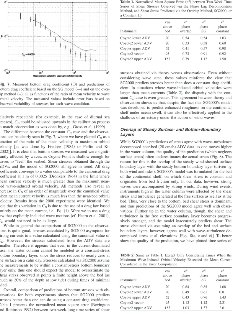
observa-tions can be clearly seen in Fig. 7, where we have plotted CDas a

function of the ratio of the mean velocity to maximum orbital velocity 关as was done by Fredsøe 共1984兲 or Perlin and Kit

共2002兲兴. It is clear that bottom stresses we measured were signifi-cantly affected by waves, as Coyote Point is shallow enough for waves to “feel” the seabed. Shear stresses obtained through the ADVs, and the model of SG2000, all agree in trend. All drag coefficients converge to a value comparable to the canonical drag coefficient at 1 m of 0.0025共Dronkers 1964兲in the limit where mean current velocity is much greater than the maximum near-bed wave-induced orbital velocity. All methods also reveal an increase in CDof an order of magnitude over the canonical value

when mean current velocity is much less than the near-bed orbital velocity. Results from the 2000 experiment were identical. We note that this variation in CDis due to the use of a drag law based

entirely on the mean current, i.e., Eq.共1兲. Were we to use a drag law that explicitly included wave motions共cf. Hearn et al. 2001兲, CDwould not need to be as large.

While in general the comparison of SG2000 to the observa-tions is quite good, stresses calculated by SG2000 asymptote for strong currents to a value calculated using the canonical value of CD. However, the stresses calculated from the ADV data are

smaller. Therefore it appears that even in the current-dominated case, the water column cannot be modeled as a constant-stress bottom boundary layer, since the stress reduces to nearly zero at the surface on a calm day. Stresses calculated via SG2000 assume the measurements to be within a constant-stress bottom boundary layer only, thus one should expect the model to overestimate the shear stress observed at points a finite height above the bed 共as much as 20% of the depth at low tide兲during times of minimal wind.

Overall, comparison of predictions of bottom stresses with ob-servations for both experiments shows that SG2000 predicts stresses better than one can do using a constant drag coefficient. Table 1 presents the normalized mean square error 共Bevington and Robinson 1992兲between two-week-long time series of shear

stresses obtained via theory versus observations. Even without considering wave state, these values reinforce the view that SG2000 predicts stresses better than does a constant drag coeffi-cient. In situations where wave-induced orbital velocities were larger than mean currents 共Table 2兲, the disparity with the con-stant C_Dcase is even greater. This agreement between theory and observation shows us that, despite the fact that SG2000’s model was developed to predict enhanced roughness on the continental shelf under ocean swell, it can also be effectively applied to the shallows of an estuary under the action of wind waves.

Overlap of Steady Surface- and Bottom-Boundary Layers

While SG2000’s predictions of stress agree with wave–turbulence decomposed near-bed共20 cmab兲ADV data, as one moves higher in the water column, the quality of the prediction共which neglects surface stress兲often underestimates the actual stress共Fig. 8兲. The reason for this is the overlap of the steady wind-sheared surface boundary layer with the steady bottom boundary layer共driven by both wind and tides兲. SG2000’s model was formulated for the bed of the continental shelf, on which shear stress is constant and originates from bed friction only. In our data, however, strong waves were accompanied by strong winds. During wind events, instruments high in the water column were affected by the shear stress and turbulence generated at the free surface as well as at the bed. Thus, very close to the bottom, bed shear stress is dominant, and thus predictions of the SG2000 model agree well with obser-vations. Further up in the water column, though, the shear and turbulence in the free surface boundary layer becomes progres-sively stronger, and the model inaccurately predicts shear. The stress obtained via assuming an overlap of the bed and surface boundary layers, however, agrees well with wave–turbulence de-composed stress at all elevations关Figs. 8共a, c and e兲兴. To better show the quality of the prediction, we have plotted time series of Fig. 7. Measured bottom drag coefficient 共䊊兲 and predictions of

bottom drag coefficient based on the SG model共—兲and on the over-lap method共--兲, all as functions of the ratio of mean velocity to wave orbital velocity. The measured values include error bars based on observed variability of stresses for each wave condition.

Table 1.Normalized Mean Square Error共␧2_{兲between Two-Week Time}

Series of Shear Stresses Observed via the Phase Lag Decomposition Method, and Shear Stress Predicted via the Overlap Method, SG2000, or a Constant CD Instrument cm above bed ␧2 phase overlap ␧2 phase SG ␧2 phase constant

Coyote lower ADV 20 0.54 0.54 1.03

Coyote2 lower ADV 20 0.33 0.38 0.60

Coyote upper ADV 62 0.41 0.57 0.98

Coyote2 vector 95 0.73 0.91 0.92

Coyote2 upper ADV 153 0.79 1.12 1.50

Table 2. Same as Table 1, Except Only Considering Times When the Maximum Wave-Induced Orbital Velocity Exceeded the Mean Current Considered in the Error Computation

Instrument cm above bed ␧2 phase overlap ␧2 phase SG ␧2 phase constant

Coyote lower ADV 20 0.84 0.85 1.68

Coyote2 lower ADV 20 0.49 0.61 0.81

Coyote upper ADV 62 0.43 0.76 1.43

Coyote2 vector 95 1.13 1.12 2.31

the stresses at 153, 95, and 20 cmab from the 2002 experiment along with the corresponding predictions of the overlap method based on SG2000 共Fig. 9兲. Excepting spikes in the observed stresses, most likely associated with instrument noise, the overall agreement is excellent, lending support to the conclusion that the SG2000 model and the simple dynamics embodied in the linear stress distribution are reasonably accurate.

Wave–Turbulence Interaction

Stresses determined at 20 and 62 cmab were relatively indepen-dent of the method used to do wave–turbulence decomposition. However, closer to the water surface, the phase lag method con-sistently deduces stresses that are as much as an order of magni-tude smaller than that calculated via the methods of Benilov and Filyushkin or Shaw and Trowbridge共Fig. 10兲. This result should be contrasted with the result that at all elevations stress deter-mined by the phase lag method agrees remarkably well with that determined by the overlap method.

The dependence of the inferred stress on the wave decompo-sition method suggests that while wave–turbulence interaction may be negligible near the bed, it is more important near the surface where wave-induced orbital velocities, and the strain field they generate, intensify. The phase lag assumes no interaction between waves and turbulence, an assumption that may not be valid in the upper water column, where shear-generated turbu-lence is stretched by the wave-induced strain field共Teixeira and Belcher 2002兲his modulated turbulence therefore overlaps with the wave field in the spectral domain, yet is still considered tur-bulence by Benilov and Filyushkin’s and Shaw and Trowbridge’s methods of wave–turbulence decomposition共Thais and

Magnau-det 1995兲. In contrast, any spectrally local enhancement of turbu-lence by waves is rejected as a wave by the phase lag method.

Using a simplified form of rapid distortion theory共RDT兲, Mo-nismith and Magnaudet 共1998兲 showed that this type of wave– turbulence interaction is essentially described by the same model that predicts Langmuir circulations, i.e., the interaction of the Stokes drift with the vorticity field of the mean flow. Since wave motions increase in strength further up in the water column, the degree to which turbulence is strained is also enhanced closer to the surface, and the disparity between the phase lag method and the others grows larger.

The importance of wave strains on turbulence can be gauged by the rapidity parameter R, which following the methods of RDT

共Townsend 1976兲, is defined as the ratio of wave-induced strain to turbulence-induced strain共Monismith and Magnaudet 1998兲

R =

冉

冊

冉

冊

When RⰆ1, turbulence-induced strain is much stronger than wave-induced strain, and thus wave strain has little effect on the turbulence. It is in this region that the assumptions of the phase lag method are valid. In contrast, when R⬎1, wave-induced strain field strongly modulates the turbulence field 共cf., Texeira and Belcher 2002兲. In this case, because the phase lag method does not account for any periodic variation in turbulence inten-sity, etc., any additional periodic turbulent stress is attributed to a wave bias instead of turbulence, potentially causing the phase lag method to underestimate turbulent stresses. However, even in this Fig. 8.Measured stresses compared to predictions at several heights above the bed: z = 153 cmab June 2002共a兲overlap method and共b兲SG2000;

Fig. 9.Measured共—兲and predicted共䊊兲stresses during June 2002 at共a兲z = 153,共b兲z = 95, and共c兲z = 20 cmab

Fig. 10.Stresses inferred using different methods at several heights above the bed: z = 153 cmab June 2002共a兲Benilov–Filyushkin共“Benilov”兲 method and共b兲Shaw–Trowbridge共“ST”兲; z = 95 cmab June 2002共c兲Benilov method; z = 62 cmab June 2000共d兲ST method; z = 20 cmab June 2002共e兲Benilov method and共f兲ST method. In all cases we have used stresses inferred via the phase lag method as the independent variable.

case, the phase lag method still accounts for any rectified effects of the periodic wave straining on the turbulence.

From linear wave theory 共Dean and Dalrymple 1991兲, the wave-induced strain can be shown to be

冉

冊

冉

冊冉

冊

strain scales as

冉

冊

For the conditions at Coyote Point, Hs⬃50 cm, Tw⬃2 s, 2␲␫/ k

=␭⬃10 m, h⬃2 m, and u*⬃0.01 m / s. At z = 20 cmab, this re-sults in R = 0.05 whereas tz = 1 mab, R = 5.0. Thus we predict that close to the bed, turbulence is not affected by the wave-induced strain field共Fredsøe 1984兲, and the phase lag method separates wave and turbulent stresses very well. Higher up in the water column, however, wave-induced strain is as strong as turbulent strain, and the phase lag method attributes any coherent modula-tion of the turbulent stress by wave strain to waves instead of turbulence.

Notwithstanding the good agreement between the prediction of SG2000 and our measurements, these observations of wave– turbulence interaction are important in light of the theoretical un-derpinnings of models like that of SG2000 or Perlin and Kit

共2002兲. For example, Perlin and Kit assume that wave shear con-tributes instantaneously to TKE production. In essence, their for-mulation includes waves as part of the mean flow despite the fact that in frequency space they overlap considerably with the fre-quencies at which energetic turbulence is found. In contrast, in the RDT view of wave–turbulence interaction, the wave strain modu-lates the turbulence field at wave frequencies such that the pro-duction term can be positive or negative depending on wave phase 共Texeira and Belcher 2002兲, an effect observed in labora-tory experiments by Pidgeon 共1999兲. The Grant–Madsen style models like SG2000共also Fredsøe 1984兲are simpler in principle, only assuming a wave enhancement in the bottom stress via a bottom friction factor. However, their model implicitly assumes no wave–turbulence interaction since it assumes that the eddy viscosity that acts on the mean flow also acts on the waves. The importance of this neglect of the rectified effects of wave strain-ing on the turbulence has yet to be quantified.

Conclusions

Our study shows that wind waves and the overlap of bottom and surface boundary layers clearly have a large effect on shear stress and the drag coefficient on the shoals of an estuary. The enhanced steady shear stresses and drag coefficients predicted by SG2000 agreed well with near-bottom共20 cm high兲observations of shear stress in the steady bottom boundary layer under wind waves on shoals. Further up in the water column, however, SG2000 inac-curately estimated the shear stress because the steady wind-driven free surface boundary layer overlapped with the steady bottom boundary layer. At these higher locations, shear stress in the free surface boundary layer was as important as that in the bottom boundary layer, even in the absence of wind. In this case it was necessary to calculate the shear stress at both the bed and the

surface, and then to assume a linear variation between these two throughout the water column. Shear stresses obtained in this way agreed well with data.

Water column shear stresses were underestimated by SG2000 when the wave-induced strain field was strong. In this situation, wave–turbulence interaction stretched turbulence and enhanced Reynolds stresses above those predicted by bottom boundary layer theory. This effect had greater influence higher in the water column, where the wave-induced strain field was stronger, and no influence near the bed.

Overall our results show that surface waves should be explic-itly included in circulation models that are used to predict flows and sediment dynamics in shallow estuaries. As discussed in Per-lin and Kit共2002兲, this requires also including some form of wave model, either one that is empirical such as the formulas given in the U.S. Army Corps of Engineers Shore Protection Manual or one that is based on wave dynamics such as SWAN关Simulating Waves Nearshore—see, e.g., Booij et al.共1999兲兴. In either case, from the standpoint of engineering practice, it appears that a first-order description of the effects of surface waves affect on bottom stress can be had through use of the model described in SG2000. Nonetheless, it appears that improvement in our understanding of how waves and turbulence interact in shallow estuarine flows would improve our ability to predict those flows.

Acknowledgments

The writers thank William Shaw, Richard Styles, and Scott Glenn for providing us with the codes for their models. Further thanks to the staff of Coyote Point Marina and Coyote Point County Park for providing support for our experiments. Thanks also to Frank Ludwig and Doug Sinton for providing wind data. Funding for this work was provided by the UPS foundation, by a grant from the Ecosystem Restoration Program of the California Bay Delta Authority 共ERP 02-P22兲, and by the Office of Naval Research

共ONR Grant No. N00014-99-1-0292-P00002 monitored by Dr. Louis Goodman兲. S.I. gratefully acknowledges support provided to him by the Kajima Corporation.

Notation

The following symbols are used in this paper: Ab ⫽ near-bed orbital excursion;

CD ⫽ bottom drag coefficient;

CD,wind⫽ drag coefficient for wind blowing over water; f共t兲 ⫽ general function of time;

g ⫽ gravitational acceleration; H_s ⫽ significant wave height;

h ⫽ water column depth; k ⫽ wave number;

kb ⫽ physical roughness length; l ⫽ turbulence length scale; R ⫽ rapidity;

r2 _{⫽ square of correlation coefficient;} t ⫽ time;

Tw ⫽ wave period;

U10 ⫽ wind velocity at 10 m above free surface; Uc, U ⫽ mean flow velocity;

u ⫽ total instantaneous horizontal velocity; ub ⫽ near-bed wave-induced orbital velocity;

u_*b ⫽ shear velocity near the bed, above the wave bottom boundary layer;

u*c ⫽ shear velocity above the wave bottom boundary layer;

u*cw ⫽ maximum shear velocity inside the wave bottom boundary layer;

u*wind ⫽ shear velocity in water at free surface; u*s ⫽ shear velocity in water at free surface;

u

˜ ⫽ wave-induced orbital velocity in the horizontal; u⬘ ⫽ turbulent velocity fluctuation in the horizontal;

V ⫽ mean transverse velocity;

vb ⫽ near-bed wave-induced orbital velocity in y

direction;

w ⫽ total instantaneous vertical velocity;

w˜ ⫽ wave-induced orbital velocity in the vertical; w⬘ ⫽ turbulent velocity fluctuation in the vertical; x , y ⫽ horizontal axes;

z ⫽ vertical coordinate, increases from 0 at bed; zr ⫽ reference height;

z0 ⫽ physical roughness length共=kb/ 30兲;

␧2 _{⫽ normalized mean square error;}

␩ ⫽ deflection of free surface from mean sea level; ␬ ⫽ von Kármáns’s constant⬇0.41;

␭wave ⫽ surface wave wavelength;

␯c ⫽ eddy viscosity above the wave bottom boundary

layer;

␳ ⫽ density of water; ␳air ⫽ density of air;

␶,␶c ⫽ steady-current shear stress;

␶wind ⫽ wind stress at free surface; and

␾c ⫽ angle between waves and mean current.

References

Benilov, A. Y., and Filyushkin, B. N.共1970兲. “Application of methods of linear filtration to an analysis of fluctuations in the surface layer of the sea.” Izv., Acad. Sci., USSR, Atmos. Oceanic Phys., 6共8兲, 810–819. Bevington, P. R., and Robinson, D. K.共1992兲. Data reduction and error

analysis for the physical sciences, McGraw-Hill, Boston.

Blumberg, A. F., Khan, L. A., and St. John, J. P. 共1999兲. “Three-dimensional hydrodynamic model of New York Harbor region.” J.

Hydraul. Eng. 125共8兲, 799–816.

Booij, N., Ris, R. C., and Holthuijsen, L. H.共1999兲. “A third-generation wave model for coastal regions, Part I, Model description and valida-tion.” J. Geophys. Res. 104共C4兲, 7649–7666.

Bricker, J. D.共2003兲. “Bed drag coefficient variability under wind waves in a tidal estuary: Field measurements and numerical modeling.” PhD thesis, Stanford University, Stanford, Calif.

Cacchione, D. A., Drake, D. E., Ferreira, J. T., and Tate, G. B.共1994兲. “Bottom stress estimates and sand transport on northern California inner continental shelf.” Cont. Shelf Res. 14共10/11兲, 1273–1289. Casulli, V., and Cattani, E.共1994兲. “Stability, accuracy, and efficiency of

a semi-implicit method for three-dimensional shallow water flow.”

Comput. Math. Appl. 27共4兲, 99–112.

Davies, A. M., and Lawrence, J. 共1994兲. “Examining the influence of wind and wind wave turbulence on tidal currents, using a three-dimensional hydrodynamic model including wave-current interac-tion.” J. Phys. Oceanogr. 24, 2441–2460.

Davies, A. M., and Lawrence, J.共1995兲. “Modeling the effect of wave-current interaction on the three-dimensional wind-driven circulation of the eastern Irish sea.” J. Phys. Oceanogr. 25, 29–45.

Dean, R. G., and Dalrymple, R. A.共1991兲. Water wave mechanics for

engineers and scientists, World Scientific, Singapore.

Drake, D. E., and Cacchione, D. A.共1992兲. “Shear stress and bed

rough-ness estimates for combined wave and current flows over a rippled bed.” J. Geophys. Res., 97共C2兲, 2319–2326.

Dronkers, J. J.共1964兲. Tidal computations in rivers and coastal waters, North-Holland, New York.

Fredsøe, J.共1984兲. “Turbulent boundary layer in wave-current motion.” J.

Hydraul. Eng., 110共8兲, 1103–1120.

Grant, W. D., and Madsen, O. S.共1979兲. “Combined wave and current interaction with a rough bottom.” J. Geophys. Res., 84共C4兲, 1797– 1808.

Grant, W. D., and Madsen, O. S.共1986兲. “The continental shelf bottom boundary layer.” Annu. Rev. Fluid Mech. 18, 265–305.

Green, M., and McCave, I.共1995兲. “Seabed drag coefficient under tidal currents in the eastern Irish Sea.” J. Geophys. Res. 100共C8兲, 16057– 16069.

Groeneweg, J., and Klopman, G.共1998兲. “Changes of the mean velocity profiles in the combined wave-current motion described in a GLM formulation.” J. Fluid Mech. 370, 271–296.

Gross, E. S., Koseff, J. R., and Monismith, S. G. 共1999兲. “Three-dimensional salinity simulations of South San Francisco Bay.” J.

Hy-draul. Eng. 125共11兲, 1199–1209.

Hearn, C. J., Atkinson, M. J., and Falter, J. L.共2001兲. “A physical deri-vation of nutrient-uptake rates in coral reefs: Effects of roughness and waves.” Coral Reefs, 20共4兲, 347–356.

Jiang, J. Y., and Street, R. L.共1991兲. “Modulated flows beneath wind-ruffled, mechanically-generated water waves.” J. Geophys. Res.,

96共C2兲, 2711–2721.

Kagan, B. A., et al. 共2003兲. “Weak wind-wave/tide interaction over a moveable bottom: Results of numerical experiments in Cadiz Bay.”

Cont. Shelf Res. 23, 435–456.

Kundu, P. K.共1990兲. Fluid mechanics, Academic Press, San Diego. Lohrmann, A., Hackett, B., and Røed, L.共1990兲. “High resolution

mea-surement of turbulence, velocity, and stress using a pulse-to-pulse coherent sonar.” J. Atmos. Ocean. Technol. 7, 19–37.

Lueck, R. G., and Lu, Y.共1997兲. “The logarithmic layer in a tidal chan-nel.” Cont. Shelf Res. 17, 1785–1801.

Lumley, J. L., and Terray, E. A.共1983兲. “Kinematics of turbulence con-vected by a random wave field.” J. Phys. Oceanogr. 13, 2000–2007. Monismith, S. G., and Magnaudet, J. 共1998兲. “On wavy mean flows, Langmuir cells, strain, and turbulence.” Physical processes in lakes

and oceans, J. Imberger, ed., Coastal and Estuarine Studies, 54, 101–

110.

Nezu, I., and Nakagawa, H.共1993兲. Turbulence in open-channel flows, Balkema, Amsterdam.

Nezu, I., and Rodi, W.共1986兲. “Open-channel flow measurements with a Laser Doppler anemometer.” J. Hydraul. Eng., 112共5兲, 335–355. Nikuradse, J. 共1932兲, “Gesetzmessigkeiten der turbulenten stromung in

Glatten Rohren.” Forschungsheft 356, v B. VDI Verlag Berlin, trans-lated in NASA TT F-10, 359.

Perlin, A., and Kit, E.共2002兲. “Apparent roughness in wave-current flow: Implication for coastal studies.” J. Hydraul. Eng. 128共8兲, 729–741. Pidgeon, E. J.共1999兲. “An experimental investigation of breaking wave

induced turbulence.” PhD thesis, Stanford University, Stanford, Calif. Schoellhamer, D. H.共1996兲. “Factors affecting suspended-solids concen-trations in South San Francisco Bay, California.” J. Geophys. Res.

101共C5兲, 12087–12095.

Shaw, W. J., and Trowbridge, J. H. 共2001兲. “The direct estimation of near-bottom turbulent fluxes in the presence of energetic wave mo-tions.” J. Atmos. Ocean. Technol. 18, 1540–1557.

Shrestha, P. L., and Orlob, G. T.共1996兲. “Multiphase distribution of co-hesive sediments and heavy metals in estuarine systems.” J. Environ.

Eng. 122共8兲, 730–740.

Signell, R. P., Beardsley, R. C., Graber, H. C., and Capotondi, A.共1990兲. “Effect of wave-current interaction on wind-driven circulation in nar-row, shallow Embayments.” J. Geophys. Res., 95, 9671–9678. Signell, R. P., and List, J. H.共1997兲. “Effect of wave-enhanced bottom

friction on storm-driven circulation in Massachusetts.” J. Waterw.,

Port, Coastal, Ocean Eng. 123共5兲, 233–239.

cur-rent bottom boundary layers on the continental shelf.” J. Geophys.

Res. 105共C10兲, 24119–24139.

Teixeira, M. A. C., and Belcher, S. E. 共2002兲. “On the distortion of turbulence by a progressive surface wave.” J. Fluid Mech. 458, 229– 267.

Tennekes, H., and Lumley, J. L.共1972兲. A first course in turbulence, MIT Press, Cambridge, Mass.

Thais, L., and Magnaudet, J.共1995兲. “A triple decomposition of the fluc-tuating motion below laboratory wind water waves.” J. Geophys. Res.

100共C1兲, 741–755.

Townsend, A. A.共1976兲. The structure of turbulent shear flows, 2nd Ed., Cambridge University Press, Cambridge, Mass.

Trowbridge, J. H.共1998兲. “On a technique for measurement of turbulent shear stress in the presence of surface waves.” J. Atmos. Ocean.

Technol. 15, 290–298.

Xing, J., and Davies, A. M.共2003兲. “Influence of wind direction, wind waves, and density stratification upon sediment transport on the Ibe-rian Shelf.” J. Geophys. Res., 107共C8兲, 16-1–16-24.

Yelland, M., and Taylor, P. K.共1996兲. “Wind stress measurements from the open ocean.” J. Phys. Oceanogr. 26共4兲, 541–558.