Convolutional Tensor-Train LSTM for Spatio-temporal Learning

(1)

Jiahao Su* 1 2 Wonmin Byeon* 3 Furong Huang4 Jan Kautz3 Animashree Anandkumar3

Abstract

Higher-order Recurrent Neural Networks (RNNs) are effective for long-term forecasting since such architectures can model higher-order correlations and long-term dynamics more effectively. How-ever, higher-order models are expensive and re-quire exponentially more parameters and oper-ations compared with their first-order counter-parts. This problem is particularly pronounced in multidimensional data such as videos. To address this issue, we propose Convolutional Tensor-Train Decomposition (CTTD), a novel tensor decomposition with convolutional opera-tions. With CTTD, we constructConvolutional Tensor-Train LSTM (Conv-TT-LSTM)to capture higher-order space-time correlations in videos. We demonstrate that the proposed model outper-forms the conventional (first-order) Convolutional LSTM (ConvLSTM) as well as other ConvLSTM-based approaches in pixel-level video predic-tion tasks on Moving-MNIST and KTH acpredic-tion datasets, but with much fewer parameters. The code is available athttps://github.com/ NVlabs/conv-tt-lstm

1. Introduction

Video understanding is a challenging problem, as it requires a model to learn complex representation of spatial and tem-poral dynamics. The problem arises in a wide range of appli-cations, including autonomous driving, robot control (Finn & Levine,2017), and other visual perception tasks like ac-tion recogniac-tion or object tracking (Alahi et al.,2016). Recurrent Neural Network (RNN, especially LSTM) and

*

Equal contribution 1This work was done while the author was an intern at NVIDIA.2Department of Electrical and Computer Engineering, University of Maryland, College Park3NVIDIA Re-search, NVIDIA Corporation, Santa Clara4Department of Com-puter Science, University of Maryland, College Park. Corre-spondence to: Jiahao Su <[email protected]>, Wonmin Byeon <[email protected]>.

Project page: https://sites.google.com/nvidia. com/conv-tt-lstm.

Transformer are common choices to learn temporal dy-namics (Hochreiter & Schmidhuber,1997;Vaswani et al.,

2017). These models are extended to learn spatio-temporal data by incorporating convolution operations (Convolutional LSTM (Xingjian et al.,2015)) or attention in spatiotem-poral volumes (Video Transformer (Weissenborn et al.,

2019)). While Transformer directly maps input and output sequences using attention mechanism, RNNs encodes the sequential dependencies by the interactions of consecutive two steps (first-order Markovian model).

Higher-order RNNs (Soltani & Jiang,2016;Yu et al.,2017) are their higher-order Markovian generalization that explic-itly characterize long-term temporal dependencies. These models are effective in long-term forecasting problems by incorporating higher-order states (longer history) in RNNs: at each time step, a model learns longer-term correlations from multiple past steps. Although Transformer can also be used to capture long-term dependencies, it is hard to design a model especially for multi-dimensional data. Higher-order RNNs learn underlying sequential correlations which makes Markovian models more natural for sequence forecasting problems.

The transition dynamics in higher-order RNNs is naturally characterized by higher-order tensors (instead of transition matrices as in first-order models) with the order equal to the number of past steps for prediction. Therefore, these models typically require exponentially more parameters and operations than their first-order counterparts, making the learning harder and prone to overfitting.

A principled approach to address the curse of dimensionality istensor decomposition, where a higher-order tensor is com-pressed into smaller core tensors (Anandkumar et al.,2014). Tensor representations are powerful since they retain rich expressivity even with a small number of parameters. The synergy of tensor method and higher-order RNNs has led to compressedhigher-order tensor RNNs(Yu et al.,2017), where the transition tensor is factorized byTensor-Train Decomposition(TTD) (Oseledets,2011).

However, this approach is not directly compatible to learn-ing in videos since classic decompositions do not preserve the spatio-temporal structure. To extend higher-order RNNs to video applications, we propose a novel Convolutional Tensor-Train Decomposition (CTTD), which is capable of

(2)

factorizing an intractably large convolutional operator into a set of smaller components.

Many recent video models useConvolutional LSTM (Con-vLSTM)as a basic block in RNNs (Xingjian et al.,2015), where spatio-temporal information is encoded as a tensor explicitly in each cell. Like the traditional RNNs, the model is in nature a first-order Markovian model. Therefore, the model cannot easily capture higher-order temporal corre-lations. Most of first-order ConvLSTM-based approaches focus on next or first few frames prediction (Lotter et al.,

2016;Finn et al.,2016;Byeon et al.,2018).

With CTTD, we propose a higher-order generalization to ConvLSTM,Convolutional Tensor-Train LSTM (Conv-TT-LSTM), that is able to learn long-term spatio-temporal struc-ture in videos. We show experimentally that our proposed Conv-TT-LSTM outperforms the plain ConvLSTM and other ConvLSTM-based models augmented by other tech-niques (Finn et al.,2016;Wang et al.,2017;2018a) and achieve the state-of-the-art in long-term video prediction. Contributions. We proposeConvolutional Tensor-Train LSTM(Conv-TT-LSTM), a higher-order RNN that effec-tively learns long-term spatio-temporal dynamics.

• We introduce a novel Convolutional Tensor-Train De-composition(CTTD) that is capable to factorize a large convolutional kernel into a chain of smaller tensors. • We integrate CTTD into convolutional LSTM

(ConvL-STM) and propose Conv-TT-LSTM, which learns higher-order spatio-temporal correlations in video sequence with a small number of model parameters.

• We address the problem of gradient instability in train-ing higher-order tensor RNNs, by carefully designtrain-ing learning scheduling and gradient clipping.

• In the experiments, we show our proposed Conv-TT-LSTM consistently produces sharper prediction over a long period of time than first-order ConvLSTM for both Moving-MNIST-2 and KTH action datasets. In addi-tion, Conv-TT-LSTM outperforms the state-of-the-art PredRNN++ (Wang et al.,2018a) in LPIPS (Zhang et al.,

2018) by0.050on the Moving-MNIST-2 and0.071on the KTH action dataset, with5.6times fewer parameters. In summary, we obtain best of both worlds: capturing higher-order spatio-temporal correlations and model compression.

2. Related Work

Tensor Decomposition.In machine learning, tensor decom-positions, includingCP decomposition(Anandkumar et al.,

2014),Tucker decomposition(Kolda & Bader,2009), and Tensor-Train decomposition(Oseledets,2011), are widely used for dimensionality reduction (Cichocki et al.,2016) and learning probabilistic models (Anandkumar et al.,2014).

In deep learning, prior works focused on their application in model compression, where the tensors of model parameters are factorized into smaller tensors. This technique has been used in compressing convolutional networks (Lebedev et al.,

2014;Kim et al.,2015;Novikov et al.,2015;Su et al.,2018;

Kossaifi et al.,2017;Kolbeinsson et al.,2019;Kossaifi et al.,

2019), recurrent networks (Tjandra et al.,2017;Yang et al.,

2017) and transformers (Ma et al.,2019).

Tensor Recurrent Neural Networks (Tensor RNNs). Tensor methods have been used to compresse recurrent networks in diverse aspects: (1) Sutskever et al. (2011) introducesmultiplicative RNNs, where the weights tensor for inputs-states interactions are factorized into three matri-ces.(2)Yu et al.(2017) uses tensor-train decomposition to constrain the complexity of higher-order LSTM, where each step is computed based on the outer product of previous steps. While this work only considers vector input at each step, we generalize their approach to higher-order ConvL-STM to cope with video input using our proposed Convolu-tional Tensor-Train Decomposition.(3)Yang et al.(2017) has proposed to compress both inputs-states and states-states matrices within each cell with Tensor-Train decomposition by reshaping the matrices into tensors, and showed improve-ment in video classification. Different from Yang et al.

(2017), we aim to compress higher-order ConvLSTM (in-stead of first-order fully-connected LSTM). Furthermore, we propose Convolutional Tensor-Train decomposition to deal with a dense prediction problem, which requires the de-composition to preserve spatial structure after compression. Higher-order RNNs Zhang et al.(2016) and Soltani & Jiang(2016) introduce connections cross multiple previous time steps to better learn long-term dynamics. These models require excessively more parameters than first-order RNNs.

Yu et al.(2017) addressed the problem by compressing the model parameters using Tensor-Train Decomposition. Video Prediction. Prior works on video prediction have focused on several directions: predicting short-term video (Lotter et al.,2016;Byeon et al.,2018), decomposing motion and contents (Finn et al.,2016;Villegas et al.,2017;

Denton et al.,2017;Hsieh et al.,2018), improving the objec-tive function (Mathieu et al.,2015), and handling diversity of the future (Denton & Fergus,2018;Babaeizadeh et al.,

2017;Lee et al.,2018). Many of these works use ConvL-STMas a base module, which deploys 2D convolutional operations in LSTM to efficiently exploit spatio-temporal information. Some works modified the standard ConvL-STM to better capture spatio-temporal correlations (Wang et al.,2017;2018a).Wang et al.(2018b) integrated 3D con-volutions into ConvLSTM. In addition, current cell states are combined with its historical records using self-attention to efficiently recall the history information. Byeon et al.

(3)

cap-ture full contexts in video. They also demonstrated strong performance using a deep ConvLSTM network as a baseline, which is used as the base architecture in the present paper.

3. Tensor Diagrams and Tensor Operations

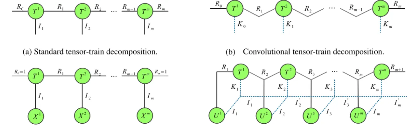
In this section, we introduce the basic concepts oftensor diagramsandtensor operations. These concepts will serve as building blocks for higher-order models (in particular, tensor-train models) in the next section.

Tensor Diagrams. Following the convention in quantum physics (Cichocki et al.,2016), we introduce tensor di-agrams in Figure 1, graphical representations of multi-dimensional arrays. In these diagrams, an array is repre-sented as avertex (node), whoseorderis denoted by the number ofedges (links)connected to the node, where each edge corresponding to amode (axis). Thedimensionof a mode is denoted by a number with the corresponding edge.

c (a) Scalar v I (b) Vector M I J (c) Matrix T I J K (d) Tensor Figure 1.Tensor diagrams of a scalarc∈R, a vectorv∈RI, a matrixM∈RI×Jand a third-order tensorT ∈RI×J×K. Tensor Operations.With these diagrams, we can represent the operations between (higher-order) tensors graphically. In Figure2, we illustrate threetensor operationscommonly used in neural networks, namelytensor contraction,tensor convolutionandbatch product. In these figures, an oper-ation is denoted by connecting the edges from both input tensors, where the type of operation is distinguished by the shape/color of the edges: solid line stands for tensor con-traction or batch product, and dotted line represents tensor convolution. Notice that a tensor operation can be arbitrarily complicated by linking multiple edges from multiple tensors simultaneously, see Figure4for an example.

4. Tensor-Trains and Sequence Modeling

The goal of tensor decomposition is to represent a higher-order tensor in a set of smaller and lower-higher-ordercore tensors, with fewer parameters while preserving essential informa-tion.Yu et al.(2017) usedtensor-train decomposition( Os-eledets,2011) to reduce both parameters and computations in higher-order recurrent model. We will review the standard model in the first part of this section.

However, the approach byYu et al.(2017) only considers recurrent models with vector inputs. Since spatial struc-ture is not preserved by standard tensor-train decomposition, their approach cannot be tensor-train cannot be extended to cope with video/image inputs directly. In the second part, we propose a novelConvolutional Tensor-Train

De-composition(CTTD). With CTTD, a large convolutional kernel is factorized into a chain of smaller kernels. We show that such decomposition can significantly reduce both parameters and operations of higher-order spatio-temporal recurrent models.

Throughout this section, We will use tensor diagrams to illustrate the operations in all models. The exact mathemati-cal expression for these models are included in Appendix A.

Standard Tensor-Train Decomposition. Given anm -ordertensorT ∈RI1×···×Im _with_I

las thedimensionof

itsl-thmode, a standard tensor-train decomposition (TTD) factorizes the tensorT into a set ofmcore tensors{Tl_}m

l=1

withTl_∈

RIl×Rl×Rl+1_{, illustrated in Figure}_3a_{. In TTD,} theranks{Rl}ml=1−1control the number of parameters in thetensor-train format, and the original tensorT of size (Qm

l=1Il)is compressed to(

Pm

l=1IlRl−1Rl), i.e. the com-plexity of TTD only grows linearly with the orderm (assum-ingRl’s are constants). Therefore, TTD is commonly used

to approximate higher-order tensors with fewer parameters. As shown in Figure3a, the tensor diagram for TTD takes a “train” shape (and therefore its name). The sequential structure in TTD makes it particularly suitable for sequence modeling. Consider a higher-order model that predicts a scalar outputy∈Rbased on the outer product of a sequence

of input vectors{xl_}m l=1withx l_∈ RIl_, y= T, x1⊗x2· · · ⊗xm (1) This model is intractable in practice since the number of parameters inT ∈RI1×···Im_{(and therefore computational}

complexity) grows exponentially with the orderm. Now supposeT takes a tensor-train format as in Figure3a, Equa-tion (1) can be efficiently evaluated sequentially from left to right as in Figure3c:x1_{first interacts with}_T1_{, and the} intermediate result interacts withT2_and_x2_{simultaneously,} and so on. Notice that the higher-order tensorT is never reconstructed in the process, therefore both space and com-putational complexities grow linearly (not exponentially as in Equation (1)) with the orderm.

Convolutional Tensor-Train Decomposition. A convo-lutional layer (in neural networks) is typically parameter-ized by a tensorT ∈ RK×R1×Rm+1_{, where}_K_{is the} ker-nel size, andR1,Rm+1 are the number of input and out-put channels. Suppose the kernel size K takes the form

K= (Pm

l=1Kl)−m+ 1, we propose convolutional

tensor-train decomposition (CTTD) that factorizesT into a set ofmcore tensors{Tl_}m

l=1withT

l_∈

RKl×Rl×Rl−1 _{as in} Figure3b, and denoteT =CTTD({Tl_}m

l=1). As in TTD, theranksof CTTD{Rl}ml=1control the complexity of the convolutional tensor-train format, and the number of param-eters reduces fromKR1Rm+1toP

m

l=1KlRlRl+1.

(4)

T1 I _T2 M J K N J K N M = T

(a) Tensor contraction.

Tj,k,m,n=P_iTi,j,k1 T 2 i,m,n T1 I T2 M J K N J K N M T ₌ I L I ' (b) Tensor convolution. T:,j,k,m,n=T:1,j,k∗ T 2 :,m,n T1 _I _T2 M J K N J K N M = T I (c) Batch product. Ti,j,k=Ti,j,k2 T 2 i,m,n

Figure 2.Diagrams of tensor operations. For all examples, the inputs are two third-order tensorsT1_∈

RI×J×KandT2∈RI×M×N, and the operations are on modeI. (a)In tensor contraction, the edges for operation must share the same dimension, and will vanish after contraction;(b)In tensor convolution, a new edge will emerge after the operation. Different from contraction, the dimensions for the operating edges may be different depending on the type of convolution.(c)In batch product, a new edge will also emerge after the operation. Different from convolution, the dimensions for all operating edges must be the same.

T1 R1 _T2 R2 ... Rm−1 _Tm

R0 Rm

I1 I2 Im

(a) Standard tensor-train decomposition.

T1 _T2 ... _Tm

R0 Rm

K0 K1 Km

R1 R2 Rm−1

(b) Convolutional tensor-train decomposition.

T1 R1

T2 R2 ... Rm−1 _Tm

R0=1 Rm=1

I1 I2 Im

X1 _X2 _Xm

(c) Standard tensor-train for sequence modeling.

T1 T2 ... Tm R1 Rm+1 K1 K2 Km R2 R3 Rm U1 U2 U3 _Um I1 I2 K3 I3 Im I1 ' I2 ' I3 ' Im '

(d) Convolutional tensor-train for spatial-temporal modeling. Figure 3.(1)In the first row, we illustrate the tensor diagrams for both standard tensor-train decomposition and convolutional tensor-train decomposition. Notice that convolutional TTD is different from the standard TTD in that it replaces dangling edges{Il}ml=1for contraction by ones{Kl}ml=1for convolution.(2)In the second row, we illustrate the applications of both tensor-train decompositions in sequence modeling. (c) In standard TTD, all edges{I1}ml=1and{Rl}m−1l=1 are contracted. (d) In convolutional TTD, the edges{Il}ml=1are contracted, and edges{Il}ml=1and{Kl}ml=1are involved in convolutions. Notice that in convolutional TTD, the edges{Rl}ml=1for contraction is not directly linked to any vertex in order to avoid an extra dimension inTl_{. Both models can be evaluated by interacting the} tensors from left to right to obtain the final output and takeFigure 3dfor an example:U1

is first interacted withT1

, and the resulted tensor is further interacted withT2_and_U2_{. The process repeats until all tensors are merged into one.}

be used to compress higher-order spatio-temporal recurrent models with convolutional operations. Consider a model that predicts a featureV ∈RI

0 m×Rm+1_{based on a sequence} of input features{Ul_}m l=1withU l _∈ RIl×Rl_(where_I lis

the feature length, andRlis the number of channels inUl),

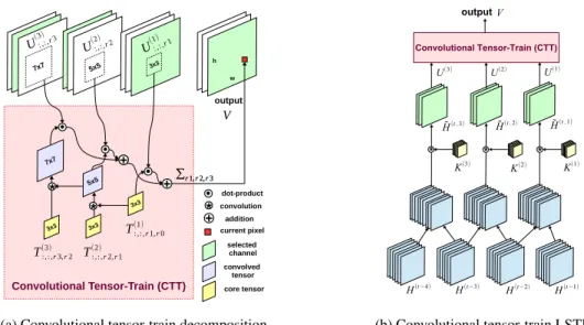
V:,:,rm+1 = m X l=1 Wl :,:,rl,rm+1∗ U l :,:,rl withWl₌ CTTD {Tk_}m k=l (2)

whereWl_{is the corresponding weights tensor for}_Ul_{, which}

itself takes takes a convolutional tensor-train format in Fig-ure3b. The structure also admits an efficient algorithm:U1 is first interacted withT1_{, and the result is further interacted} withT2_and_U2_{simultaneously. The process is illustrated} in Figure3d. Again, the original weightsWl_{’s are never}

reconstructed in such a process. The overall operations of a third-order CTTD (Equation (2)) for two-dimensional fea-tures are illustrated in Figure4a. In this paper, we denote Equation (2) simply asV=CTT({Tl_}m

l=1,{U

l_}m

l=1).

5. Convolutional Tensor-Train LSTM

Convolutional LSTM (ConvLSTM) is a basic building block for most recent video forecasting models (Xingjian et al.,

2015), where the spatial information is encoded explicitly as tensors in the LSTM cells. In a ConvLSTM network, each cell is a first-order Markov model, where the hidden state is updated based on its previous step. In this section, we pro-pose Convolutional Tensor-Train LSTM (Conv-TT-LSTM), where ConvLSTM is integrated with convolutional tensor-train to model higher-order spatio-temporal correlations explicitly. The proposed model is illustrated inFigure 4. Notations.In this section,∗is overloaded to denote convolu-tion between higher-order tensors. For instance, given a4-th order weights tensorW ∈RK×K×S×Cand a3-rd order

in-put tensorX ∈RH×W×S,Y=W ∗Xcomputes a3-rd

out-put tensorY ∈RH×W×TasY:,:,c=Ps=1W:,:,s,c∗ X:,:,s.

The symbol◦is used to denote element-wise product be-tween two tensors, andσrepresents a function that performs

(5)

3x3 3x3 7x7 3x3 5x5 * + + * + w h Convolutional Tensor-Train (CTT) V dot-product convolution addition current pixel selected channel ∑r1,r2,r3 ∑r1,r2,r3 output 7x7 _5x5 3x3 convolved tensor core tensor U(3:,):,r3 U(2:,:,r) 2 U(1:,):,r1 T:,:,r3,r2 (3) _T :,:,r2,r1 (2) T:,:,r1,r0 (1) * * + + +*

(a) Convolutional tensor-train decomposition.

Convolutional Tensor-Train (CTT) output H(t−4) _H(t−3) _H(t−2) K(3) _K(2) _K(1) V * * * ̃ H(t ,3) _H_̃(t ,2) _H_̃(t ,1) H(t−1) (b) Convolutional tensor-train LSTM

Figure 4.Illustration of (a) convolutional tensor-train decomposition(Equation (2)) and (b) convolutional tensor-train LSTM (Equation (6)). The original frames to Conv-TT-LSTM are first grouped by a sliding window before fed into the convolutional tensor-train. In Conv-TT-LSTM, the CTTD is used with two minor modifications: (1) The edges for convolutions are extended to two-dimensional, i.e.

IlandKlin Figure3dare tuples of two dimensionsIl= (H, W)andKl= (k, k); (2) The indices are named reversely such that they reflect the number of steps from the current output, e.g.U(3)₌_U1_and_U(1)₌_U3_{in Figure}_3d_.

element-wise (nonlinear) transformation on a tensor. Convolutional Long Short-Term Memory (ConvLSTM).

Xingjian et al.(2015) extended fully-connected LSTM to Convolutional LSTM to model spatio-temporal structures within each recurrent unit, where all features are encoded as third-order tensors with dimensions (heightH×width

W ×channelsC) and operations are replaced by convo-lutions between tensors. In each cell, the parameters are characterized by two4-th order tensorsW ∈RK×K×S×4C

andT ∈RK×K×C×4C, whereKis the kernel size for

con-volutions,S,Care the numbers of channels of the inputs X(t)_∈

RH×W×Sand hidden statesH(t)∈RH×W×C. At

each time stept, a cell updates its hidden statesH(t)_based on the previous stepH(t−1)_{and the current input}_X(t)_.

[I(t)_;_F(t)_;_C_˜(t)_;_O(t)_{] =}_σ₍_{W ∗ X}(t)₊_{T ∗ H}(t−1)₎ ₍₃₎ C(t)₌_C_˜(t)_{◦ I}(t)_; _H(t)₌_O(t)_{◦ C}(t) ₍₄₎ whereσ(·)applies sigmoid on the input gateI(t)_{, forget} gateF(t)_{, output gate}_O(t)_{, and}_tanh(_·₎_{on memory cell}

˜

C(t)_{. Notice that}_C(t)_,_I(t)_,_F(t)_,_O(t)_∈

RH×W×Care all

3-rd order tensors.

Convolutional Tensor-Train LSTM (Conv-TT-LSTM). We introduce a higher-order recurrent unit to capture multi-steps spatio-temporal correlations in ConvLSTM, where the hidden state H(t)_{is updated based on its} _n_previous steps{H(t−l)_}n

l=1with anm-orderCTTas in Equation2. Concretely, suppose the parameters inCTTare character-ized bymtensors of4-th order{T(o)_}m

o=1, Conv-TT-LSTM

replaces Equation (3) in ConvLSTM by two equations:

˜ H(t,o)₌_f_K(o)_, _{H(t−l)_}n l=1 ,∀o∈[m] (5) I(t)_;_F(t)_;_C_˜(t)_;_O(t) =σ W ∗ X(t)₊ CTT {T(o)_}m o=1,{H˜ (t,o)_}m o=1 (6) (1)SinceCCT({T(l)_}m

l=1,·)takes a series ofmtensors as inputs, the first step in (5) maps theninputs{H(t−l)_}n

l=1

to m intermediate tensors {H(t,o)_}m

o=1 with a function

f. (2) These m tensors {H˜(t,o)_}m

o=1 are then fed into CCT({T(l)_}m

l=1,·)and compute the gates per Equation (6). In this work, we devise asliding windowstrategy to com-pute Equation (5). With this strategy, a sliding subset of {H(l)_} _{are concatenated into}_H_ˆ(t,o)_{, which is then} trans-formed into an inputH˜(t,o)_{to the convolutional tensor-train} (See Figure4b). Concretely, the Conv-TT-LSTM model computes eachH˜(t,o)_{by the following equation:}

˜

H(t,o)₌_K(o)_∗_H_ˆ(t,o) =K(o)_∗

H(t−n+m−l)_;_{· · · H}(t−l) (7)

Thenprevious states{H(l)_}n

l=1are first concatenated (over time axis) intomtensors{Hˆ(t,o)_}m

o=1by a sliding window, each of which has sizeHˆ(t,o)_∈

RH×W×D×C (withD =

n−m+ 1) and thereafter mapped toH˜(t,o)_∈

RH×W×R

by 3D-convolution with a kernelK(l)_∈

Rk×k×D×R.

We note that afixing windowstrategy is also feasible here, where allUl’s are concatenated into a single tensor, which repeatedly used in every single input. The discussion of

(6)

fixed window and the empirical comparison against sliding window are shown in Appendix B.

6. Experiments

We first evaluate our approach on the synthetic Moving-MNIST-2 dataset (Srivastava et al.,2015). In addition, we use KTH human action dataset (Laptev et al.,2004) to test the performance of our proposed models in more realistic scenario.

Model Architecture. All experiments use a stack of 12-layers of ConvLSTM or Conv-TT-LSTM with 32 channels for the first and last 3 layers, and 48 channels for the 6 layers in the middle. A convolutional layer is applied on top of all recurrent layers to compute the predicted frames, fol-lowed by an extra sigmoid layer for colored videos. Follow-ingByeon et al.(2018), two skip connections performing concatenation over channels are added between (3, 9) and (6, 12) layers. Illustration of the network architecture is included in Appendix D.All parameters are initialized by Xavier’s normalized initializer (Glorot & Bengio,2010) and initial states in ConvLSTM or Conv-TT-LSTM are initial-ized as zeros.

Evaluation Metrics. We use two traditional metrics MSE (or PSNR) and SSIM (Wang et al.,2004), and a recently proposed deep-learning based metric LPIPS (Zhang et al.,

2018), which measures the similarity between deep features. Since MSE (or PSNR) is based on pixel-wise difference, it favors vague and blurry predictions, which is not a proper measurement of perceptual similarity. While SSIM was originally proposed to address the problem,Zhang et al.

(2018) shows that their proposed LPIPS metric aligns better to human perception.

Learning Strategy. All models are trained with ADAM optimizer (Kingma & Ba,2014) withL1+L2loss. Learning rate decay and scheduled sampling (Bengio et al.,2015) are used to ease training. Scheduled sampling is started once the model does not improve in20epochs (in term of validation loss), and the sampling ratio is decreased linearly from1 until it reaches zero (by2×10−4each epoch for Moving-MNIST-2 and5×10−4for KTH). Learning rate decay is further activated if the loss does not drop in 20 epochs, and the rate is decreased exponentially by0.98every5epochs. Hyper-parameters Selection. We perform a wide range of hyper-parameters search for Conv-TT-LSTM to identify the best model. The full list of search values are summarized in Table4(Appendix C).The initial learning rate of10−3_is found for baseline ConvLSTM and10−4_{for our proposed} Conv-TT-LSTM. We found that the Conv-TT-LSTM models suffer from exploding gradients when learning rate is high, therefore we also explore various gradient clipping values and select1for all models. All other hyper-parameters are

selected using the best validation performance. 6.1. Moving-MNIST-2 Dataset

The Moving-MNIST-2 dataset is generated by moving two digits of size28×28in MNIST dataset within a64×64 black canvas. These digits are placed at a random initial location, and move with constant velocity in the canvas and bounce when they reach the boundary. FollowingWang et al.(2018a), we generate 10,000 videos for training, 3,000 for validation, and 5,000 for test with default parameters in the generator5. All our models are trained to predict 10 frames given 10 input frames.

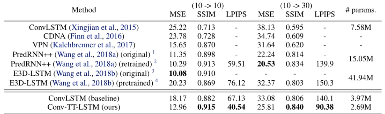
Multi-Steps Prediction. Table1reports the average statis-tics for 10 and 30 frames prediction, and Figure5shows comparison of per-frame statistics for PredRNN++ model, ConvLSTM baseline and our proposed Conv-TT-LSTM model.(1)Our Conv-TT-LSTM model consistently outper-form the 12-layer ConvLSTM baseline for both 10 and 30 frames predictionwith fewer parameters;(2)The Conv-TT-LSTM outperform previous approaches in terms of SSIM and LPIPS (especially on 30 frames prediction),with less than one fifth of the model parameters.

We reproduce the PredRNN++ model (Wang et al.,2018a) from their source code2, and we find that (1) The Pre-dRNN++ model tends to output vague and blurry results in long-term prediction (especially after 20 steps).(2)and our Conv-TT-LSTMs are able to produce sharp and realistic digits over all steps. An example of comparison for different models is shown in Figure6. The visualization is consistent with the results in Table1and Figure5.

Ablation Studies on CTTD The core component in our Conv-TT-LSTM is a higher-order convolutional TTD. In the following ablation studies, we present the necessity of (1) higher-order model and (2) convolutional operations in the decomposition for capturing long-term spatio-temporal information. We compare the performance of two ablated models against our Conv-TT-LSTM in Table3. The single

1

The results are cited from the original paper (Wang et al.,

2018a), where the miscalculation of MSE is corrected in the table. 2_{The results for PredRNN++ are reproduced from} _https:

//github.com/Yunbo426/predrnn-pp with the same datasets in this paper. The original implementation crops each frame into patches as the input to the model. We find such pre-processing is unnecessary and the performance of reproduced model is better than the one in the original paper.

3_{The results for E3D-LSTM are cited from the original} pa-per (Wang et al.,2018b).

4_{The results are reproduced with the pretrained model by the} authorshttps://github.com/google/e3d_lstm.

5

The Python code for Moving-MNIST-2 generator is publicly available online in https://github.com/jthsieh/ DDPAE-video-prediction/blob/master/data/ moving_mnist.py.

(7)

Table 1.Comparison of 10 and 30 frames prediction on Moving-MNIST-2 test set, where lower MSE values (in10−3) / higher SSIM / lower LPIPS values (in10−3) indicate better results. The reported Conv-TT-LSTM model is with order 3, steps 3, and ranks 8.

Method (10 -> 10) (10 -> 30) # params.

MSE SSIM LPIPS MSE SSIM LPIPS

ConvLSTM (Xingjian et al.,2015) 25.22 0.713 - 38.13 0.595 - 7.58M

CDNA (Finn et al.,2016) 23.78 0.728 - 34.74 0.609 -

-VPN (Kalchbrenner et al.,2017) 15.65 0.870 - 31.64 0.620 - -PredRNN++ (Wang et al.,2018a) (original)1 11.35 0.898 - 22.24 0.814

-15.05M PredRNN++ (Wang et al.,2018a) (retrained)2 _10.29 _0.913 _59.51 _20.53 _0.834 _139.9

E3D-LSTM (Wang et al.,2018b) (original)3 10.08 0.910 - - -

-41.94M E3D-LSTM (Wang et al.,2018b) (pretrained)4 20.23 0.869 76.12 32.37 0.803 150.3

ConvLSTM (baseline) 18.17 0.882 67.13 33.08 0.806 140.1 3.97M

Conv-TT-LSTM (ours) 12.96 0.915 40.54 25.81 0.840 90.38 2.69M

Table 2.Evaluation of multi-steps prediction on KTH dataset, where higher PSNR/SSIM values and lower LPIPS values indicate better predictive results. The reported Conv-TT-LSTM model here is with order 3, steps 3, and ranks 8. Our Conv-TT-LSTM outperforms ConvLSTM baseline and all previous approach in terms of SSIM and LPIPS.

Method (10 -> 20) (10 -> 40) # Parameters

PSNR SSIM LPIPS PSNR SSIM LPIPS

ConvLSTM (Xingjian et al.,2015) 23.58 0.712 - 22.85 0.639 - 7.58M

MCNET (Villegas et al.,2017) 25.95 0.804 - - - -

-PredRNN++ (Wang et al.,2018a) (original)1 _28.46 _0.865 _- _25.21 _0.741

-15.05M PredRNN++ (Wang et al.,2018a) (retrained)2 28.62 0.888 228.9 26.94 0.865 279.0

E3D-LSTM (Wang et al.,2018b) (original)3 29.31 0.879 - 27.24 0.810

-41.94M E3D-LSTM (Wang et al.,2018b) (pretrained)4 27.92 0.893 298.4 26.55 0.878 328.8

ConvLSTM (baseline) 28.21 0.903 137.1 26.01 0.876 201.3 3.97M

Conv-TT-LSTM (ours) 28.36 0.907 133.4 26.11 0.882 191.2 2.69M

Table 3.Ablation studies of higher-order Conv-TT-LSTM model. In these experiments, we evaluate the necessity of (1) higher-order model and (2) convolutional operations in the decomposition. The experimental results show that the ablated Conv-TT-LSTMs have similar performance to the ConvLSTM baseline.

Conv-TT-LSTM (10 -> 30) # parameters MSE(×10−3) SSIM LPIPS

CTTD with1×1filters (similar to standard TTD) single order 31.52 0.810 148.7 2.36M

order 3 34.84 0.800 151.2 2.37M

CTTD with5×5filters

single order 33.08 0.806 140.1 3.97M

order 3 28.88 0.831 104.1 2.65M

order means that the higher-order model is replaced to a first-order model (Tensor first-order=1). By replacing3×3filters to 1×1in CTTD, the effect of convolutions in CTTD is demon-strated compared to the standard TTD. The results show that the ablated models at best achieve similar performance of ConvLSTM baseline, which shows both higher-order model and convolutional operations are necessary for long-term video prediction.

6.2. KTH Action Dataset

KTH action dataset (Laptev et al.,2004) contains videos of 25 individuals performing 6 types of actions on a simple background. Our experimental setup followsWang et al.

(2018a), which uses persons 1-16 for training and 17-25 for testing, and each frame is resized to128×128pixels. All our models are trained to predict 10 frames given 10 input frames. During training, we randomly select 20 contiguous frames from the training videos as a sample and group every 10,000 samples into one epoch to apply the learning strategy as explained at the beginning of this section.

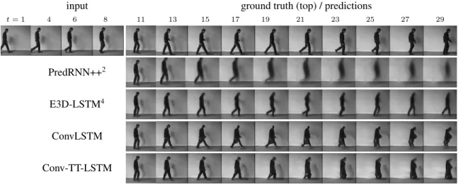
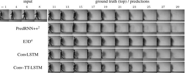
Results. In Table2, we report the evaluation on both 20 and 40 frames prediction.(1)Our models are consistently better than the ConvLSTM baseline for both 20 and 40 frames prediction.(2)While our proposed Conv-TT-LSTMs achieve lower SSIM value compared to the state-of-the-art models in 20 frames prediction, they outperform all previous models in LPIPS for both 20 and 40 frames prediction. An example of the predictions by the baseline and Conv-TT-LSTMs is shown in Figure6.

(8)

Figure 5.Frame-wise comparison in MSE, SSIM and PIPS on Moving-MNIST-2 dataset. For MSE and LPIPS, lower curves denote higher quality; while for SSIM, higher curves imply better quality. Our Conv-TT-LSTM performs better than ConvLSTM baseline, PredRNN++ (Wang et al.,2018a) and E3D-LSTM (Wang et al.,2018b) in all metrics (except for PredRNN++ in term of MSE).

input ground truth (top) / predictions

t= 1 4 6 8 11 14 17 20 23 26 29 32 35 38

PredRNN++2

E3D-LSTM4

ConvLSTM

Conv-TT-LSTM

Figure 6.30 frames prediction on Moving-MNIST given 10 input frames. Every 3 frames are shown. The first frames (t= 1and11) are animations. To view the animation, Adobe reader is required.

t= 1 4 6 8 11 13 15 17 19 21 23 25 27 29

PredRNN++2

E3D-LSTM4

ConvLSTM

Conv-TT-LSTM

Figure 7.20 frames prediction on KTH given 10 input frames. Every 2 frames are shown. The first frames (t= 1and11) are animations. To view the animation, Adobe reader is required.

(9)

7. Conclusion

In this paper, we proposedConvolutional Tensor-Train De-composition(CTTD) to factorize a large convolutional ker-nel into a set of smallercore tensors. We applied CTTD to efficiently constructconvolutional tensor-train LSTM (Conv-TT-LSTM), a higher-order recurrent neural network, that is capable to effectively capture long-term spatio-temporal correlations. We demonstrated the capacity of our proposed Conv-TT-LSTM on video prediction, and showed our model outperforms standard ConvLSTM and produce better results compared to other state-of-the-art models with fewer param-eters. Utilizing the proposed model for high-resolution videos is still challenging due to gradient vanishing or ex-plosion. Future direction will include investigating other training strategies or model designs to ease the training.

References

Alahi, A., Goel, K., Ramanathan, V., Robicquet, A., Fei-Fei, L., and Savarese, S. Social lstm: Human trajectory prediction in crowded spaces. InProceedings of the IEEE conference on computer vision and pattern recognition, pp. 961–971, 2016.

Anandkumar, A., Ge, R., Hsu, D., Kakade, S. M., and Tel-garsky, M. Tensor decompositions for learning latent variable models. The Journal of Machine Learning Re-search, 15(1):2773–2832, 2014.

Babaeizadeh, M., Finn, C., Erhan, D., Campbell, R. H., and Levine, S. Stochastic variational video prediction.arXiv preprint arXiv:1710.11252, 2017.

Bengio, S., Vinyals, O., Jaitly, N., and Shazeer, N. Sched-uled sampling for sequence prediction with recurrent neu-ral networks. InAdvances in Neural Information Process-ing Systems, pp. 1171–1179, 2015.

Byeon, W., Wang, Q., Kumar Srivastava, R., and Koumout-sakos, P. Contextvp: Fully context-aware video predic-tion. InProceedings of the European Conference on Computer Vision (ECCV), pp. 753–769, 2018.

Cichocki, A., Lee, N., Oseledets, I., Phan, A.-H., Zhao, Q., Mandic, D. P., et al. Tensor networks for dimensionality reduction and large-scale optimization: Part 1 low-rank tensor decompositions. Foundations and TrendsR in Machine Learning, 9(4-5):249–429, 2016.

Denton, E. and Fergus, R. Stochastic video generation with a learned prior. In35th International Conference on Machine Learning, ICML 2018, pp. 1906–1919. Interna-tional Machine Learning Society (IMLS), 2018.

Denton, E. L. et al. Unsupervised learning of disentan-gled representations from video. InAdvances in neural information processing systems, pp. 4414–4423, 2017. Finn, C. and Levine, S. Deep visual foresight for planning

robot motion. In2017 IEEE International Conference on Robotics and Automation (ICRA), pp. 2786–2793. IEEE, 2017.

Finn, C., Goodfellow, I., and Levine, S. Unsupervised learning for physical interaction through video prediction. InAdvances in neural information processing systems, pp. 64–72, 2016.

Glorot, X. and Bengio, Y. Understanding the difficulty of training deep feedforward neural networks. In Pro-ceedings of the thirteenth international conference on artificial intelligence and statistics, pp. 249–256, 2010. Hochreiter, S. and Schmidhuber, J. Long short-term memory.

(10)

Hsieh, J.-T., Liu, B., Huang, D.-A., Fei-Fei, L. F., and Niebles, J. C. Learning to decompose and disentangle representations for video prediction. InAdvances in Neu-ral Information Processing Systems, pp. 517–526, 2018. Kalchbrenner, N., van den Oord, A., Simonyan, K., Dani-helka, I., Vinyals, O., Graves, A., and Kavukcuoglu, K. Video pixel networks. InProceedings of the 34th Interna-tional Conference on Machine Learning-Volume 70, pp. 1771–1779. JMLR. org, 2017.

Kim, Y.-D., Park, E., Yoo, S., Choi, T., Yang, L., and Shin, D. Compression of deep convolutional neural networks for fast and low power mobile applications.arXiv preprint arXiv:1511.06530, 2015.

Kingma, D. P. and Ba, J. Adam: A method for stochastic optimization. arXiv preprint arXiv:1412.6980, 2014. Kolbeinsson, A., Kossaifi, J., Panagakis, Y., Anandkumar,

A., Tzoulaki, I., and Matthews, P. Stochastically rank-regularized tensor regression networks. arXiv preprint arXiv:1902.10758, 2019.

Kolda, T. G. and Bader, B. W. Tensor decompositions and applications.SIAM review, 51(3):455–500, 2009. Kossaifi, J., Lipton, Z., Khanna, A., Furlanello, T., and

Anandkumar, A. Tensor regression networks. arXiv, 2017.

Kossaifi, J., Bulat, A., Panagakis, Y., and Pantic, M. Effi-cient n-dimensional convolutions via higher-order factor-ization. arXiv preprint arXiv:1906.06196, 2019. Laptev, I., Caputo, B., et al. Recognizing human actions: a

local svm approach. Innull, pp. 32–36. IEEE, 2004. Lebedev, V., Ganin, Y., Rakhuba, M., Oseledets, I., and

Lempitsky, V. Speeding-up convolutional neural net-works using fine-tuned cp-decomposition.arXiv preprint arXiv:1412.6553, 2014.

Lee, A. X., Zhang, R., Ebert, F., Abbeel, P., Finn, C., and Levine, S. Stochastic adversarial video prediction.arXiv preprint arXiv:1804.01523, 2018.

Lotter, W., Kreiman, G., and Cox, D. Deep predictive coding networks for video prediction and unsupervised learning.arXiv preprint arXiv:1605.08104, 2016. Ma, X., Zhang, P., Zhang, S., Duan, N., Hou, Y., Song,

D., and Zhou, M. A tensorized transformer for language modeling. arXiv preprint arXiv:1906.09777, 2019. Mathieu, M., Couprie, C., and LeCun, Y. Deep

multi-scale video prediction beyond mean square error.arXiv preprint arXiv:1511.05440, 2015.

Novikov, A., Podoprikhin, D., Osokin, A., and Vetrov, D. P. Tensorizing neural networks. InAdvances in neural in-formation processing systems, pp. 442–450, 2015.

Oseledets, I. V. Tensor-train decomposition. SIAM Journal on Scientific Computing, 33(5):2295–2317, 2011. Soltani, R. and Jiang, H. Higher order recurrent neural

networks. arXiv preprint arXiv:1605.00064, 2016. Srivastava, N., Mansimov, E., and Salakhudinov, R.

Unsu-pervised learning of video representations using lstms. In International conference on machine learning, pp. 843– 852, 2015.

Su, J., Li, J., Bhattacharjee, B., and Huang, F. Tensorized spectrum preserving compression for neural networks. arXiv preprint arXiv:1805.10352, 2018.

Sutskever, I., Martens, J., and Hinton, G. E. Generating text with recurrent neural networks. InProceedings of the 28th International Conference on Machine Learning (ICML-11), pp. 1017–1024, 2011.

Tjandra, A., Sakti, S., and Nakamura, S. Compressing recurrent neural network with tensor train. In2017 Inter-national Joint Conference on Neural Networks (IJCNN), pp. 4451–4458. IEEE, 2017.

Vaswani, A., Shazeer, N., Parmar, N., Uszkoreit, J., Jones, L., Gomez, A. N., Kaiser, Ł., and Polosukhin, I. Atten-tion is all you need. InAdvances in neural information processing systems, pp. 5998–6008, 2017.

Villegas, R., Yang, J., Hong, S., Lin, X., and Lee, H. De-composing motion and content for natural video sequence prediction. arXiv preprint arXiv:1706.08033, 2017.

Wang, Y., Long, M., Wang, J., Gao, Z., and Philip, S. Y. Predrnn: Recurrent neural networks for predictive learn-ing uslearn-ing spatiotemporal lstms. InAdvances in Neural Information Processing Systems, pp. 879–888, 2017. Wang, Y., Gao, Z., Long, M., Wang, J., and Yu, P. S.

Predrnn++: Towards a resolution of the deep-in-time dilemma in spatiotemporal predictive learning. arXiv preprint arXiv:1804.06300, 2018a.

Wang, Y., Jiang, L., Yang, M.-H., Li, L.-J., Long, M., and Fei-Fei, L. Eidetic 3d lstm: A model for video prediction and beyond.preprint, 2018b.

Wang, Z., Bovik, A. C., Sheikh, H. R., Simoncelli, E. P., et al. Image quality assessment: from error visibility to structural similarity.IEEE transactions on image process-ing, 13(4):600–612, 2004.

(11)

Weissenborn, D., Täckström, O., and Uszkoreit, J. Scal-ing autoregressive video models. arXiv preprint arXiv:1906.02634, 2019.

Xingjian, S., Chen, Z., Wang, H., Yeung, D.-Y., Wong, W.-K., and Woo, W.-c. Convolutional lstm network: A machine learning approach for precipitation nowcasting. InAdvances in neural information processing systems, pp. 802–810, 2015.

Yang, Y., Krompass, D., and Tresp, V. Tensor-train recur-rent neural networks for video classification. In Proceed-ings of the 34th International Conference on Machine Learning-Volume 70, pp. 3891–3900. JMLR. org, 2017. Yu, R., Zheng, S., Anandkumar, A., and Yue, Y.

Long-term forecasting using tensor-train rnns.arXiv preprint arXiv:1711.00073, 2017.

Zhang, R., Isola, P., Efros, A. A., Shechtman, E., and Wang, O. The unreasonable effectiveness of deep features as a perceptual metric. InProceedings of the IEEE Conference on Computer Vision and Pattern Recognition, pp. 586– 595, 2018.

Zhang, S., Wu, Y., Che, T., Lin, Z., Memisevic, R., Salakhut-dinov, R. R., and Bengio, Y. Architectural complexity measures of recurrent neural networks. InAdvances in neural information processing systems, pp. 1822–1830, 2016.

(12)

Appendix: Convolutional Tensor-Train LSTM for Spatio-temporal Learning

A. Mathematical Expressions for Tensor-Trains

In Section4, we introduced the concepts of standard and convolutional tensor-trains and their applications in sequence modeling intensor diagrams. In this section, we present their equivalent forms inmathematical expressions.

A.1. Standard Tensor-Train Decomposition and Temporal Modeling

Notice that tensor diagram of standard tensor-train inFigure 3acan be expressed as Ti1,···,im , R1 X r1=1 · · · Rm−1 X rm−1=1 T1 i1,1,r1 · · · T m im,rm−1,1 (8)

and the higher-order regressive model inEquation 1can be rewritten as

y= I1 X i1=1 · · · Im X im=1 Ti1,···,imx 1 i1 · · · x m im (9)

Then the sequential algorithm illustrated inFigure 3cis equivalent to v_rl l= Il X il=1 Rl X rl−1=1 Till,rl−1,rlv l−1 rl−1 x l il (10)

where the vectors{vl_}m

l=1(withv

l_∈

RRl_{) are intermediate steps, with initial input}_v0_{= 1}_{, and final output}_y₌_vm_{. We}

will prove the correctness of this algorithm by induction.

Proof ofEquation 10 We denote the standard tensor-train decomposition inEquation 8asT =TTD({Tl_}m l=1), then

Equation 9can be rewritten asEquation 11sinceR0= 1andv (0) 1 = 1. v= R0 X r0=1 I1 X i1=1 · · · Im X im=1 TTD {Tl_}m l=1 i1,···,imv 0 r0 x 1_{⊗ · · · ⊗}_xm i1,···,im (11) = R0 X r0=1 I1 X i1=1 · · · Im X im=1   R1 X r1=1 · · · Rm−1 X rm−1=1 T1 i1,r0,r1· · · T m im,rm−1,rm  v 0 r0x 1 i1· · ·x m im (12) = R1 X r1=1 I2 X i2=1 · · · Im X im=1   R2 X r2=1 · · · Rm−1 X rm−1=1 T2 i2,r1,r2· · · T m im,rm−1,rm   R0 X r0=1 I1 X i1=1 T1 i1,r0,r1 v 0 r0x 1 i1 ! u2_i₂· · ·xm_i_m (13) = R1 X r1=1 I2 X i2=1 · · · Im X im=1 TTD {Tl}ml=2 i1,···,imv 1 r1 x 2 ⊗ · · · ⊗xm i2,···,im (14)

whereR0= 1,v01 = 1and the sequential algorithm inEquation 10is performed atEquation 13. A.2. Convolutional Tensor-Train Decomposition and Spatio-Temporal Modeling

Notice that the convolutional tensor-train inFigure 3bcan be expressed as T:,r1,rm+1 , R2 X r2=1 · · · Rm X rm=1 T1 :,r1,r2∗ · · · ∗ T m :,rm,rm+1 (15)

And the sequential algorithm illustrated inFigure 3dcan be equivalently stated as Vl+1 :,rl+1 = Rl X rl=1 Tl :,rl,rl+1∗ V l :,rl+U l :,rl (16)

(13)

where{Vl_}m

l=1(withV

l_∈

RH×W×Rl_{) are intermediate results, and}V1∈

RH×W×Rmis initialized as all zeros and final

prediction is returned asV=Vm+1_.

Proof ofEquation 16 We denote the convolutional tensor-train decomposition inEquation 15asT =CTTD(Tl₎m l=1, thenEquation 16can be rewritten asEquation 17sinceV1_{is an all zeros tensor.}

V:,rm+1 = m X l=1 Rl X rl=1 CTTD {Tt_}m t=l :,rl,rm+1∗ U l :,rl+ R1 X r1=1 CTTD {Tt_}m t=1 :,r1,rm+1∗ V 1 :,r1 (17) = m X l=2 Rl X rl=1 CTTD {Tt_}m t=l :,rl,rm+1∗ U l :,rl+ R1 X r1=1 CTTD {Tt_}m t=1 :,r1,rm+1∗ U 1 :,r1+V 1 :,r1 (18)

Note that the second term inEquation 18can now be simplified as

R1 X r1=1 CTTD {Tt_}m t=1 :,r1,rm+1∗ U 1 :,r1+V 1 :,r1 (19) = R1 X r1=1 R2 X r2=1 · · · Rm X rm=1 T1 :,r1,r2∗ · · · ∗ T m :,rm,rm+1 ! ∗ U1 :,r1+V 1 :,r1 (20) = R2 X r2=1 R3 X r3=1 · · · Rm X rm=1 T2 :,r2,r3∗ · · · ∗ T m :,rm,rm+1 ! ∗ "Rm X rm=1 T1 :,r1,r2∗ U 1 :,r1+V 1 :,r1 # (21) = R2 X r2=1 CTTD {Tt_}m−1 t=2 :,r2,rm+1∗ V 2 :,r2 (22)

where the sequential algorithm inEquation 16is performed to achieveEquation 22fromEquation 21. PluggingEquation 22

intoEquation 18, we reduceEquation 18back to the form asEquation 17. V:,rm+1= m X l=2 Rl X rl=1 CTTD {Tt_}m t=l :,rl,rm+1∗ U l :,rl+ R2 X r2=1 CTTD {Tt_}m−1 t=2 :,r2,rm+1∗ V 2 :,r2 (23) which completes the induction.

B. Model Details, Ablation Studies and Additional Experimental Results

B.1. Model Details

Details of the Architecture. All experiments use a stack of 12-layers of ConvLSTM or Conv-TT-LSTM with 32 channels for the first and last 3 layers, and 48 channels for the 6 layers in the middle. A convolutional layer is applied on top of all LSTM layers to compute the predicted frames, followed by an optional sigmoid function (In the experiments, we add sigmoid for KTH dataset but not for Moving-MNIST-2). Additionally, two skip connections performing concatenation over channels are added between (3, 9) and (6, 12) layers as is shown in Figure8.

Hyper-parameters Selection Table 4summarizes our search values

Kernel size Initial learning rate Tensor order Tensor rank Time steps {3, 5} {1e-4,5e-3,1e-3} {1,2,3,5} {4,8,16} {1,3,5}

Table 4.Hyper-parameters search values for Conv-TT-LSTM experiments.

B.2. Ablation Studies

Fixed Window Strategy. We investigate the another realization of Conv-TT-LSTM, i.e. a different implementation of Equation (5). With fixed window strategy, all previous steps{Hl_}n

(14)

Conv-(TT) LSTM X 3 Conv-(TT) LSTM X 3 Conv-(TT) LSTM X 3 Conv-(TT) LSTM X 3

Block 1 Block 2 Block 3 Block 4 Conv

48 units 48 units

32 units 32 units

σ

Input Output

Figure 8.Illustration of the network architecture for the 12-layers model used in the experiments.

ˆ

Ht _∈

RH×W×nC, which is repeatedly mapped tomtensors{H˜t,o ∈RH×W×R}mo=1by 2D-convolution with kernels {Ko_∈

Rk×k×nC×R}mo=1.

Conv-TT-LSTM (FW): H˜t,o=Ko∗Hˆt=Ko∗

Ht−n;· · ·;Ht−1

(24a) Conv-TT-LSTM (SW): H˜t,o₌_Ko_∗_H_ˆt,o₌_Ko_∗

Ht−n+m−l_;_{· · ·} _;_Ht−l

(24b) For comparison, we list the equations for both fixed window and sliding window strategies above. In Table5, we compare these two realizations on Moving-MNIST-2 under the same experimental setting, and we find that sliding window performs slightly better than fixed window.

Convolutional Tensor-Train (CTT) output H(t−3) _H(t−2) _H(t−1) K(3) K(2) K(1) V * * * ̃ H(t ,3) H̃(t ,2) H̃(t ,1) FW (a) Conv-TT-LSTM (FW) Convolutional Tensor-Train (CTT) output H(t−4) _H(t−3) _H(t−2) K(3) _K(2) _K(1) V * * * ̃ H(t ,3) _H_̃(t ,2) H̃(t ,1) H(t−1) SW (b) Conv-TT-LSTM (SW)

Figure 9.Illustration of two realizations of convolutional tensor-train LSTM.(a)InFixed Window (FW)realization, all steps are used to compute each input to convolutional tensor-train, while(b)inSliding Window (SW)realization, only steps in the window are used for computation at each input.

Ablation Study on our Experiment Setting. To understand whether our proposed Conv-TT-LSTM universally improves upon ConvLSTM (i.e. not tied to specific architecture, loss function and learning schedule), we perform three ablation studies on our experimental setting:(1)Reduce the number of layers from 12 layers to 4 layers (same as (Xingjian et al.,

2015) and (Wang et al.,2018a));(2)Change the loss function fromL1+L2toL1only;(3)Disable the scheduled sampling and use teacher forcing during training process. We evaluate the performance of ConvLSTM baseline and our proposed Conv-TT-LSTM under these ablated settings, and summarize their comparisons inTable 5. The results show that our proposed Conv-TT-LSTM consistently outperforms ConvLSTM for all settings, i.e. the Conv-TT-LSTM model improves upon ConvLSTM in a board range of setups, which is not limited to the certain setting used in our paper. These ablation studies further show that our setup is optimal for predictive learning in Moving-MNIST-2 dataset.

(15)

Model Layers Sched. Loss (10 -> 30) Params. 4 12 TF SS `1 `1+`2 MSE SSIM LPIPS

ConvLSTM -3 5 5 3 5 3 37.19 0.791 184.2 11.48M Conv-TT-LSTM FW 31.46 0.819 112.5 5.65M ConvLSTM -5 3 3 5 5 3 33.96 0.805 184.4 3.97M Conv-TT-LSTM FW 30.27 0.827 118.2 2.65M ConvLSTM -5 3 5 3 3 5 36.95 0.802 135.1 3.97M Conv-TT-LSTM FW 34.84 0.807 128.4 2.65M ConvLSTM -5 3 5 3 5 3 33.08 0.806 140.1 3.97M Conv-TT-LSTM FW 28.88 0.831 104.1 2.65M Conv-TT-LSTM SW 5 3 5 3 5 3 25.81 0.840 90.38 2.69M

Table 5.Evaluation of ConvLSTM and our Conv-TT-LSTMs under ablated settings. In this table, FW stands forfixed windowrealization, SW stands forsliding windowrealization; For learning scheduling, TF denotesteaching forcingand SS denotesscheduled sampling. The experiments show that(1)our Conv-TT-LSTM is able to improve upon ConvLSTM under all settings;(2)Our current learning strategy is optimal in the search space;(3)The sliding window strategy outperforms the fixed window one under the optimal experimental setting.

B.3. Additional Experimental Results

Per-frame metrics for KTH action dataset. The per-frame metrics are illustrated in Figure10.

Figure 10.Frame-wise comparison in PSNR, SSIM and PIPS on KTH action dataset. For LPIPS, lower curves denote higher quality; while for PSNR and SSIM, higher curves imply better quality. Our Conv-TT-LSTM performs better than ConvLSTM baseline, PredRNN++ (Wang et al.,2018a) and E3D-LSTM (Wang et al.,2018b) in terms of SSIM and LPIPS.

Additional Visual Results. We provide additional visual comparison among PredRNN++ (Wang et al.,2018a), E3D-LSTM (Wang et al.,2018b), our baseline ConvLSTM and our proposed Conv-TT-LSTM.

(16)

input ground truth (top) / predictions t= 1 4 6 8 11 14 17 20 23 26 29 32 35 38 PredRNN++2 E3D-LSTM4 ConvLSTM Conv-TT-LSTM

t= 1 4 6 8 11 14 17 20 23 26 29 32 35 38

PredRNN++2

E3D-LSTM4

ConvLSTM

Conv-TT-LSTM

t= 1 4 6 8 11 13 15 17 19 21 23 25 27 29

PredRNN++2

E3D4

ConvLSTM

Conv-TT-LSTM