Effective Prediction of Web User Behaviour
with User-Level Models
Krzysztof Dembczy ´nski, Wojciech Kotłowski
Institute of Computing Science, Pozna´n University of Technology 60-965 Pozna´n, Poland
Marcin Sydow∗
Web Mining Lab, Polish-Japanese Institute of Information Technology 02-008 Warszawa, Poland
Abstract. The paper concerns the problem of predicting behaviour of web users, based on real historical data which constitutes an important issue in web mining.
The research reported here was conducted while the authors participated in the international ECML/ PKDD 2007 Discovery Challenge competition – Track 1.
The results presented here ended up as the winning solution to the contest.
We describe the contest tasks and the real industrial datasets concerning the recorded behaviour of sample of Polish Web users on which our experiments were performed.
We present the whole extensive experimental process from the data preprocessing phase to ex-ploratory analysis of the data to the experimental comparison and discussion of various prediction models which we examined.
As we explain, our solution has low time and space complexity, scales well with large datasets and, at the same time, produces high-quality results.
Keywords: user behaviour prediction, web mining, machine learning, experimentation, data analy-sis
∗
Address for correspondence: Web Mining Lab, Polish-Japanese Institute of Information Technology, Koszykowa 86, 02-008 Warsaw, Poland
1.
Introduction
The paper concerns the problem of predicting behaviour of web users, based on real historical data which is of practical importance for many Internet-related companies and applications.
More specifically, it presents the research conducted by the authors which ended up as the winning solution to the international ECML/PKDD 2007 Discovery Challenge competition – Track 1. The task concerned prediction of the categories of web pages visited by web users, based on a large real training dataset provided by an industry company concerning over 500,000 recorded historical web sessions [1, 11]. The paper is an extension of [9], where our winning submission was initially described.
The goal of the paper is not only to present our solution to the competition task. We aimed at presen-ting the specific nature of the problem, which can be viewed at different levels of granularity. Choice of the granularity level has a crucial impact on the structure of the model. We analyse how the algorithms perform on various levels of granularity and come to conclusion that local models, treating each user separately, work best for the particular provided data. However, our analysis has potentially much wider relevance then only related to the dataset provided by the organisers of the contest: we believe the conclusions drawn in this paper may apply to the general problem of analysing web users’ behaviour.
1.1. Motivation and Related Work
The main motivation was to submit a high-quality solution to the competition. Our original submission is described in [9] while the solutions of other leading teams participating in the contest are reported in [17, 16].
However, apart from the fact, that our results described here were intended to be submitted as the contest solutions, the issue of web users’s behaviour prediction has very important practical applications. For example, predicting future behaviour of web users is a key issue inbehavioural targeting. Be-havioural targeting is a dynamically evolving area of web mining concerning optimising web on-line advertising, based on analysis of the web users’ behaviour. The user analysis approach is recently in the centre of interest in on-line advertising (e.g. [24]) and has a great potential in improving the perfor-mance of ad-serving systems which is proved by recent experiments [15]. As such, the issue constitutes a problem of high importance for industry and, at the same time is of high complexity.
There are more connections between our problem and on-line advertising. For instance, in dynam-ically growing market of search advertising [18], one often aims at determining the quality of the ad-vertisements to rank them on the search result page. The quality must be estimated from historical data [22, 23] either by investigating the popularity (measured with the number of clicks) of the particular advertisement in the past, or by extracting features from the content of the advertisement and using one of the machine learning methods. These two approaches share the characteristics of the models with the two approaches used in this paper (local and global models).
The problem of predicting a web page category a user might be interested in with use of keywords describing each category is reported in [19]. A model for demographic prediction based on user’s behav-iour is considered in [14].
1.2. Organisation of the paper
In Section 2 we describe the contest tasks, whose solutions were the main topic of our research presented in this paper. The section also describes the real training datasets provided by the contest organisers.
The exploratory data analysis phase, which was undertaken at the beginning of our research, is de-scribed in Section 3.
Since our solutions are mainly based on the statistical decision theory we briefly remind the basic concepts and denotations in Section 4.
Our solution to the Task 1 of the competition is presented in Section 5. We give a discussion of several different approaches which we examined.
We summarise and discuss all the experimental results for Task 1 obtained for all our approaches in Section 6.
The solutions to the remaining tasks (2 and 3) of the contest are presented in the Section 7. The final conclusions are contained in Section 8.
2.
Problem Description
The contest objective was to predict web users’ behaviour by characterising the nature of their visits. The visit is defined by categories of visited web pages and the number of page views in each category. The
Track 1of the contest was organised into three tasks:
1. predicting the number (‘1’ or ‘greater than 1’) of web page categories visited in a single session, 2. predicting the first 3 visited categories,
3. predicting the number of pages seen in each of the first 3 categories.
The data was provided by Gemius [2], a leading Internet market research company in Poland, and divided into two subsets, both representing some real recorded web sessions concerning 4882 web users, identified by cookies:
1. training set (379485 records), 2. testing set (166299 records).
The testing set contained almost exactly twice less records than the training one.
Each record contained the following attributes:record number,user id,timestamp
Additionally, in the training set each record consisted of the sequence of pairs, each of the following form: category,#pages
Each record corresponded to a user session started at timestamp and reflected the category and num-ber of pages seen by that user in chronological order (from left to right).
Example:
248 46 1167680792 12,1 8,7 12,3
which reads as ‘the user 46 during the session 248, which started at the time point 1167680792, has visited 1 page in category 12 then 7 pages in category 8 and finally 3 pages in category 12’
In addition, a third, auxiliary dataset was provided which contained 4882, user-related records con-sisting of the following attributes:
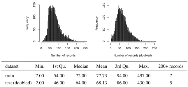
Train dataset Number of records Frequency 0 50 100 150 200 250 0 50 100 150 Test dataset
Number of records (doubled)
Frequency 0 50 100 150 200 250 0 50 100 150
dataset Min. 1st Qu. Median Mean 3rd Qu. Max. 200+ records train 7.00 54.00 72.00 77.73 94.00 497.00 7 test (doubled) 2.00 46.00 64.00 68.13 86.00 430.00 5
Figure 1. Summary of the statistics for the number of records per user in the training and testing (doubled) datasets. The typical number of records per user lies between 50 and 90 and does not vary very much but is not high enough (given the number of different categories, and other attributes) to build detailed user-level probability model.
3.
Exploratory Data Analysis
Any serious data mining task concerning unknown real datasets should be preceded by an appropriate
exploratory data analysisphase which is regarded as being crucial to obtain high-quality results in the subsequent phases [8].
This section, for completeness of our report, summarises our exploratory data analysis, and, as such, is rather technical but brings some important insights into the analysed data, which are subsequently used in the solution.
The datasets concerned 4882 different users and 20 different web page categories.1 All the users were represented in the training as well as the testing dataset. The number of records per user in each dataset is summarised in Figure 1.
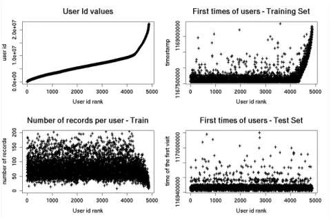
We discovered (fig. 2) a group of users (the highest id numbers) which were new to the recording system at the end of the training dataset. Interestingly, the id number growth in this group is both higher and almost constant what makes it homogeneous (fig. 2, top-left). Since we believe that the user numbers must be assigned in some natural (perhaps, chronological) order, this may mean that this group of users is distinct.
No such a group was found in the testing set.
Having had inspected the data, we henceforth assumed that the timestamp attribute represented the number of seconds passed since the beginning of the era,2i.e. 01/01/1970.
1
All the data was encoded by the contest organisers so that users, categories, etc. were represented by arbitrary numbers.
Figure 2. The users with the highest id number value were ‘newcomers’ in the training set. The testing set did not contain users with analogous property.
The timestamp range was the following:
• training set: 31/12/2006 - 22/01/2007 (finished about 1 am),
• testing set: 22/01/2007 - 31/01/2007 (finished about 1 pm).
Thus, the testing set was a chronological continuation of the training set (with less than 1 minute break in between). This chronological relationship was taken into account while selecting our prediction models. It also encouraged the authors to apply the time-series approach.
We next transformed the timestamp attribute to the full date (i.e.year,month,month-day,week-day,
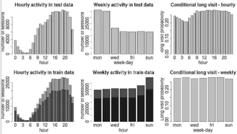
hour, minute, second) to explore the week-periodicity and 24-hour-periodicity in users’ behaviour, among others. Results are presented on figure 3.
The difference between the two histograms of week-day-based activity (fig. 3, the middle column) is due only to more Mondays and Tuesdays in the testing set and the outstanding Web activity on the Sunday, 31st December 2006, perhaps due to the New Years Eve greetings traffic, etc.3 Thus, week-day is not a good discriminant at the global level. In contrast, the hour attribute seems to bring valuable discriminative information even on the global level (see fig. 3, left column and the top right histogram).
The analysis concerning the visit length (in the context of task 1) is summarised in Table 1. One can see that short vists constitute a prevailing class.
Next, the following analysis was made in the context of tasks 2 and 3 of the challenge.
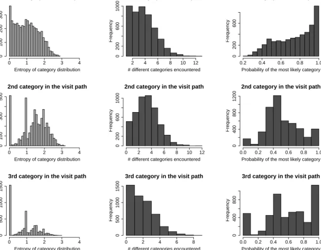
For each session in the training set, we recorded the category on the first three positions of the visit path. Subsequently, the above data was aggregated over separate users and, for each user, three 20-dimensional distribution vectors over categories were computed – for the 1st, 2nd and 3rd category on
Figure 3. Periodicity analysis. For the training set, the shorter bars represent the sessions in which more than 1 category of pages was visited, the longer bars - the other cases (task 1 of the challenge). One can observe (the histograms on the left, and top-right) that hour brings more information that week-day (almost flat bottom-right conditional histogram), on the global level.
the visit path (e.g. if a particular user visited only category 12 and 8 on the first position of their session with equal frequency, the corresponding 1st-category distribution vector has entries of 0.5 on positions 8 and 12 and values of 0 elsewhere).
Subsequently, those probability distribution vectors served as the basis for computing entropy (left column on fig. 4), number of non-zero entries (the middle column) and the probability of the most likely category on the position 1, 2 or 3, for a given user (the right column on the figure).
All those measurements served to convince us that simple, user-level model for tasks 2 and 3 is a reasonable solution. Namely, the graphs on Figure 4 clearly show, that for most of the users the categories on their 1st, 2nd and 3rd positions are quite easily predictable.
Namely, low entropy, low number of categories encountered on the first three positions and generally very high probability of the most likely category on any of the first three positions may be interpreted as
Table 1. Statistics concerning the visit length – i.e. the number of consecutive page categories visited in each ses-sion. The distribution is extremely right-skewed. The number of recorded visited categories seems to be artificially cut at the value of 200 (it was clearly visible on one of our histograms not included here)
one category two categories three categories four+ categories
72.9% 11.5% 6.3% 9.25%
Min. 1st Qu. Median Mean 3rd Qu. Max.
the fact that predicting the first three visited categories (first competition task out of the three) is not a very hard problem according to given data.
In particular, one can observe from the fig. 4 that especially categories on the 1st and 3rd positions seem to be easily predictable. The phenomenon of the 2nd category being much harder to predict can be explained with our observation that in 74.5% of the sessions of over 2 categories the third category was the same as the 1st category.
The above observations remarkably influenced our decision of choosing simple and very fast predic-tion methods.
1st category in the visit path
Entropy of category distribution
Frequency 0 1 2 3 4 0 100 200 300
1st category in the visit path
# different categories encountered
Frequency 2 4 6 8 10 12 0 200 600 1000
1st category in the visit path
Probability of the most likely category
Frequency
0.2 0.4 0.6 0.8 1.0
0
200
600
2nd category in the visit path
Entropy of category distribution
Frequency 0 1 2 3 4 0 100 300 500
2nd category in the visit path
# different categories encountered
Frequency 0 2 4 6 8 10 12 0 200 600 1000
2nd category in the visit path
Probability of the most likely category
Frequency 0.0 0.2 0.4 0.6 0.8 1.0 0 400 800 1200
3rd category in the visit path
Entropy of category distribution
Frequency 0 1 2 3 4 0 500 1000 1500
3rd category in the visit path
# different categories encountered
Frequency 0 2 4 6 8 0 500 1000 1500
3rd category in the visit path
Probability of the most likely category
Frequency
0.0 0.2 0.4 0.6 0.8 1.0
0
400
800
Figure 4. Analysis focused on assessing feasibility of user-level simple modelling for the Task 2 and 3. Row number corresponds to the position on visit path. Left column: entropy of 20-dimensional probability distribution over categories – notice its relatively low values (maximum entropy for 20-dimensional distribution is 4.32193). Middle column: number of different categories on a given position (notice that it is close to 1). Right column: data-estimated probability of the most likely category on a given position (most of the mass is definitely above the value of 0.5, except the 2nd category)
4.
Basic Concepts of the Statistical Decision Theory
Our final solutions are based on the statistical decision theory [25, 7] and learning theory [10, 13]. In this section, we briefly remind the basic concepts.
In theprediction problem, the aim is to predict the unknown value of an attributey(calleddecision attribute,outputordependent variable) of an object using known joint values of other attributes (called
condition attributes, predictors, orindependent variables) x= (x1, x2, . . . , xn). The task is to find a
functionf(x)that predicts the value ofyas accurately as possible. To assess the goodness of prediction, theloss functionL(y, f(x))is introduced for penalising the prediction error. Sincexandyare random variables, the overall measure of the classifierf(x) is the expected lossorrisk, which is defined as a functional:
R(f) =E[L(y, f(x))] =
Z
L(y, f(x))dP(y,x) (1)
for some probability measureP(y,x). The optimal (risk-minimising) decision function is:
f∗ = arg min
f R(f). (2)
SinceP(y,x)is unknown in almost all the cases, one usually minimises theempirical risk, which is the value of risk taken from the set of training examples{yi,xi}N1 :
Re(f) = 1 N N X i=1 L(yi, f(xi)). (3)
Functionf is usually chosen from some restricted family of functions.
When solving the contest tasks, the problem was to find the best approximation of the optimal deci-sion function.
5.
Solutions to the Task 1
The task is to predict whether a visit has page views of only one category (short visit), or more categories (long visit). We deal here with two classes, thus it is a simple binary classification problem for which the most common loss function is so called0-1 loss:
L0−1(y, f(x)) =
(
0 ify=f(x),
1 ify6=f(x). (4)
Coding short visit by -1 and long visit by 1, the optimal decision function for a givenxis:
f∗(x) =sgn(Pr(y= 1|x)−0.5). (5)
Of course, we have no information about the probabilitiesPr(y = 1|x), so they must be estimated from the training examples (alternatively, one can estimate whether the probability is higher or smaller than 0.5).
5.1. Shrinkage
Letp(ˆx)be an estimator of the probabilityPr(y= 1|x)(denoted asp(x)from this moment on), which is calculated on the dataset. Our objective is to find the decision function defined as:
ˆ
f∗(x) =sgn(ˆp(x)−θ) (6)
where, comparing with (5), we used the estimatorp(ˆx) instead of real unknown probability p(x) and thresholdθinstead of0.5. The motivation for the latter is based on Bayesian inference. Suppose that we impose some prior distributionτon parameterp(x). It is easily seen from the data thatEτp, the expected
value ofpaccording to the prior distributionτ, is much less then 0.5, since in 73% of the cases the visit is short. It is a well known fact from Bayesian decision theory that the estimated parameters are shrunk towards the center of prior distribution. We impose such shrinkage by introducing regularised estimate of the probability defined as:
˜
p(x) =αp(ˆx) + (1−α)Eτp,
whereαis chosen to be independent ofxfor simplicity. But the conditionp(˜x) ≥ 0.5is equivalent to the conditionp(ˆx)≥θwhere:
θ= 1 α0.5 +
α−1 α Eτp,
and θ > 0.5 as long as Eτp < 0.5. Unfortunately, as the probability distributions are unknown, θ
cannot be derived from theoretical considerations. Instead, we choose θ empirically to maximise the performance on the testing set. This is done by calculating the accuracy of the classifier on the validating set for various values ofθand doing a line-search procedure to find the maximum. The procedure is quite fast, because once we estimated the probabilitiesp(ˆx)and obtained the number of long and short visits on the testing set for each user, the calculation of accuracy is linear in the number of users. Moreover, we need to test the accuracy only for particular values ofθ, i.e. for values of the formp(ˆ x), because only then we observe any changes in classification of the objects from the testing set.
The crucial thing in estimatingp(x)is the chosen vector of predictors (condition attributes)x. De-pending on the choice of granularity, various models are possible.
5.2. Granularity
The property which is apparent in the collected dataset is its granularity. The finer granule concerns a single visit (visit’s granule), while the coarser granule corresponds to a single user (user’s granule). On the one hand, using visit’s granules permits the classifier to evaluate each visit separately, possibly giving different responses in each case, e.g. depending on the position of the visit in chronological order, timestamp, etc. On the other hand, for user’s granules we are able to do the averaging over all the visits for a given user, thus reducing the variance and giving more reliable responses.
5.3. Simple Global Model
Our first attempt was related to visit’s granules. We considered the global model, in which we divided the original training set into 2 parts: training 89% and testing 11%. The division reflected the chronological relationship between the original training and testing sets. The first 89% of the recorded sessions for
each user constituted the training subset, and the last 11% the testing subset. To train the classifiers, we used features such as user data (country,region,city,system, etc.), week day, hour, part of the day, time from the last visit, number of visits during the day, number of visits in last 60, 120, etc. minutes, type of a last visit (whether it was a short or long visit), type of a second last visit, etc.
The best result for task 1, which we achieved with the j48 algorithm4, was 75.7% correctly classified visits. We did not find these results as satisfactory and continued our work with other models.
5.4. Enhanced Global Model
Driven by the aim of improving the prediction accuracy of the results of the simple global model, we decided to estimate some additional values describing the behaviour of the users. In order to achieve it, we prepared an estimation set isolated from the training set. To reflect the chronological relationship present in data, the first 70% of the recorded sessions for each user constituted the estimation subset, the next 19% – the training subset, and the last 11% – the testing subset.
The features calculated on the estimation set belonged to a couple of different groups of attributes, as follows:
• category-based (210 attributes in total): average number of pages seen in a session, average number of groups seen each session, number of different categories seen each session, majority category at position 1 through 3 on the path, average number of pages on each position (1st through 3rd), average number of pages seen in each category, average number of groups of each category, dis-tribution of categories encountered on the 1st-3rd position of the path for each category, average number of pages seen in the 1st-3rd position for each category.
• visit-length-based, obtained by considering only two types of visits (short or long) and estimating the probability of long visit for each day of week, for each hour of working day and hour of weekend day. Probability estimates were smoothed using the kernel estimation method (Gaussian kernel).
• user-based provided with the datasets (country, region, etc. - 7 attributes in total) were also included in the dataset.
• time-based, such as the hour and week-day
Notice that all the above groups of attributes except the last one represent some average characteristics of each user so that they are related to user’s granularity level.
We experimented with taking subsets of the above attributes. We also experimented with taking logarithms of some of the above attributes (those which were extremely right-skewed).
In this setting, for the task 1, the best results were obtained with the j48 algorithm. The result was 76.7% correctly classified visits.
5.5. User Models
In the previous approach, the information about the users was incorporated into the model by isolating the estimation set (including most of the observations) and calculating some coefficients for each user
by averaging over their visits. In our next approach, we decided to usedirectlyuser id number (attribute
user id), without extracting any additional information about the users. This approach has been verified to be the most successful for all the tasks. Here we present common features of all the models.
Incorporatinguser idnumber as a condition attribute leads to the following problem:user idhas nominal scale without any order between the values, so that each value must be treated separately. It is possible to include such attribute in a general model, but for most of the classifiers, it will be binarised, i.e. changed into 4882 (number of users) binary attributes. Taking into account the size of the dataset, this is not a practical solution. Much more practical procedure, which can simulate conditioning onuser idattribute, corresponds to building a separate model for each user. Such a procedure has been used in all of the models described later.
In each of the modelsuser idnumber is used as one of the predictors (condition attributes). How-ever, in none of the models any other attributes of the user (country,region, etc.) are included. This is due to the fact, that those attributes functionally depend onuser idnumber, or in other words,user idnumber determines values on those attributes. Thus, they do not introduce any additional information, or in other words, they do not lead to finer granulation.
5.6. User Model I: Simple Classification
The only predictor isuser idnumber, so thatx≡j, wherejis the number (id) of user. For each user
j, the fraction of the long visits was taken to be a probability estimator p(j)ˆ , which is the maximum likelihood estimate of the probability. This estimator is constant in all observations for a given user. Therefore, it is characterised by a very small variance, but also a significant bias. The time complexity of the algorithm is linear with the number of visits. The memory complexity is linear with the num-ber of users (not including the memory occupied by the dataset). Once the classifier has been trained, classification of the objects is done in constant time, simply by doing a single call to the look-up table containing probability estimates.
The greatest advantage of the algorithm is its simplicity and speed. The drawback of the algorithm is that it neglects information about the timestamps of visits and their chronological order.
5.7. User Model II: Trend prediction
Data for each user was regarded as a short time series with values 0 (short visit) or 1 (long visit). The abscissa values (predictors) were timestamps of the observations (normalised, in order to avoid some numerical difficulties due to large numbers). For each user, a polynomial trend was fitted to the time series and was used as a probability estimator. The fitting procedure was regularised least squares (ridge regression). The amount of regularisation was chosen empirically, to maximise the performance of the procedure on the validation set. It appears that models with very strong regularisation (more smoothing) are preferred due to their small variance.
For a given user, the time complexity of the method is dominated by the least squares fitting which is done by Cholesky decomposition and has complexityO(m3+ nm22), wherenis the number of visits for a given user andmis the degree of the fitted polynomial. Sincemis fixed, time complexity is linear in the number of visits as well as the memory complexity. While classifying new objects, the time is constant, because it depends only onm.
5.8. User Model III: Auto-regression
The auto-regressive model was the most sophisticated one that we used. For each user a separate linear model is fitted to the user’s time series, based on the following attributes: normalised timestamp, time from the last visit, length of the last visit, average length of the last 2, 4 and 8 visits. Such attributes were chosen after testing the performance of the algorithm on the validation set for several sets of attributes. Since the predicted value (length of the current visit) depends on the values in previous moments, such algorithm resembles auto-regressive models used in time series analysis [12], but with regularised least squares fitting procedure.
The classification procedure is more complicated here – all the objects must be classified chronolog-ically, since the current value depends on the previous values. This causes the model to be less reliable with predicting the latest observations. That is why strongly regularised models (more smoothing, less variance) were preferred.
The complexity of the method, both in time and memory, is the same as for model II (linear in the number of visits), since least squares are also used as fitting procedure. However, training the auto-regressive model takes more time due to the greater number of condition attributes.
6.
Performance Comparison of All the Approaches to the Task 1
In this section, we summarise all the experimental results obtained for all our approaches to solving the Task 1 of the competition.
6.1. Configuration of Experiments
We start with a short presentation of the most important parameters of the experimental setup.
6.1.1. Estimation measures
For all our models, we considered the 3 following estimation measures:
1. Training score– value of the score on the training set. This estimate is thus over-optimistic, since the score is measured on the data which were used for fitting the classifier,
2. Validation score– the training set was divided into 89% proper training set and 11% validation set. The classifier was learnt on the proper training set and the score was calculated on the validation one. This estimate was used to choose the best classifier for the contest,
3. Solution score– value of the score on the testing set. We were able to calculate this estimate using the correct solution (actual observed visit lenghts) sent by the contest organisers after finishing the contest. The classifier was learnt on the whole training set.
6.1.2. Choice of the Threshold Value
For our models, the best value of the thresholdθwas found to be0.55. This value was obtained by the line-search procedure, which was done in the range of values between0.5and0.6.
6.1.3. Time Measurement
We also present computational time for each classifier. The times of computations reported in Table 2 are measured for a single PC machine with 512MB RAM and 2.13GHz Athlon processor. The reported time includes training and classification of the testing set, and does not include reading the training and testing files from disk into memory5.
6.2. Experimental Results
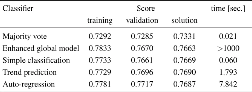
The performance results of all the our approaches to solving the Task 1 discussed earlier are reported in Table 2. The value of the score is the accuracy of the classifier, i.e. the fraction of the correctly classified observations.
To provide a baseline for the reported figures, we also included a basic ‘majority vote’ classifier which always assigns values from the larger class6. Results of this classifier coincide, of course, with values presented in Table 1).
6.3. Discussion
The presented figures do not vary greatly between the considered models, and the differences might be not statistically significant in some cases. However, because one of the goals of the research presented in this article was to compete in the contest, we treated the absolute performance figures obtained for the particular data provided by the organisers as the ultimate measure of quality of the examined approaches. We recall the best result obtained on enhanced global model by j48. As one can see, this approach is extremely time consuming (more than 1000 seconds). The result on a validation set is only slightly better than the result of the simplest user model. We expected a weak stability of the generated tree and worse accuracy on the testing data. This model has also, as one could expect, the best (but overestimated) accuracy on training data. However, this model, as one could expect, achieved lower solution score than other considered models (except the baseline model) including the simple classification model.
Notice that although regression results were sent for the contest (the highest validation score), the best results on the testing set were achieved by the trend prediction approach (the highest solution score). All the user models were relatively fast, especially simple classification. Also all the user models, have very similar results (almost no change in the score value). This suggests that any other condition attributes based on timestamp or previous visit length are hardly informative. This would also suggest choosing the simplest (parsimonious) model which is simple classification. We also noticed that in case of more complicated models (trend prediction and regression), a strong regularisation was preferred in order to decrease the complexity of the model and reduce variance.
In comparison to the global models, all the user models got better solution score. This is due to the fact that the user models are simpler (less attributes taken into account), more stable, easier in parameter-isation, and for these reasons, much more faster. The advantage of user models over the global models in the context of accuracy, comes from the fact that user models employuser iddirectly. Global models use some surrogate, such as attributes of the users (country,region, etc.) and statistics of the user, which are less informative. In fact, by investigating the results of the global models, we came to the
5
It took additional6.409seconds for the mentioned machine
Table 2. Comparison of the performance of all the examined approaches to the task 1 of the competition. The figures represent the accuracy of the classifier for three different subsets of the annotated data. The solution dataset was provided by the organisers after the competition completed. The last column gives some insight into the efficiency of the considered approaches (the experiments were performed on a single standard PC).
Classifier Score time [sec.]
training validation solution
Majority vote 0.7292 0.7285 0.7331 0.021 Enhanced global model 0.7833 0.7670 0.7663 >1000 Simple classification 0.7733 0.7661 0.7669 0.060 Trend prediction 0.7729 0.7696 0.7690 1.793 Auto-regression 0.7781 0.7717 0.7687 7.842
conclusion that as more user attributes and statistics are given to the classifier, its accuracy approaches the accuracy of the user models.
The only problem with the user models is the so calledcold start problem, i.e. the poor performance of the learning algorithms when the amount of information about the user is small. For instance, if a new user enters the dataset, the best thing we can do is predicting the visit length using the a priori distribution ofp(x), i.e. predicting the visit length to be short. On the other hand, global models are less prone to the cold start problem, because the user attributes are immediately available from the first visit of the user; however, the statistics of the user, used in the enhanced global models, are also unknown. Taking into account all the pros and cons, we conclude that the user models seem to be generally a better choice if we ignore the ‘cold start’ problem.
7.
Solutions to the Tasks 2 and 3
In this section we present our solutions to the remaining contest tasks.
7.1. Solution to the Task 2
The second task concerns predicting a list of the 3 most probable categories (i.e. the first three page categories on the visit path) during a given visit of a given user. A specific score function was defined by the organisers in order to quantitatively measure the quality of prediction.
Assume thaty= (y1, . . . , ym)is a sequence ofmvisited categories. Moreover letf(x) = (f1(x), f2(x), f3(x))
be the sequence of the3most probable categories predicted by the classifier based on some predictor vec-torx. According to the challenge rules, if the same category is present on both the 1st and the 3rd position ofyandf(x), we assume that it is regarded as a new, different category.
The organisers of the competition defined an arbitrary score function to quantitatively measure and compare the solutions to the task 2. According to this, we defined our loss function as the negative of the
provided score function, which can be written in the following way: L(y, f(x)) =− m X j=1 3 X k=1 s(j, k)I(yj =fk(x)) (7) where s(j, k) = max{1,min{6−j,6−k}} (8) is the single score value andI(x)is the indicator function equal to1ifxis true,0otherwise. The risk of the classifier has the following form:
R(f) =
Z X
y
L(y, f(x))P(y|x)dP(x) (9)
In order to find the optimal decision for a fixed predictor x, we must minimise the risk point-wise, i.e. minimise P
yL(y, f(x))P(y|x). Since the probabilities P(y|x) are unknown, we use empirical risk
minimisation (3), so that we minimise the loss function (7) on the dataset. However, one can show, that estimating the probabilitiesP(y|x)by frequencies would lead exactly to the same result.
Thus, the optimal decision function is obtained simply by choosing for each value x, f(x) = (f1(x), f2(x), f3(x))which minimises the empirical risk. However, one does not need to go through
the whole dataset for each combination of values of f(x). It is enough to calculate three aggregated coefficients for each category for a given x and then choosing f(x) is independent of the number of visits.
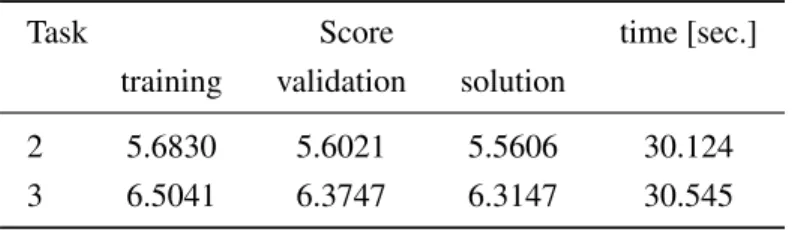
There is stillxto be chosen to make the model complete. Motivated by our exploratory analysis (see section 3) and the results for task 1, we decided to use parsimonious model taking into account only one predictor -user idnumber. Thus, the classifier is constant on every visit of the same user, so that it corresponds to user’s granulation described in section 5.2. In other words, the user model was chosen. Such model has the advantage of being stable and having small variance. The results obtained using the model are presented in Table 3. They indicate that the model, despite its simplicity, has fairly good accuracy.
The time complexity of the method is linear with the number of visits. The memory complexity is (not including the dataset itself) linear with the number of users. Classifying new objects is constant in the number of visits and users.
We did not perform tests on the global models, because it was shown in section 5, that their perfor-mance is inferior to the user models. Moreover, it would be very hard to minimise the complicated score (7) within a restricted class of functions (trees, linear functions, etc.), whereas each global model uses such restriction to train the classifier.
7.2. Solution to the Task 3
The third task was an extension of the second task. Apart from giving a list of the most probable cat-egories in a visit, it concerns giving a range of number of page views in each category. Assume that
y= ((y1, t1), . . . ,(ym, tm))is the sequence ofmvisited pairs (category,#pages range) and
Table 3. Performance of the risk minimisation approach chosen to solve the tasks 2 and 3 on the three different subsets of the dataset (as in Table 2). The figures represent the average value of the arbitrary score function defined by the organisers.
Task Score time [sec.]
training validation solution
2 5.6830 5.6021 5.5606 30.124 3 6.5041 6.3747 6.3147 30.545
is the sequence of the 3 most probable pairs (category, #pages range) predicted by the classifier based on some predictor vectorx. Similarly as in the case of task 2, we defined our loss function as the negative value of the arbitrary score function provided by the competition organisers, which can be written as follows:7 L(y, f(x)) =− m X j=1 3 X k=1 s(j, k)I(yj =fkc(x)) +I(tj =fkt(x)) (10)
Similarly as in the case of task 2, we minimised the empirical risk (3) to obtain the decision function. Again, only one predictorxwas chosen –user idnumber.
The final results obtained for tasks 2 and 3 are shown in Table 3. The time and memory complexity of the method is the same as for the task 2.
The choice of the user model and discarding the global models was motivated by the arguments as in the case of task 2.
8.
Conclusions
After an intensive exploratory data analysis phase we examined various different approaches to the con-test tasks and chose the solution that is simple, but effective and theoretically well-founded. We found this choice optimal in the context of the limited time duration of the contest.
During our work, we have observed that models constructed separately for each user (user-models) give generally better results than the global ones. The reason of this is a specific nature of data and the formulation of the challenge problems. In order to obtain stable predictions, our methods are strongly based on statistical decision [25, 7] and learning theory [10, 13].
All of our algorithms scale well with large data and have linear time complexity, which is the smallest possible complexity for such problems, since reading the dataset is already linear in its size. The memory complexity never exceeds linear rate and grows linearly with the number of users, not visits. Moreover, the time complexity of classifying new objects is constant in the number of users and visits, which means that once the model has been trained, classification does not take significant time.
7
The scoring functions provided by the organisers of the competition are described in detail in the competition description, a copy of which can be found at [1]
Our final choice of the user-level approach and discarding the global models was motivated by the fact, that user models turned out to be more accurate, stable and are much faster than the global ones. The only problem with the user models is the cold start problem, i.e. as the new user enters the system, we are not able to make the ‘depersonalised’ prediction until some information about the user is gathered in the dataset.
For solving the tasks 2 and 3 we chosen a simple and fast, yet quite effective empirical-minimisation approach.
Possible further directions of the research described here would concern considering clustering the users or examining how the prediction accuracy depends on the size of the training data.
Acknowledgements
Most of the computational work was done with the extensive use of free/open-source software.
In particular, data preprocessing was done with the help of the Linux/GNU tools [3] and especially the GNU/AWK programming language.
All the graphical visualisations and all the computations concerned with the exploratory data analysis (section 3) were performed using the R package [5, 21]
The machine learning experiments were executed with the Weka package [6] as well as our custom implementations of some algorithms in Java [4].
One of the authors was supported with the Polish-Japanese Institute of Information Technology in-ternal grant ST/SI/03/2008 ‘Analysis of the Behaviour of Web users’.
References
[1] ECML/PKDD 2007 Discovery Challenge, Track 1 description (a copy),
http://www.pjwstk.edu.pl/ msyd/predicting users behaviour.pdf.
[2] Gemius S.A. Company, Warsaw, Poland,http://www.gemius.com. [3] GNU/Linux operating system and toolset,http://www.gnu.org. [4] Java programming language,http://java.sun.com/.
[5] R statistical package,http://www.r-project.org.
[6] Weka machine learning package,http://www.cs.waikato.ac.nz/ml/weka/.
[7] Berger, J.:Statistical Decision Theory and Bayesian Analysis, Springer-Verlag, New York, 1993. [8] Dasu, T., Johnson, T.:Exploratory Data Mining and Data Cleaning, Wiley, 2003.
[9] Dembczy´nski, K., Kotłowski, W., Sydow, M.: Effective Prediction of Web User Behaviour with User-Level Models, 2007.
[10] Duda, R., Hart, P., Stork, D.:Pattern Classification, Second Edition, Wiley-Interscience, 2000. [11] ECML/PKDD’2007 Discovery Challenge: User’s behaviour prediction, 2007,
http://www.ecmlpkdd2007.org/challenge/.
[13] Hastie, T., Tibshirani, R., Friedman, J.: Elements of Statistical Learning: Data Mining, Inference, and Prediction, Springer-Verlag, 2003.
[14] Hu, J., Zeng, H.-J., Li, H., Niu, C., Chen, Z.: Demographic prediction based on user’s browsing behavior,
WWW ’07: Proceedings of the 16th international conference on World Wide Web, ACM, New York, NY, USA, 2007, ISBN 978- 1- 59593- 654-7.
[15] Jaworska, J., Sydow, M.: Behavioural Targeting in On-line Advertising: An Empirical Study, 2008, Ac-cepted for the 9th International Conference on Web Information Systems Engineering (Wise 2008), Auck-land, New ZeaAuck-land, September 1-4, 2008 (to be printed in LNCS, Springer).
[16] Lee, T.-Y.: Predicting User’s Behavior by the Frequent Items, 2007.
[17] M.T. Hassan, K. J., Karim, A.: Bayesian Inference for Web Surfer Behavior Prediction, 2007. [18] Newcomb, K.: Search Marketing Shows Strength in 2006,searchenginewatch.com, 2007.
[19] Ng, V., Mok, K.-H.: An Intelligent Agent for Web Advertisements,CODAS ’01: Proceedings of the Third International Symposium on Cooperative Database Systems for Advanced Applications, IEEE Computer Society, Washington, DC, USA, 2001, ISBN 0-7695-1128-7.
[20] Quinlan, J. R.:C4.5: Programs for Machine Learning, Morgan Kaufmann, 1993.
[21] R Development Core Team: R: A language and environment for statistical computing, R Foundation for Statistical Computing, 2005.
[22] Regelson, M., Fain, D. C.: Predicting click-through rate using keyword clusters,Proceedings of the Second Workshop on Sponsored Search Auctions, 2006.
[23] Richardson, M., Dominowska, E., Ragno, R.: Predicting clicks: estimating the click-through rate for new ads,WWW ’07: Proceedings of the 16th International Conference on World Wide Web, ACM, New York, NY, USA, 2007.
[24] Smith, S.: Behavioral targeting could change the game, January, 23 2007, Available at:
http://www.econtentmag.com/Articles/ArticleReader.aspx?ArticleID=18964, accessed February 19, 2008. [25] Wald, A.: Statistical decision functions, Wiley, 1950.
[26] Witten, I., Frank, E.:Data Mining: Practical machine learning tools and techniques, 2nd Edition, Morgan Kaufmann, 2005.