Escuela Politécnica Superior
Departamento de Ingeniería Informática
Acceleration Methods for Classic Convex Optimization
Algorithms
A thesis submitted in partial fulfillment for the degree ofDoctor of Philosophy
By
Alberto Torres Barrán
under the direction of
José R. Dorronsoro Ibero
Department: Ingeniería Informática Escuela Politécnica Superior
Universidad Autónoma de Madrid (UAM) Spain
Title: Acceleration Methods for Classic Convex Optimization Algorithms Author: Alberto Torres Barrrán
Advisor: José R. Dorronsoro Ibero Date: June 2017
Committee:
• President: Aníbal Ramón Figueiras Vidal
• Secretary: Daniel Hernández Lobato
• Vocal 1: César Hervás Martínez
• Vocal 2: María Amparo Alonso Betanzos
• Vocal 3: David Ríos Insua
• Substitute 1: Ana María González Marcos
Most Machine Learning models are defined in terms of a convex optimization problem. Thus, developing algorithms to quickly solve such problems its of great interest to the field. We focus in this thesis on two of the most widely used models, the Lasso and Support Vector Machines. The former belongs to the family of regularization methods, and it was introduced in 1996 to perform both variable selection and regression at the same time. This is accomplished by adding a`1-regularization term to the least squares model, achieving interpretability and also a good generalization error.
Support Vector Machines were originally formulated to solve a classification problem by finding the maximum-margin hyperplane, that is, the hyperplane which separates two sets of points and its at equal distance from both of them. SVMs were later extended to handle non-separable classes and non-linear classification problems, applying the kernel-trick. A first contribution of this work is to carefully analyze all the existing algorithms to solve both problems, describing not only the theory behind them but also pointing out possible advantages and disadvantages of each one.
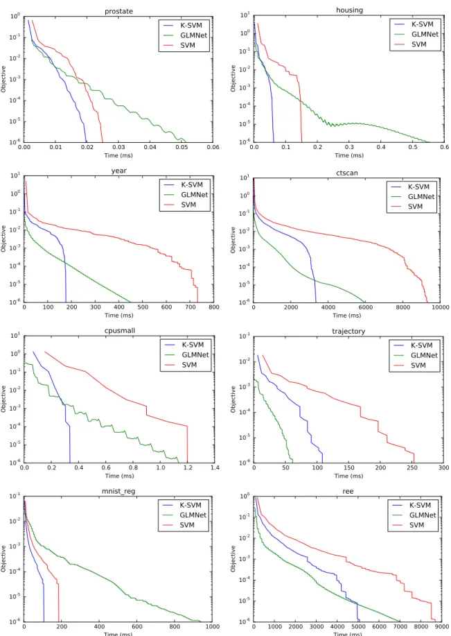
Although the Lasso and SVMs solve very different problems, we show in this thesis that they are both equivalent. Following a recent result by Jaggi, given an instance of one model we can construct an instance of the other having the same solution, and vice versa. This equivalence allows us to translate theoretical and practical results, such as algorithms, from one field to the other, that have been otherwise being developed independently. We will give in this thesis not only the theoretical result but also a practical application, that consists on solving the Lasso problem using the SMO algorithm, the state-of-the-art solver for non-linear SVMs. We also perform experiments comparing SMO to GLMNet, one of the most popular solvers for the Lasso. The results obtained show that SMO is competitive with GLMNet, and sometimes even faster.
Furthermore, motivated by a recent trend where classical optimization methods are being re-discovered in improved forms and successfully applied to many problems, we have also analyzed two classical momentum-based methods: the Heavy Ball algorithm, introduced by Polyak in 1963 and Nesterov’s Accelerated Gradient, discovered by Nesterov in 1983. In this thesis we develop practical versions of Conjugate Gradient, which is essentially equivalent to the Heavy Ball method, and Nesterov’s Acceleration for the SMO algorithm. Experiments comparing the convergence of all the methods are also carried out. The results show that the proposed algorithms can achieve a faster convergence both in terms of iterations and execution time.
La mayoría de modelos de Aprendizaje Automático se definen en términos de un problema de optimización convexo. Por tanto, desarrollar algoritmos para resolver rápidamente dichos problemas es de gran interés para este campo. En esta tesis nos centramos en dos de los modelos más usados, Lasso y Support Vector Machines. El primero pertenece a la familia de métodos de regularización, y fue introducido en 1996 para realizar selección de características y regresión al mismo tiempo. Esto se consigue añadiendo una penalización`1al modelo de mínimos cuadrados, obteniendo interpretabilidad y un buen error de generalización.
Las Máquinas de Vectores de Soporte fueron formuladas originalmente para resolver un problema de clasificación buscando el hiper-plano de máximo margen, es decir, el hiper-plano que separa los dos conjuntos de puntos y está a la misma distancia de ambos. Las SVMs se han extendido posteriormente para manejar clases no separables y problemas de clasificación no lineales, mediante el uso de núcleos. Una primera contribución de este trabajo es analizar cuidadosamente los algoritmos existentes para resolver ambos problemas, describiendo no solo la teoría detrás de los mismos sino también mencionando las posibles ventajas y desventajas de cada uno.
A pesar de que el Lasso y las SVMs resuelven problemas muy diferentes, en esta tesis demostramos que ambos son equivalentes. Continuando con un resultado reciente de Jaggi, dada una instancia de uno de los modelos podemos construir una instancia del otro que tiene la misma solución, y viceversa. Esta equivalencia nos permite trasladar resultados teóricos y prácticos, como por ejemplo algoritmos, de un campo al otro, que se han desarrollado de forma independiente. En esta tesis mostraremos no solo la equivalencia teórica sino también una aplicación práctica, que consiste en resolver el problema Lasso usando el algoritmo SMO, que es el estado del arte para la resolución de SVM no lineales. También realizamos experimentos comparando SMO a GLMNet, uno de los algoritmos más populares para resolver el Lasso. Los resultados obtenidos muestran que SMO es competitivo con GLMNet, y en ocasiones incluso más rápido.
Además, motivado por una tendencia reciente donde métodos clásicos de optimización se están re- descubriendo y aplicando satisfactoriamente en muchos problemas, también hemos analizado dos métodos clásicos basados en “momento”: el algoritmo Heavy Ball, creado por Polyak en 1963 y el Gradiente Acelerado de Nesterov, descubierto por Nesterov en 1983. En esta tesis desarrollamos versiones prácticas de Gradiente Conjugado, que es equivalente a Heavy Ball, y Aceleración de Nesterov para el algortimo SMO. Además, también se realizan experimentos comparando todos los métodos. Los resultados muestran que los algoritmos propuestos a menudo convergen más rápido, tanto en términos de iteraciones como de tiempo de ejecución.
First of all, I would like to thank my supervisor José R. Dorronsoro Ibero for all the help and advice during this period. I am also immensely grateful to all the professors who volunteered to come to the thesis panel and read this dissertation. I express my gratitude to Professor Johan A.K. Suykens for giving me the opportunity to join the ESAT department at KU Leuven during the research stay of 2015.
I would also like to mention all the grants and institutions that supported my research: FPU12/05163 grant, funded by “Ministerio de Economía, Cultura y Deporte”; FPI grant, funded by “Universidad Autónoma de Madrid”; “Cátedra IIC Modelado y Predicción” funded by “Instituto de Ingeniería del Conocimiento” and “Instituto de Ciencias Matemáticas” (ICMAT-CSIC). Finally, I gratefully acknowledge the computational resources provided by “Centro de Computación Científica” (CCC) at “Universidad Autónoma de Madrid”.
Abstract vii Resumen vii Acknowledgments ix Contents x 1 Introduction 1 1.1 Outline . . . 2 1.2 Contributions . . . 3 2 Mathematical background 5 2.1 Machine Learning . . . 5 2.1.1 Regression . . . 5 2.1.2 Classification . . . 7 2.1.3 Model selection . . . 8 2.1.4 Regularization . . . 10 2.2 Convex optimization . . . 12 2.2.1 Duality . . . 14 2.2.2 Subgradients . . . 15 2.2.3 Algorithms . . . 19
3 Theory and algorithms for the Lasso 21 3.1 Lasso . . . 21
3.2 Elastic Net . . . 23
3.2.1 Naïve Elastic Net . . . 25
3.2.2 General Elastic Net . . . 28
3.3 Algorithms . . . 29
3.3.1 Least Angle Regression . . . 29
3.3.2 Proximal Gradient Descent . . . 32
3.3.3 Coordinate Descent . . . 38
3.3.4 Stochastic Coordinate Descent . . . 41
3.3.5 Stochastic Gradient Descent . . . 42
3.3.6 Stochastic Dual Coordinate Ascent . . . 44
3.4 Screening . . . 47 xi
4 Theory and algorithms for Support Vector Machines 51
4.1 Support Vector Classification . . . 51
4.1.1 Hard-margin SVC . . . 51
4.1.2 Soft-margin SVC . . . 53
4.1.3 Kernel trick . . . 54
4.1.4 ν-Support Vector Classification . . . 55
4.1.5 One-class Support Vector Machine . . . 56
4.2 Support Vector Regression . . . 57
4.3 Algorithms . . . 58
4.3.1 Primal gradient methods . . . 59
4.3.2 Dual coordinate methods . . . 63
4.3.3 Decomposition methods . . . 65
4.3.4 Shrinking . . . 70
5 Relation between the Lasso and SVMs 73 5.1 Previous work . . . 73
5.1.1 Lasso to SVM . . . 74
5.1.2 SVM to Lasso . . . 75
5.1.3 Elastic Net to SVM . . . 76
5.2 Constrained and unconstrained Lasso . . . 77
5.3 Constrained Lasso to Nearest Point Problem . . . 80
5.4 Numerical experiments . . . 83
5.4.1 Implementation details . . . 84
5.4.2 Datasets and methodology . . . 85
5.4.3 Results . . . 87
5.5 Discussion and further work . . . 92
6 Accelerating SVM training 95 6.1 Nesterov Accelerated Gradient . . . 96
6.1.1 Naïve Nesterov Accelerated SMO . . . 98
6.1.2 Monotone Nesterov’s Accelerated SMO . . . 100
6.2 Conjugate Gradient Descent . . . 102
6.2.1 Conjugate MDM . . . 106
6.2.2 Conjugate SMO . . . 109
6.3 Numerical experiments . . . 113
6.3.1 MDM . . . 114
6.3.2 SMO: Algorithm correctness . . . 118
6.3.3 SMO: Iteration comparison . . . 120
6.3.4 SMO: Comparison versus LIBSVM . . . 129
6.4 Discussion and further work . . . 143
7 Conclusions 145 7.1 Discussion . . . 145 7.2 Further work . . . 147 8 Conclusiones 149 8.1 Discusión . . . 149 8.2 Trabajo futuro . . . 151
Appendices 153 A Derivation of the soft-thresholding operator 155
B Convergence rates 157
C Iteration results 159
D Published papers 167
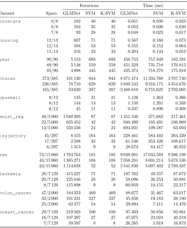
5.1 Optimalλvalues,λ/λmaxratio, sample sizes and input dimensions of the datasets considered. . . 86 5.2 Sparsity of final solutions, number of iterations and running times. . . 88 6.1 Sample sizes and input dimensions of the datasets considered. . . 114 6.2 Median of the execution times and number of iterations for all possible values of
the initial point for both standard MDM and conjugate MDM (CMDM). . . 115 6.3 Dimensions, data sizes and class sizes of the datasets considered. . . 118 6.4 Final value of SMO’s objective function and number of support vectors (nSV) for
= 0.1 and= 0.001 . . . 119 6.5 Relative error with respect to SMO in the coefficients, objective value and number
of support vectors for CS and MNAS (= 0.1) . . . 121 6.6 Relative error with respect to SMO in the coefficients, objective value and number
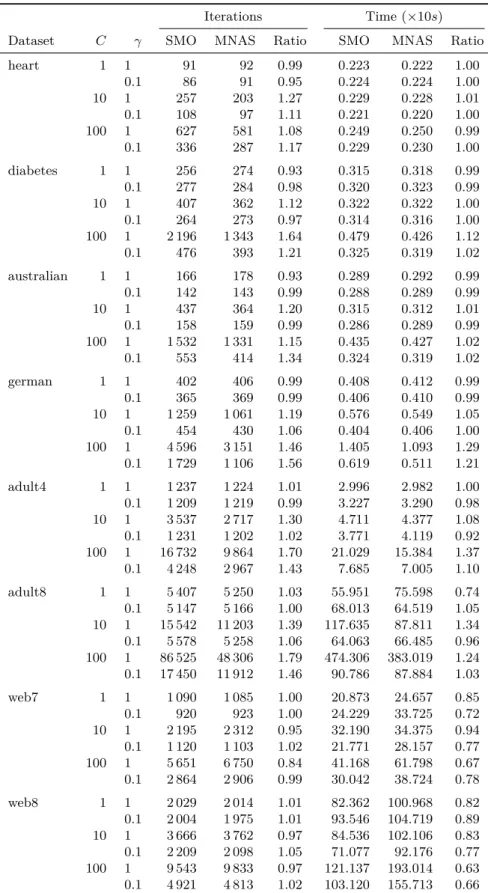
of support vectors for CS and MNAS (= 0.001) . . . 122 6.7 Number of iterations and time for SMO and Monotone Nesterov Accelerated SMO
(MNAS), together with their ratios SMO/MNAS (= 0.1) . . . 123 6.8 Number of iterations and time for SMO and Monotone Nesterov Accelerated SMO
(MNAS), together with their ratios SMO/MNAS (= 0.001) . . . 124 6.9 Number of iterations and time for SMO and Conjugate SMO (CS), together with
their ratios SMO/CS (= 0.1) . . . 125 6.10 Number of iterations and time for SMO and Conjugate SMO (CS), together with
their ratios SMO/CS (= 0.001) . . . 126 6.11 Iterations, objective value and number of support vectors for the adult9 and
web8 datasets . . . 130 6.12 Running time in seconds for the adult9and web8 datasets . . . 130 6.13 Dimensions, data sizes and class sizes of the datasets considered. . . 131 6.14 Comparison of the running time in seconds between SMO, Conjugate SMO (CS)
and Hybrid SMO (HS) for theadult8dataset . . . 133 6.15 Comparison of the running time in seconds between SMO, Conjugate SMO (CS)
and Hybrid SMO (HS) for theweb8 dataset . . . 134 6.16 Comparison of the running time in seconds between SMO, Conjugate SMO (CS)
and Hybrid SMO (HS) for theijcnn1dataset . . . 135 6.17 Comparison of the running time in seconds between SMO, Conjugate SMO (CS)
and Hybrid SMO (HS) for thecod-rnadataset . . . 136 6.18 Comparison of the running time in seconds between SMO, Conjugate SMO (CS)
and Hybrid SMO (HS) for themnist1dataset . . . 137 6.19 Comparison of the running time in seconds between SMO, Conjugate SMO (CS)
and Hybrid SMO (HS) for theskin dataset . . . 138
6.20 Relative time difference as a percentage between SMO and CS for a full hyper-parameter search with= 0.001 and a 100 Mb cache . . . 139 C.1 Comparison of the number of iterations between SMO, Conjugate SMO (CS) and
Hybrid SMO (HS) for the adult8dataset . . . 160 C.2 Comparison of the number of iterations between SMO, Conjugate SMO (CS) and
Hybrid SMO (HS) for the web8dataset . . . 161 C.3 Comparison of the number of iterations between SMO, Conjugate SMO (CS) and
Hybrid SMO (HS) for the ijcnn1dataset . . . 162 C.4 Comparison of the number of iterations between SMO, Conjugate SMO (CS) and
Hybrid SMO (HS) for the cod-rnadataset . . . 163 C.5 Comparison of the number of iterations between SMO, Conjugate SMO (CS) and
Hybrid SMO (HS) for the mnist1dataset . . . 164 C.6 Comparison of the number of iterations between SMO, Conjugate SMO (CS) and
2.1 Linear least squares fitting with X∈R. . . 7 2.2 Points are generated from a random quadratic model with Gaussian noise and
they are fitted to linear (purple line), quadratic (blue) and polynomial functions (red). Green points are also drawn from the same model but not used to fit the
functions. . . 9 2.3 Test and training error as a function of the model complexity (Hastie et al., 2003) 10 2.4 Example of convex set (left) and non-covex set (right) [Wikipedia, “Convex set”] 13 2.5 A convex function (blue) and “subtangent” lines atx0 (red) [Wikipedia
“Subdif-ferential”] . . . 16 2.6 Convex hull of a set of points . . . 16 3.1 Subset regression, Ridge Regression, Lasso and garotte shrinkage comparison in
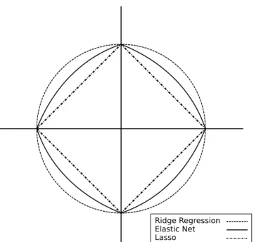
the case of an orthonormal design. . . 24 3.2 Lasso (a) and Ridge Regression (b) estimates (Tibshirani, 1994) . . . 25 3.3 Lasso, Ridge Regression and Elastic Net penalties for the two variable case . . . 26 3.4 Convergence of ISTA and FISTA . . . 37 4.1 Linear Support Vector Regression (left) and -insensitive loss (right). Support
vectors are drawn with a black outline (Yu et al., 2014) . . . 57 4.2 Support Vector Machines loss function (hinge loss) compared to the logistic
regression loss (negative log-likelihood loss). They are shown as a function ofyf
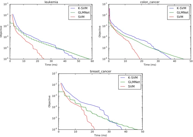
rather than f because of the symmetry between the y = +1 and y = −1 case (Hastie et al., 2003). . . 60 5.1 Geometrical interpretation of problem (5.3.2) . . . 81 5.2 Time evolution of the objective function for the three classification datasets with
λ∗ as the penalty factor . . . 89 5.3 Time evolution of the objective function for the eight regression datasets with λ∗
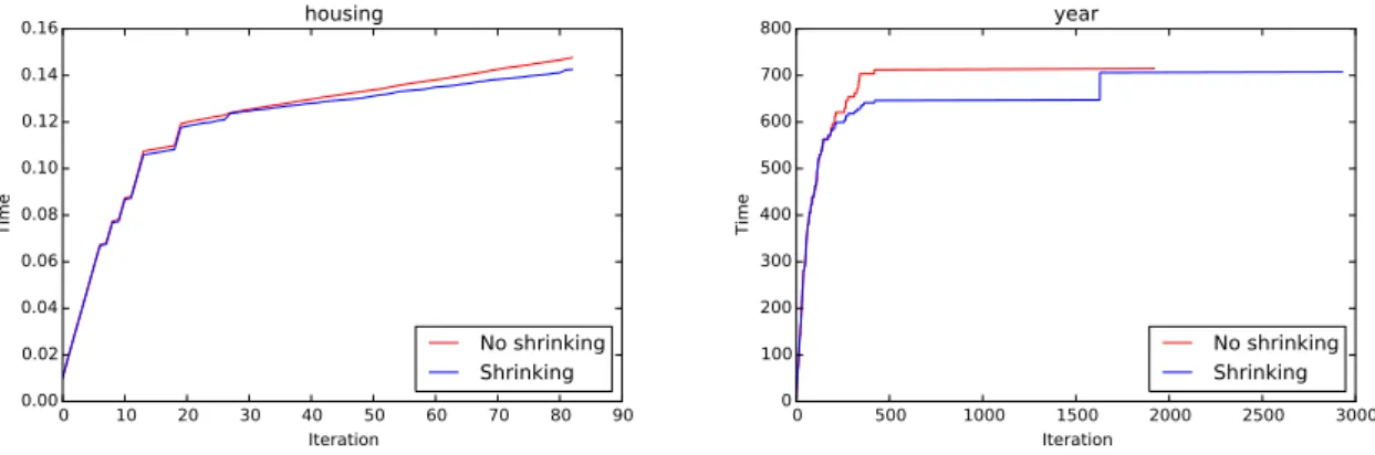
as the penalty factor . . . 90 5.4 Time versus iterations for thehousingandyeardatasets with penalty 2λ∗ with
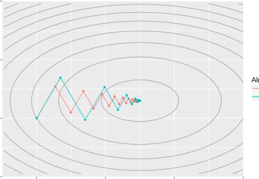
and without shrinking . . . 91 6.1 Convergence of Gradient Descent (GD) and the Heavy Ball (HB) methods for the
optimal choices ofη andβ. . . 104 6.2 Convergence of Gradient Descent (GD) and the Heavy Ball (HB) methods for
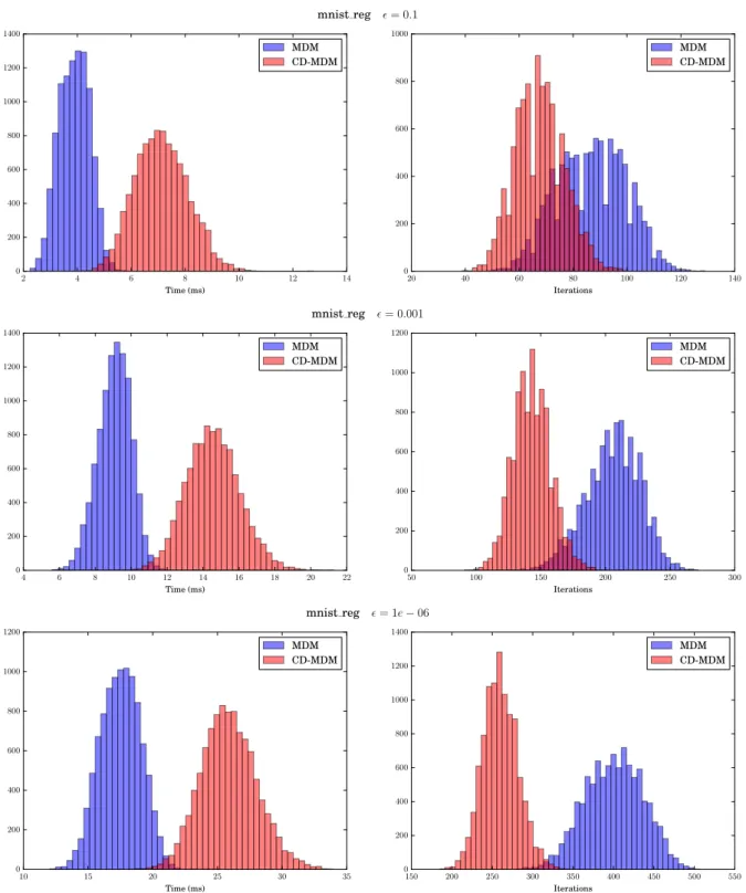
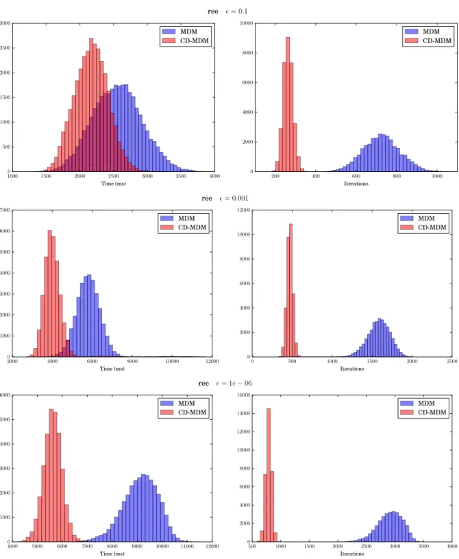
η= 0.18 and β= 0.3. . . 105 6.3 Execution times and iterations histograms for the dataset mnist_regand
toler-ance= 0.1,= 0.001 and= 1e−06. . . 116 xvii
6.4 Execution times and iterations histograms for the dataset ree and tolerance
= 0.1, = 0.001 and = 1e−06. . . 117 6.5 Evolution of the number of iterations with respect toC for the eight datasets . . 127 6.6 Evolution of the objective function with = 0.001 for theadult4(top) and the
web7datasets . . . 128 6.7 Time evolution of the objective function (left) and number of kernel operations
(right) for different cache sizes. . . 129 6.8 Comparison between SMO and CS of the running time as a function of the cache
size for theadult9 and web7datasets and different C values . . . 132 6.9 Relative time difference heatmap with a cache size of 100 Mb (a) . . . 140 6.9 Relative time difference heatmap with a cache size of 100 Mb (b) . . . 141 6.10 Relative time difference heatmap with a cache size of 100 Mb for the differentC
and γ values of a full hyper-parameter search . . . 142 B.1 Comparison of sublinear (1/k and 1/k2), linear and superlinear (quadratic)
1 ISTA with constant stepsize . . . 34
2 ISTA with backtracking . . . 35
3 FISTA with constant stepsize . . . 35
4 FISTA with backtracking . . . 36
5 Cyclic Coordinate Descent (CCD), naive updates . . . 39
6 Cyclic Coordinate Descent (CCD), covariance updates . . . 40
7 Stochastic Coordinate Descent (SCD) . . . 42
8 Truncated Gradient Descent (TGD) . . . 43
9 Stochastic MIrror Descent Algorithm made Sparse (SMIDAS) . . . 45
10 Pegasos for the linear SVM . . . 61
11 Pegasos for the nonlinear SVM . . . 62
12 Dual coordinate descent for the Linear SVM . . . 64
13 Sequential Minimal Optimization (SMO) . . . 69
14 Naïve Nesterov’s Accelerated SMO . . . 99
15 Monotone Nesterov’s Accelerated SMO (MNAS) . . . 102
16 Conjugate MDM (CMDM) . . . 108
17 Conjugate SMO (CSMO) . . . 112
Matrices are denoted in upper-case bold font (X), whereas vectors are denoted in lower-case bold, (x). Plain font stands for scalars (x), usually lower-case, although some important scalar constants are denoted in upper-case (for instance, C). Upper-case plain font is also used for random variables (X). Sets are usually denoted by calligraphic font (X) and spaces with blackboard bold font (R). Components of a vector are denoted in subscript (xi); when the component is another sub-vector the bold face is mantained (xi). The components of a matrix X are denoted by two subscripts (Xi,j). A single subscript on a matrix may indicate both the vector corresponding to a single row or column (Xi). This is indicated when it is not clear by the context. For a general sequence brackets are employed ({xk}) and element of such sequences are denoted in superscript (xk). A superscript∗ indicates the limit of a sequence, such as the optimum (x∗).
All the non-standard operators are defined on their first use. Regarding the standard ones, kxk indicates the norm of a vector x, ∇ is used for the gradient and x·y denotes the inner product between vectorsx and y. The inner product is sometimes also written as x>y. The transpose of a matrix isX> and its inverse X−1. ∂ stands for both the partial derivative and the subdifferential, and it should be clear from the context which is which. The standard big O notation is written asO(·).
Introduction
Machine learning is a branch of artificial intelligence commonly defined as the science of learning from data without the need for the computer to be explicitly programmed. Other fields that overlap with machine learning are statistics, data mining and pattern recognition, since they often use the same methods. Some example of learning problems are:
• Learn to distinguish between spam and non-spam email messages and classify new messages accordingly.
• Predict the selling price of a house based on facts such as square meters and number of bedrooms.
• Predict the price of a stock in 6 months from now, on the basis of company performance measures and economic data (Hastie et al., 2003).
• Recognize handwritten digits from a digitized image, for example ZIP codes in letters. • Identify the risk factors for prostate cancer, based on clinical and demographic variables
(Hastie et al., 2003).
• Identify the clients of an insurance company who are likely to upgrade their policy to premium if an offer is made to them.
In the typical scenario we have an outcome measurement we want to predict, which can be either quantitative (price of the house) or categorical (spam/non-spam), based on a set of features or variables. We have a set of data, in which we observe both the features and the outcome, and the goal is to build a prediction model which allows us to predict the outcome of new samples, not used to train the model.
Notice that it is impossible to compute the accuracy of the predictions for the new data, since the real outcome is not available. So, in order to asses the quality of the model, the original dataset is usually divided into a training set and a test set. The former is used to build the prediction model while the latter is used to estimate its performance. This is done by computing the accuracy of the predictions in the test set and, since they were not used for training, they are a good estimate of the accuracy for new data (assuming they aresimilar).
The ability to predict correctly the outcome of new unseen data is known as generalization. In practice the variability of the data will be such that the training set can comprise only a small amount of all possible examples, so generalization is a central goal in machine learning.
Machine learning systems also have to deal with the representation of the data. For instance, in the case of handwritten digits recognition, it is usually convenient to represent the digitized
images as numerical vectors using a greyscale approach. Data is also usually pre-processed to transform it into another space where the problem of building the model is easier to solve. Continuing with the example of digit recognition, the images are typically traslated and scaled so that each digit is contained in a fixed size box (Bishop, 2007). Note that new data must be processed using the same steps as the training data.
So far we have only mentioned the task where the training data contains both the features and the outcome. That kind of data is said to be labeled, and such applications are known as
supervised learning problems. These problems can be further divided into classification, if the outcome is a finite number of discrete categories, orregression, if the outcome consists of one or more continuous variables. Examples of classification problems are spam detection, handwritten digits recognition and identifying possible premium users. Examples of regression problems are house pricing, prostate cancer detection and stock price prediction.
There are other machine learning problems where the input data consists only of features, and no outcome is available. In those unsupervised learning problems the goal is to find some kind of structure in the data: groups of similar examples (clustering), distribution of the data in the input space (density estimation) or subspaces in which the data is still “meaningful” but with less dimensions (dimensionality reduction).
1.1
Outline
The rest of thesis is organized as follows:
1. Chapter 2 contains the necessary mathematical background to understand this thesis: learning theory, where we include examples of the simplest linear models, and the basics of convex optimization. We skip and therefore assume the reader is familiar with basic results in linear algebra and probability theory.
2. Chapter 3 presents a detailed review of the theory behind the Lasso model and the different optimization algorithms that exist in the literature to solve it. The sparsity of the Lasso regularization was exploited in Alaíz et al. (2012) and Torres et al. (2014b).
3. Chapter 4 is analogous to Chapter 3 but regarding the SVM model. We will address the formulation of the different variants and the different methods used to optimize them. The generalization capabilities of SVMs were studied in different real-world problems: high-content screening (Azegrouz et al., 2013), wind energy prediction (Torres et al., 2014a; Alonso et al., 2015; Díaz et al., 2015), and photovoltaic energy prediction (Catalina et al., 2016).
4. Chapter 5 includes the equivalence between the Lasso and SVM models. Furthermore, a practical application is suggested and several experiments are carried out. This chapter contains novel material from Alaíz et al. (2015), where cited.
5. Chapter 6 reviews two classical acceleration techniques in convex optimization, the Heavy Ball method and Nesterov’s Accelerated Gradient, and two new versions of the SMO algorithm based on both of them are also derived. This chapter contains novel material from Torres-Barrán and Dorronsoro (2015), Torres-Barrán and Dorronsoro (2016a), and Torres-Barrán and Dorronsoro (2016b), where cited.
6. Chapter 7 states the conclusions of the thesis and suggests ways to extend the presented ideas
7. Appendices A to C contain some complementary material, included for completeness. Finally in Appendix D we also include a comprehensive list of all the articles accepted in conferences and journals during the elaboration of the thesis.
1.2
Contributions
In the context of Machine Learning models, two of the most widely used are the Lasso and Support Vector Machines. They are both defined in terms of an optimization problem and many algorithms exist to solve such problems. It is of current interest to find faster, scalable and more efficient algorithms to solve them, so they are able to cope with the rapid increase in the amount of available data. The contributions of the thesis can be summarized as:
• A thorough review of the Lasso and the different algorithms to solve the underlying optimization problem. We will begin with the earlier methods, such as LARS, and finish with some recent advances regarding coordinate and stochastic optimization.
• A review of SVMs and the different variants: SVC, SVR,ν-SVC and One-class SVM. We will also analyze different algorithms to solve the SVM problem, focused on its non-linear SVC variant.
• A refined version of the recent relation between the Lasso and the SVC problems, that opens the way to solve one problem using algorithms designed for the other and viceversa, among others. We will also exploit this equivalence to suggest another algorithm to solve the Lasso problem in practice (Alaíz et al., 2015).
• The proposal and analysis of two modifications of the SMO algorithm, related to Conjugate Gradient Descent (Torres-Barrán and Dorronsoro, 2015; Torres-Barrán and Dorronsoro, 2016a) and Nesterov’s Accelerated Gradient (Torres-Barrán and Dorronsoro, 2016b). First we will review two classic acceleration techniques for Gradient Descent, Heavy Ball and Nesterov’s Acceleration. Then, we will establish the connections between Heavy Ball and Conjugate Gradient, as well as Heavy Ball and Nesterov’s Acceleration. Finally, we integrate these techniques in the SMO algorithms and derive the complexity in terms of floating point operations.
• Experimental results comparing the behavior of all the suggested algorithms. • Software implementations of such algorithms.
Mathematical background
2.1
Machine Learning
This section reviews the fundamentals of regression, classification and model selection. We start by introducing the basic learning theory concepts through the simplest linear regression model, least squares. Then, we give its classification counterpart, logistic regression. Finally we move on to the topics of model selection and regularization. For a more extensive treatment of machine learning we refer the reader to Shalev-Shwartz and Ben-David (2014).
2.1.1 Regression
A linear regression model has the form
y=f(X) =Xw+w0, (2.1.1)
where X is the n×d data matrix and y is the n×1 response vector (n number of samples or observations, dnumber of variables). The linear model either assumes that the regression functionE(y|X) is linear or that the linear model is a reasonable aproximation, which is usually the case. Therefore we assume that the true underlying model is
y=f(X) =Xw+w0+, (2.1.2)
where ∼ N(0, σ) is the noise, and it stresses the fact that the linear model is only an aproximation of the underlying true model, since it is very difficult in practice to have real data that comes from a perfectly linear model.
The term w0 is known as the bias or intercept and it is usually included into the vectorw. That way, if we also add a column of 1s to the matrix X, we can write the model in the more convenient form
y=Xw.
The bias can also be omitted if the response vectoryand the columns of Xare centered to have zero mean, that is,E[y] = 0 and E[Xj] = 0 forj= 1, . . . , d.
The components of the vectorw,wj, are known as parameters or coefficients and the columns of the matrixxj are the variables or features. These variables can come from different sources (Hastie et al., 2003):
• quantitative inputs;
• transformations of quantitative inputs,x3 =x>1x2; 5
• basis expansions, such asx2 =x21;
• “dummy” variables coding of the levels of qualitative inputs. For instance if we have a feature with 5 possible values we might create five different variables that are all set to 0 but one.
Letxibe now the ith pattern, that is, the ith row of the matrixX. Typically we have atraining
set {xi, yi}, i= 1, . . . , n, from which to estimate the parametersw. The most popular estimation method is ordinary least squares (OLS), in which coefficients are obtained by minimizing the residual sum of squares, defined as
RSS(w) = n X i=1 (yi−x>i w)2 = (y−Xw)>(y−Xw) =ky−Xwk22, (2.1.3) that is b w= argminnky−Xwk22o, (2.1.4) where kwk22 = d X j=1 wj2,
It is easy to show that the optimization problem (2.1.4) has a closed-form solution. Differen-tiating in (2.1.3) with respect towwe obtain
∂RSS ∂w =−2X > (y−Xw), (2.1.5) ∂2RSS ∂w2 = 2X > X.
Assuming that X has full column rank and hence X>X is positive definite, we set the first derivative to zero
X>(y−Xw) = 0, (2.1.6) to obtain the unique solution
b
w= (X>X)−1X>y. (2.1.7) The fitted values at the training inputs are
b
y=Xwb =X(X>X)−1X>y. (2.1.8) The matrix H= X(X>X)−1X> is sometimes called the “hat” matrix. We can also make predictions for new dataXe that was not used to fit the model. The predicted values are given by f(X) =e Xew.b
From a geometrical point of view, the least squares solution is thed+1 dimensional hyperplane that minimizes the sum of squared residuals. The coefficients are chosen so that the residual vectory−yˆ is orthogonal to the subspace spanned by the columns of the input matrix X. This orthogonality is expresed in Eq. (2.1.5), and the resulting estimate ˆyis the orthogonal projection of yinto this subspace. Hence the matrix His also known as the projection matrix. Figure 2.1 shows an example of the regression hyperplane in a two-dimensional space for randomly generated data with w1 = 0.2,w0= 2 and ∼N(0,2.5).
It may happen that the columns of X are not linearly independent so thatX is not full rank. This is the case, for example, if two of the variables are perfectly correlated. Then the matrix
● ● ●● ●● ● ● ● ● ● ●● ● ● ●● ● ● ● ●● ● ● ● ● ●● ● ● ●● ● ● ● ● ● ● ● ● ● ● ● ● ● ● ● ● ● ●● ● ● ● ● ● ● ● ● ● ● ● ● ● ● ● ● ●● ● ● ● ● ●● ● ● ● ● ● ● ● ● ● ● ●● ● ● ● ●● ● ● ● ● ● ● ● ● 0 20 40 60 80 100 0 5 10 15 20 25 x y
Figure 2.1: Linear least squares fitting with X∈R
X>Xis singular, the inverse in Eq. (2.1.7) cannot be computed and the coefficients ware not uniquely defined. The natural way to solve this non-unique representation is to remove from the matrixX all the redundant variables. Another option is to control the fit by regularization, as we will discuss in Section 2.1.4.
Rank deficiencies also occur when the number of variablesd is bigger than the number of observationsn. This happens frequently in fields such as image processing and bioinformatics. Redundant variables are non-existent in this case, so the less important ones must be filtered for the problem to be solvable.
2.1.2 Classification
As explained before, in the classification problem the predictorG(x) takes values in a discrete set G. Therefore we can always divide our input space into regions labeled according to the classification label. In the linear methods for classification, thesedecision boundaries will be linear.
One of the most common models is logistic regression, where we estimate the posterior probabilities of theK classes via linear functions inx, while at the same time we make sure that they sum one. Letxi be the ith observation (row) of the input matrix X and yi the associated label. For the sake of simplicity, we are going to assume thatK = 2 and we are going to label the two classes as 0/1. Then, the probability of belonging to the positive class (yi = 1) is defined as
p(yi= 1|xi) =π(xi) =
1 1 + exp(−w>x
i)
, (2.1.9)
and the probability of belonging to the negative class (yi = 0) is then
p(yi = 0|xi) = 1−π(xi) =π(−xi) =
1 1 + exp(w>x
i)
Logistic regression models are usually fit by maximum likelihood, using the conditional likelihood ofG givenX. The log-likelihood for nobservations is
L(w) = n X i=1 yilogπ(xi) + (1−yi) logπ(−xi) = n X i=1 yiw>xi+ logπ(−xi).
Next we have to maximize the log-likelihood (or minimize the negative log-likelihood, which is usually more convenient). The derivatives of the log-likelihood with respect toware
∂L(w) ∂w = n X i=1 xi(yi−π(xi)), (2.1.11)
that is, d+ 1 equations nonlinear in w. This optimization can be performed with different algorithms such asiteratively reweighted least squares (IRLS) or Newton-Raphson. It is worth mentioning that maximum likelihood can exhibit severe overfitting for datasets that are linearly separable (Bishop, 2007). Once the weights are estimated, new observations can be classified using the rule
ˆ
y=G(x) = (
0 ifπ(x)≥0.5 1 ifπ(x)<0.5
Last, it is also important to mention that logistic regression can be extended to the multinomial setting (K >2). See Hastie et al. (2003) and Bishop (2007) for more details.
2.1.3 Model selection
Let’s assume that data comes from a model
Y =f(X) + (2.1.12)
with E[] = 0 and Var() =σ2. Throughout this section we will also assume that the matrix X
is fixed in advance. Then, the expected prediction error of an estimator ˆf(X) at a point x, also know as simply prediction, test or generalization error is defined as
PE =E[(Y −fˆ(x))2] (2.1.13)
and it can be decomposed into
PE =E[ ˆf(x)]−f(x)2+Ehfˆ(x)−E[ ˆf(x)]i2+ Var() =E[ ˆf(x)]−f(x) 2 +Ehfˆ(x)−E[ ˆf(x)] i2 +σ2
= Bias2+ Variance + Noise.
The third term is the irreducible error, the inherent uncertainty in the true relationship and cannot be reduced by any model. The first and second terms are under our control and make up themean squared error of ˆf(x) in estimatingf(x).
In practice, for every model there is a bias-variance tradeoff (Geman et al., 1992), when varying its “complexity” parameters. A common problem is known asoverfitting, and it occurs when a statistical model is too complex and exhibits poor generalization.
● ● ● ● ● ● ● ● ● ● 0.0 0.2 0.4 0.6 0.8 1.0 0.0 0.1 0.2 0.3 0.4 0.5 0.6 x y w0+w1x w0+w1x+w2x2 w0+w1x+w2x2+w3x3+ … +w9x9 ● ●
Figure 2.2: Points are generated from a random quadratic model with Gaussian noise and they are fitted to linear (purple line), quadratic (blue) and polynomial functions (red). Green points are also drawn from the same model but not used to fit the functions.
This means that the model is memorizing the particular structure of the training data, but it is unable to learn the underlying relationship. As a result, such model will perform poorly on new unseen data, also known as test data.
As an example consider the linear model,
y= 1.5x−x2+N(0,0.05).
If we fit a linear model to the variablexwe obtain the straight line depicted in purple in Fig. 2.2. This model is clearly miss-specified, since the true model used to generate the data contains also
x2. This behavior is known asunderfitting. On the other hand, we could always add higher-order exponents of the variablex until we achieve a perfect fit, since the model is still linearin the coefficientsw. In general, if we havendata points we could achieve zero training error using a polynomial of degreen−1. This is represented as the red line in the figure and it will clearly exhibit poor generalization because it is also learning the noise of the data. We simulate the test data as the two green points, also drawn from the same model, but not used to compute any of the fits. It is clear that they are much closer to the blue line than to the red line, even though the latter achieves a zero error in the training points. Thus we could consider the quadratic model to be a better estimation of the true model. As we mentioned before this is known as
overfitting and it is a very important problem when fitting statistical models since in practice the true model is usually not known.
In the previous example we could consider the degree of the polynomialdto be the complexity parameter. Ifd≥9 the model is very complex and it fits the training points perfectly, i.e the bias is 0. However, the variance is very large, since for any other point not in the training set the model will perform poorly, for instance the green points in Fig. 2.2. On the other hand, if
d= 2, the model is much simpler. Now the bias is clearly not zero but the variance is reduced significantly, so we may consider this to be a better model.
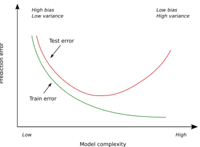
Test error Train error Model complexity P redic tio n er ro r Low High High bias Low variance Low bias High variance
Figure 2.3: Test and training error as a function of the model complexity (Hastie et al., 2003) such a way as to minimize the test error, which is the error of new observations (not used to fit the model). Figure 2.3 shows the typical behavior of train and test error as model complexity is changed. The training error tends to decrease whenever we increase the model complexity, overfitting the data. However, with too much fitting the model adapts too closely and will not generalize well. In contrast, if the model is not complex enough, it will underfit and may have large bias.
2.1.4 Regularization
In the previous sections, given some data D, we minimize some kind of error functionED(w). However, as we mentioned before, minimizing the error term alone is often an ill-posed problem: solutions are not unique and sensitive to data variations. Therefore, a regularization term is usually added to enforce some desirable properties on the solution, such us smoothness, sparsity, low-rank, and so on, changing the criterion function to
J(w) =ED(w) | {z } error +ω(w) | {z } reg. . (2.1.14)
Regularization also helps to control the complexity of the problem and avoid overfitting. For instance if we consider the least square estimates, in theory Theorem 2.1 states that they are the
Best Linear Unbiased Estimates (BLUE), where “best” refers to having the lowest variance. Theorem 2.1 (Gauss-Markov (Plackett, 1950)). Given a linear model with noise ∼N(0, σ),
i.e
y=Xw+, (2.1.15)
then the Ordinary Least Squares (OLS) estimates,
b
w= argminnky−Xwk22o, (2.1.16)
Proof. We begin by showing that they are indeed unbiased. Substituting Eq. (2.1.15) into Eq. (2.1.7) we get, b w= (X>X)−1X>y = (X>X)−1X>(Xw+) =w+ (X>X)−1X>.
Finally, we fix the data matrixX and take expectations on both sides, E[w] =b w+E[(X
>
X)−1X>] =w+ (X>X)−1X>E[] =w, (2.1.17) since E[] = 0 and X is constant. Now we are going to prove that they are the ones with the lowest variance. Let Var(y) =σ2, then the variance of the OLS estimates is
Var(w) = Varb (X>X)−1X>y
= ((X>X)−1X>) Var(y)(X>X)−1X>> = Var(y)((X>X)−1X>)(X(X>X)−1) =σ2(X>X)−1.
Suppose thatwe is another linear estimator, e
w=(X>X)−1X>+Dy, (2.1.18) whereD is ap×n non-zero matrix. The expectation ofwe is
E[w] =e E[((X >X)−1X>+D)y] =E[((X>X)−1X>+D)(Xw+)] =E[((X>X)−1X>+D)(Xw)] +E[(X>X)−1X>+D)] = ((X>X)−1X>+D)(Xw) + ((X>X)−1X>+D)E[] = (X>X)−1X>Xw+DXw = (I+DX)w.
From this we conclude thatDX= 0 for this estimator to be unbiased. The variance of we is Var(w) = Vare (X>X)−1X>+Dy) = Var(y)((X>X)−1X>+D)((X>X)−1X>+D)> =σ2((X>X)−1X>+D)(X(X>X)−1+D>) =σ2((X>X)−1+ (X>X)−1X>D>+DX(X>X)−1+DD>) =σ2((X>X)−1+ 2(X>X)−1(DX)>+DD>) =σ2((X>X)−1+DD>) =σ2(X>X)−1+σ2DD> = Var(w) +b σ2DD> ≥Var(w)b ,
since DD> is a positive semidefinite matrix, that is, DD> ≥ 0. Therefore the least squares estimatorswb are the unbiased linear estimators with the lowest variance, concluding the proof.
However, in practice there are many reason why the least square estimates are not a satisfactory solution to the regression problem. One of these reasons was the non-uniqueness of the OLS solution when the number of variables is larger than the number of observations. Another important one is overfitting.
The simplest example of a regularized model is Ridge Regression, that adds a `2-penalty term to the least squares objective function,
b w= argmin n X i=1 yi− X j wjxij 2 +λX j w2j = argminnky−Xwk2 2+λkwk22 o . (2.1.19)
The previous optimization problem is equivalent to (Hastie et al., 2003)
min n X i=1 yi− X j wjxij 2 s.t X j wj2≤t. (2.1.20)
Using similar arguments to the ordinary least squares case, it is easy to show that Ridge Regression has also a closed form solution
b
w= (X>X+λI)−1X>y. (2.1.21) Note that, in contrast to ordinary least squares, now the matrix (X>X+λI) is always positive definite ifλ >0 and therefore invertible, resulting in a unique solution for the ridge estimates. Furthermore, the previous models favors smaller coefficients and therefore it is less prone to overfitting.
2.2
Convex optimization
We will start these section by defining some basic concepts about convexity in the Euclidean space, although with some more careful work they can be extended to Hilbert spaces. Rn andE are used interchangeably throughout this section to denote the Euclidean space.
Definition 2.1. An Euclidean space Eis a finite-dimensional real vector space with an inner product and its induced norm.
Definition 2.2 (Convex set). A setC ⊆Eis a convex set if for allt∈(0,1) the following holds
tx+ (1−t)y∈C, ∀x, y∈C.
Intuitively, the previous definition means that all the points of the segment joining x and
y must be inside the setC, and this has to be true for any two points in C. For instance an hyperplane H ={x∈Rn : w>x−β = 0} or a ball B ={x ∈
Rn: |x−x0| ≤β} are examples of convex sets. However, the sphereS ={x∈Rn: |x−x
0|=β}provides an example of a set that is not convex (β >0). Figure 2.4 (left) shows another example of an arbitrary convex set. On the other hand, Fig. 2.4 (right) is an example of a non-convex set. It is easy to see that any intersection of two convex sets is also convex. Given I convex setsSi, the finite sum is a new set
S formed by taking all the termsP
si, where si ∈Si, i= 1, . . . , I. Finite sums of convex sets are also convex. We now introduce the concept of effective domain and convex function.
Figure 2.4: Example of convex set (left) and non-covex set (right) [Wikipedia, “Convex set”] Definition 2.3 (Effective domain). The effective domain of f is the set
dom(f) ={x∈E:f(x)<+∞}.
If dom(f) is not empty, the function f is called proper.
Definition 2.4((Strictly) convex function). A functionf :E→R∪ {+∞}is a convex function if dom(f) is a convex set and, for everyx, y∈Eand any t∈[0,1],
f(tx+ (1−t)y)≤tf(x) + (1−t)f(y).
The same function is said to be strictly convex if for everyx, y∈E,x6=y and any t∈(0,1)
f(tx+ (1−t)y)< tf(x) + (1−t)f(y).
The previous definition does not take into account functions that take the value−∞, although it can be expanded to do so (Balder, 2008).
Most machine learning problems are defined as convex optimization problems. The basic definition of an optimization problem has the form:
Definition 2.5 (Primal optimization problem). Given functions f, gi, i = 1, . . . , k, and hi,
i= 1, . . . , m, defined over a domain Ω⊆Rn, the primal problem solves
min f(w), w∈Ω,
s.t gi(w)≤0, i= 1, . . . , k,
hi(w) = 0, i= 1, . . . , m,
wheref(w) is known asobjective function,gi(w) are the inequality constraints andhi(w) are the equality constraints. From now on we are going to write g(w) ≤0 to indicate gi(w) ≤0,
i= 1, . . . , k, and the same withh(w).
Definition 2.5 is general, since maximization problems can be transformed into minimization ones simply by flipping the sign of the objective functionf(w). In the same way, every constraint can be re-written in one of the previous forms. For instance, if we have the constrainP
w< t, we can always write it as P
w−t <0.
The domain region where the objective function is defined and all the constraints are satisfied is known as thefeasible region
Definition 2.6. An optimization problem where the objective function and all the constraints are linear is a linear problem. If the objective function is convex quadratic and the constraints are linear is a quadratic problem.
One of the most well studied problems in optimization is the convex quadratic where the objective function is convex and quadratic and the constraints are linear. The solution of a convex optimization problems is a point w∗ ∈ Rn such that there is no other point w ∈
Rn for which f(w)< f(w∗). This means that any local minimizer w∗ is also a global minimizer. However, note that the minimum does not have to be unique and there can be many points with the same valuef(w∗) of the objective function. Thus, the solution may be a set instead of a single point. If the objective function is strictly convex then it follows from the definition the minimum is indeed unique.
2.2.1 Duality
Lagrange duality is a very important concept in optimization. Given an optimization problem of the form (2.5), it provides us with an equivalent optimization problem that often has comple-mentary properties. Thus, we can choose to indistinctly solve one or the other depending on the situation. We are going to define first the generalized Lagrangian:
Definition 2.7 (Lagrangian function). Given the optimization problem (2.5), we define the generalized Lagrangian function as
L(w,α,β) =f(w) + k X i=1 αigi(w) + m X i=1 βihi(w) =f(w) +α>g(w) +β>h(w).
We can now define the Lagrangian dual problem
Definition 2.8 (Dual optimization problem). The Lagrangian dual problem of the primal problem of Definition 2.5 is the following problem:
max Θ(α,β) s.t α≥0 where Θ(α,β) = infwL(w,α,β)
One of the fundamental relationships between the primal and the dual problem is given by the weak duality theorem, presented next.
Theorem 2.2. (Weak duality theorem) Let w∈Ωbe a feasible solution of the primal problem (2.5) and(α,β) a feasible solution of the dual problem (2.8). Then f(w)≥Θ(α,β).
Proof. From the definition of Θ(α,β) for w∈Ω we have inf
u L(u,α,β)≤L(w,α,β) =f(w) +α
>g(w) +β>h(w)≤f(w). (2.2.2) The last inequality holds since the feasibility of wimplies that
g(w)≤0 and h(w) = 0 (2.2.3)
while the feasibility of α implies
Therefore from Eqs. (2.2.3) and (2.2.4)
β>h(w) = 0 and α>g(w)≤0.
The difference between the values of the primal and dual problems is known as duality gap. The strong duality theorem characterizes what kinds of optimization problems are guaranteed to have a duality gap equal to 0. This means that the dual and the primal problems have the same value. The proof of the strong duality theorem can be found in Ben-Tal and Nemirovski (2001). Theorem 2.3. (Strong duality theorem) Given an optimization problem like the one in
Defini-tion 2.5, where the gi and hi are affine functions, that is
a(w) =Aw−b, (2.2.5)
for some matrixA and vector b, the duality gap is0.
The last theorem of this section characterizes the optimum solution of a general optimization problem (Cristianini, 2000).
Theorem 2.4. (Khun-Tucker) Given an optimization problem in the convex domain Ω⊆Rn min f(w), w∈Ω,
s.t gi(w)≤0, i= 1, . . . , k,
hi(w) = 0, i= 1, . . . , m,
with convex f, affine gi,hi, the necessary and sufficient conditions for a normal pointw∗ to be
an optimum are the existence of α∗ and β∗ such that
∂L(w∗,α∗,β∗) ∂w = 0, ∂L(w∗,α∗,β∗) ∂β = 0, α∗igi(w∗) = 0, i= 1, . . . , k, gi(w∗)≤0, i= 1, . . . , k, α∗i ≥0, i= 1, . . . , k. 2.2.2 Subgradients
We begin this section by briefly reviewing some important definition that will be used in the subsequent chapters.
Definition 2.9(Subdifferential). The subdifferential of a proper convex function is the set-valued map∂f :E→2E, defined as
∂f(x) ={ξ∈E:f(x) +ξ>(y−x)≤f(y), ∀y∈E}
Figure 2.5: A convex function (blue) and “subtangent” lines at x0 (red) [Wikipedia “Subdiffer-ential”]
Let x ∈ E. Then f is subdifferentiable at x if ∂f(x) 6= ∅. The elements of ∂f(x) are the subgradients off atx. Observe that this definition is only non-trivial if the function is proper, that is,x∈domf. Otherwise f(x) = +∞ and∂f(x) =∅. Some properties of the subdifferential are:
(i) For anyx∈E, ∂f(x) is either empty or a closed convex set (see Bauschke and Combettes, 2011, Proposition 16.3).
(ii) For anyx∈int(dom(f)),∂f(x) is not empty and bounded (see Balder, 2008, Lemma 2.16). (iii) ∂f(x) ={∇f(x)} if and only iff is differentiable atx∈E(see Balder, 2008, Proposition
2.6).
(iv) A pointx∈Eis a (global) minimizer off if and only if
0∈∂f(x).
This is known as the Fermat’s rule in convex optimization, and it will be proven later in this chapter.
Let us define first the concept of convex hull, which will be important in what follows. There is also a generalization, the reduced convex hull, where the coefficients are upper-bounded by
µ≤1.
Definition 2.10 (µ-Reduced Convex hull). The µ-reduced convex hull of a set X ={xi}n1 of points in ad-dimensional Euclidean space is the set of all convex combinations of points in X or, more formally, convµ(X) = ( n X i=1 αixi 0≤αi≤µ, ∀i and n X i=1 αi= 1 ) , (2.2.6)
where µ = 1 for the standard convex hull and 1n ≤ µ < 1 for the reduced convex hull. For simplicity we will get rid of the subscript when referring to standard convex hulls. It is easily seen that conv(X) is also the smallest convex set that contains X. This is illustrated in Fig. 2.6.
We will also need some technical results regarding subgradients.
Proposition 2.1 (Maximum of subdifferentiable functions, Boyd and Vandenberghe, 2008).
Suppose f is the pointwise maximum of convex functions f1, . . . , fm, i.e.,
f(x) = max i fi(x),
where the functions fi are subdifferentiable. Then, the subdifferential of f(x) is the convex hull
of the union of subdifferentials of the “active” functions at x, i.e., conv (∪{∂fi(x)|fi(x) =f(x)}).
Proof. Let kbe any index for which fk(x) =f(x) and letg∈∂fk(x). Then, by the definition of subdifferential (Definition 2.9 ) we have,
f(z)≥fk(z)≥fk(x) +g>(z−x) =f(x) +g>(z−x),
andg ∈∂f(x). Thus, to find a subgradient of the maximum of functions, we can choose one of the functions that achieves the maximum at the point, and choose any subgradient of that function at the point. The subdifferential is the set of all such subgradients. Doing that for every pointi= 1, . . . , mwe get that the subdifferential of f is the convex hull of all subdifferentials constructed this way,
conv (∪{∂fi(x)|fi(x) =f(x)}).
Example. The`1-norm
f(x) =kxk1 =|x1|+· · ·+|xn|
is a non-differentiable convex function. Note that it can be expressed as the maximum of 2n linear functions (Boyd and Vandenberghe, 2008):
kxk1 = maxns>x
si∈ {−1, 1} o
.
Therefore we can apply Proposition 2.1 to find the subdifferential. First we have to identify an active functions>x, that is, find ans∈ {−1,1}n such thats>x=kxk1. Since the`1-norm is the sum of the absolute values of the components ofxi, we can take si = +1 ifxi>0 andsi=−1 if
xi <0. Ifxi= 0, more than one function is active and both −1 and 1 work. Thus we can take
si = +1 ifxi>0, −1 ifxi<0, −1 or 1 ifxi= 0.
and apply Proposition 2.1. The subdifferential is the convex hull of all the subgradients that can be generated this way (Boyd and Vandenberghe, 2008):
∂f(x) =ns ksk∞≤1, s >x=kxk 1 o . (2.2.7)
Global minimizers of unconstrained convex optimization problems are characterized by Fermat’s theorem. We need first the definition of proximal mapping:
Definition 2.11 (Proximal mapping). Letf be a lower semicontinuous, proper convex function. Then, te proximal mapping is the operator,
proxf = (I+∂f)−1.
Note also that x= proxf(z) ⇔ z−x∈∂f(x) ⇔ 0∈x−z+∂f(x).
Alternatively, the proximal mapping can be defined also as an optimization problem: Definition 2.12 (Proximal mapping). Letf be a lower semicontinous, proper convex function. For every z∈Rn, the proximal mapping of f is defined as
proxf(z) = argmin y∈R f(y) +1 2||z−y|| 2.
An important example of proximal operator, which will use later in Chapter 3, is the proximal of the `1-norm, f(x) =λ||x||1 =Pni=1|xi|,
[proxf(x)]i = sign(xi) max(0,|xi| −λ). (2.2.8)
This is known as the soft-thresholding operator (see Appendix A for a formal derivation). Fermat’s theorem, presented next, characterizes the solutions of unconstrained optimization problems and it is one of the most important result in convex optimization.
Theorem 2.5 (Fermat’s rule). Let f be a proper convex function. Then,
argminf = zer∂f ={x∈E|0∈∂f(x)} (2.2.9)
and x= proxf(x).
In many optimization problems we further decompose the objective function into two functions: the loss function and the regularizer, as we have seen in Section 2.1.4. The minimization problem then becomes
min x∈E
f(x) +g(x). (2.2.10)
Theorem 2.6 (Moreau-Rockafellar). Letf and g be proper convex functions. Then, for every x0 ∈Rn
∂f(x0) +∂g(x0)⊂∂(f+g)(x0).
Moreover, suppose that int(domf∩domg)6=∅. Then for every x0 ∈Rn we also have
Proof. For the first part, letξ1 ∈∂f(x0) and ξ2 ∈∂g(x0). Then, for allx∈Rn
f(x)≥f(x0) +ξ>1(x−x0)
g(x)≥g(x0) +ξ>2(x−x0) Adding the previous inequalities gives
f(x) +g(x)≥f(x0) +g(x0) + (ξ1+ξ2)>(x−x0) and hence (ξ1+ξ2)∈∂(f+g)(x0). For the second part, check Balder (2008).
Using Fermat’s rule and the previous theorem it is easy to see that the optimality condition for problem (2.2.10) is
0∈∂f(x) +∂g(x).
The previous result does not assume that either f or g are differentiable functions. Most of the times in practice we find that one of them it is indeed differentiable, while the other is not. This can be further exploited to simplify the optimality condition. If the function f is differentiable and Lipschitz continuous, the new optimality condition is
0∈ ∇f(x) +∂g(x),
where we have used the third property of the subdifferential. The next theorem and proposition summarize the previous results.
Proposition 2.2. Let f, g be proper convex functions and f differentiable. Then, the following
are equivalent:
(i) x is a solution of the problem (3.3.17).
(ii) 0∈ ∇f(x) +∂g(x).
(iii) x= proxηg(x−η∇f(x)).
Proof. Ifx is a solution of the problem (2.2.10) then, using Fermat’s theorem (Theorem 2.5), 0∈∂(f +g)(x) ⇔ 0∈∂f(x) +∂g(x) ⇔ 0∈ {∇f(x)}+∂g(x) ⇔ −∇f(x)∈∂g(x) ⇔ x−η∇f(x)∈x+η∂g(x) ⇔ x= proxηg(x−η∇f(x)). 2.2.3 Algorithms
Item (iii) of Proposition 2.2 gives the idea of iterating
xk+1 = proxηg(xk−η∇f(xk)), (2.2.11)
starting from an initial pointx0. It is important to note that, on one hand, wheng= 0, (2.2.11) reduces to thegradient descent method.
for minimizing a Lipschitz-differentiable function (Combettes and Pesquet, 2009). On the other hand, whenf = 0, (2.2.11) reduces to theproximal point algorithm
xk+1= proxηg(xk), (2.2.13)
for minimizing a non-differentiable function (Combettes and Pesquet, 2009). The convergence of this algorithm is guaranteed for an appropriate choice of the parameter η. First we need to precisely definesmoothness,
f(z)≤f(x) +∇f(x)>(z−x) +L
2kz−xk 2
2, (2.2.14)
for all x, z∈Rn. The previous definition is equivalent to
k∇f(x)− ∇f(z)k ≤Lkx−zk. (2.2.15) This condition means that the gradient of the function f is Lipschitz continuous with constant
L. We will sometimes refer to a function f satisfying the previous inequality asL-smooth. The following theorem states the convergence of the Proximal Gradient method:
Theorem 2.7 (Convergence of the proximal gradient method). If f has Lipschitz continuous
gradient with constant L, (f +g) admits minimizers and
η∈ 0, 2 L ,
then the proximal-gradient iterations {xk} converge to a minimizer.
Theory and algorithms for the Lasso
3.1
Lasso
The two standard techniques to improve Ordinary Least Squares (OLS) estimates,subset selection (Hastie et al., 2003) andRidge Regression, both have disadvantages (Tibshirani, 1994). Subset selection obtains interpretable models but it can be very variable since it is a discrete process: features are either kept in the model or dropped from it. On the other hand, Ridge Regression is a continuous process, in the sense that all coefficients are shrunk (but not dropped) and hence more robust. However, it is very rare that coefficients become strictly 0 and therefore models are not interpretable.
Lasso (Least Absolute Shrinkage and Selection Operator) is a technique that reduces (shrinks) some coefficients and sets others to 0; therefore it tries to maintain the advantages of both subset selection and Ridge Regression. Let’s assume, without loss of generality, that thexij are normalized to have zero mean and unit variance, that is,P
ixij/n= 0, Pix2ij/n= 1 and the output variablesyi have zero mean. Letwb = (wb1,wb2, . . . ,wbd)
> be the Lasso estimate, defined by
b w= argmin n X i=1 yi− X j wjxij 2 s.t X j |wj| ≤t, (3.1.1)
wheretis a tuning parameter. This parameter controls the amount of shrinking that is applied to the estimates. Letwbj0 be the full OLS estimates andt0=Pj|wb
0
j|. Values of t < t0, will cause shrinking of the coefficients towards 0, and some coefficients may be strictly 0. For instance if
t=t0/2, the effect will be similar to finding the best subset of sizep/2 (Tibshirani, 1994). On the other hand, ift≥t0,wb
0 is also the solution of the Lasso problem.
The motivation for the Lasso came from an interesting proposal of Breiman, the non-negative garotte (Breiman, 1995) min n X i=1 yi− X j cjwb 0 jxij 2 s.t cj ≥0, X cj ≤t. (3.1.2)
The garotte starts with the full OLS estimates,wb0j, and shrinks them using non-negative factors
cj whose sum is bounded. Thewbj(t) =cjwb 0
j are the new predictor coefficients. Astis decreased, more of the{cj} become 0, and the remaining non-zerowbj(t) are shrunk.
Orthonormal case The orthonormal design case is a highly simplified situation (it is never the case in real-world datasets) where Lasso, subset selection, non-negative garrote and Ridge Re-gression solutions can be computed exactly. This can give interesting insight into the comparative behavior of those methods.
Recall that X is then×dmatrix withij-th entry xij and suppose thatX>X=I. Let wb 0 be the ordinary least squares solution (Chapter 1),
b
w0 = (X>X)−1X>y. (3.1.3) In the case of an orthogonal design, Eq. (3.1.3) simplifies to
b
w0 =X>y.
Using Lagrangian theory, it can be seen (Hastie et al., 2003) that the Lasso problem (3.1.1) is equivalent to b w= argminnky−Xwk22+λkwk1o, (3.1.4) where kwk1= d X j=1 |wj|
and λ≥0. We will prove this equivalence later in Chapter 5. Note that the Lasso penalty is convex, but not strictly convex (refer to Chapter 1 for the definitions). Expanding the first term of the previous equation and using the fact that Xis orthonormal, we gety>y−2ytXw+w>w. Sincey>y does not contain any of the variables to minimize and noting thatwb0 =X>y, we can rewrite the problem (3.1.4) as
b w= argminn2wb0w+kwk22+λkwk1 o = argmin X j 2w0jwj+wj2+λ|wj| , (3.1.5)
where (·)+= max(·,0) denotes the positive part.
The objective function is now a sum of objectives, each corresponding to a separate v