From Linear Classifier to Convolutional Neural Network for Hand Pose Recognition

Pawe l Ro´

sciszewski

FROM LINEAR CLASSIFIER

TO CONVOLUTIONAL NEURAL NETWORK

FOR HAND POSE RECOGNITION

Abstract Recently gathered image datasets and the new capabilities of high-performance computing systems have allowed developing new artificial neural network mo-dels and training algorithms. Using the new machine learning momo-dels, computer vision tasks can be accomplished based on the raw values of image pixels instead of specific features. The principle of operation of deep neural networks resem-bles more and more what we believe to be happening in the human visual cortex. In this paper, we build up an understanding of the most-successful recent mo-del (a convolutional neural network) through the investigation of supervised machine learning methods such as K-Nearest Neighbors, linear classifiers, and fully connected neural networks. We provide examples and accuracy results based on our implementation aimed for the problem of hand pose recognition.

Keywords machine learning, deep neural networks, computer vision

Citation Computer Science 18(4) 2017: 341–356

1. Introduction

Computer vision is an important and fast-growing field of computer science that has various real-life applications, including industrial applications, robotics, and intelli-gent systems [17]. The key tasks of computer vision are image acquisition, preproces-sing, feature extraction, object detection, high-level procespreproces-sing, and decision making. In this paper, we focus on one of the high-level processing tasks –image recognition. The problem of image recognition is to classify each image of a given set to a category. For solving this problem, machine learning methods are used. If the only input of the problem is a set of images, we are dealing with unsupervised learning – the possible classes of objects have to be derived in some way from the data. In this paper, we focus on thesupervised learning problem where each image is labeled with a class name so the possible classes are known a priori.

Usually in machine learning, the labeled examples are divided into a training set and a test set. A model is prepared (trained) using examples from the training set, and then the performance of the model is tested using the test set. There are various approaches to measuring the performance of a model, like accuracy, precision, recall, F-score, etc. [13]. The time needed to train the model is also an important factor. In this work, we focus on the accuracy; namely, the percentage of examples from the test set that were classified to the correct classes. We also provide insights to the distribution of errors by analyzing true positives, true negatives, false positives, and false negatives.

A trained model is a function that takes as an input a set of features of a given example (in this case, an image) and outputs the name (or number) of the predicted class. In traditional image recognition, specifically developed features of the images were used as inputs for the machine learning models. Due to recent advances in neural network models and high performance computing, there is a trend to use raw pixel values as features for classification. The aim of this work is to explore the capabilities of this approach through a case study of the hand pose recognition problem.

The remainder of the paper is organized as follows: In Section 2, we describe the state-of-the-art of the hand pose recognition area. In Section 3, we describe the used image database and problem definition for our case study. The chosen machine learning models and their behavior in our setting are discussed in Section 4. The models are compared in terms of accuracy in Section 5, where we summarize the paper and discuss future work.

2. State-of-the-art in hand pose recognition

Among the head, eyes, face, and arms, hands are considered the most-effective inte-raction tool due to their functionality in communication and manipulation, and they are considered an important part of the HCI (Human-computer interaction) or HRI (Human-robot interaction) methods. The applications of hand gesture recognition

systems include interactive displays, robot motion control, sign language recogni-tion, physical rehabilitarecogni-tion, novel interfaces for mobile devices, and in-car computer interfaces.

The most-effective method for capturing hand motion is with electro-mechanical or magnetic sensors [19]. However, there are many ongoing studies that use computer vision for this purpose, because wearable sensors are relatively expensive and require complex setup and calibration; thus, they are not sufficient for casual use.

The problem of vision-based hand gesture recognition is difficult, because there are many degrees of freedom and interdependences between the fingers. Self-occlusions occur, and there are many possible backgrounds and illumination types in real-life scenarios [6]. Additionally, treating hands as input devices requires real-time response and, thus, a fast processing time in the recognition process.

In the case of real-time HCI systems, partial hand pose estimation is usually used. Unlike the “full DOF” approach (where a 3-D hand model with an estimation of all degrees of freedom is considered in the partial estimation), it is assumed that basic features such as the position of the fingertips and finger orientation and position are sufficient for the system’s needs. The process consists of hand localization, gesture classification, feature extraction, and (finally) pose estimation. In this work, we focus on theclassification part of thesingle frame vision-based hand pose estimation

problem.

The hand gesture recognition problem has been studied extensively in the context of recent advancements in depth imaging and availability of the low-cost Microsoft Kinect motion-sensing input device. Thirty-seven papers in this field have been exami-ned in [20], eleven of which considered exactly the gesture classification part, including approaches involving HMM (Hidden Markov Models), KNN (K-nearest neighbors), Artificial Neural Networks, Support Vector Machines (SVM), Finite State Machines, table-based classifiers, and expectation maximization over Gaussian mixture models. Real-time hand gesture recognition has also been used for interaction with vi-deo games. In [4], the classification part has been accomplished using a multi-class SVM. However, unlike in our approach, the features used for classification were not raw pixels but specific features extracted using the SIFT (Scale Invariant Feature Transform) algorithm.

A set of specific features is also used in [2], where key geometrical features of the hand are used to construct a skeletal hand model. Pre-modeled gesture patterns are prepared beforehand. Gesture recognition is performed by comparing the input gestures with these patterns. The values of certain proximity measures between the models decide the predicted gesture class.

The first dataset containing a sufficient amount of gesture training samples for deep learning methods was proposed in 2013 for a multi-modal gesture recognition challenge. A deep convolutional architecture [12] placed first in the 2014 edition of the competition. The proposed neural network is multi-scale in the meaning that it consists of a combination of paths, each of which performs its own classification

in a certain temporal scale. Each of the classifiers is pre-trained on multiple data modalities, including depth and intensity videos for right and left hands.

Multiple spatial scales have also been combined in a 3D convolutional neural network solution for driver hand gesture recognition in [11]. One of the contributions is combining low- and high-resolution sub-networks in the model, which significantly improves the classification accuracy. The authors also contribute spatio-temporal data augmentation that allows to generate more-feasible training examples and help prevent overfitting (learning the training data too well while not generalizing).

A 3D convolutional neural network was used for large scale user-independent continuous gesture recognition in [3]. The convolutions were performed in three di-mensions (with time as one of the didi-mensions), which allowed for taking into account both the appearance and motion of the images. In [5], a 3D convolutional neural net-work was also used; however, all of the dimensions were spatial dimensions of a depth image this time. The approach allows us to convert a depth map to a 3D volumetric representation of a hand pose.

It is difficult to compare the accuracies of particular approaches, because they are often used for different applications in different setups. In this paper, instead of proposing a new method and comparing it to the existing ones, we provide an overview of the recent advancements in the field of image recognition based on a case study concerning the hand pose recognition problem.

3. Problem definition for our case study

The dataset chosen for this paper is the Cambridge Hand Gesture dataset1. The authors of the dataset [9] proposed a method of classification based on a canonical correlation analysis of tensors. Examples in the machine learning problem were short videos, each consisting of around 60 frames (each with a hand gesture). The gestures were divided into nine classes (three hand shapes ×three movements) from various persons under five different illumination settings.

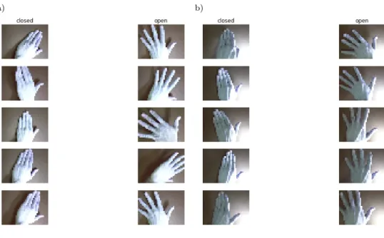
In this work, we focused on single frames rather than videos. We extracted frames with two classes of hand shapes (closed and open) from the datasets with two illumi-nation types. This gave us a training set of 6069 (2887 closed, 3182 open) examples and a test set of 5894 (2991 closed, 2903 open) examples under different illumination. Figures 1a and 1b show randomly chosen examples from each class for the training set and test set, respectively.

Usually before training a model in machine learning problems, the data is pre-processed. An important part of the preprocessing is data normalization. The aim of this step is to ensure that the ranges of values of the training examples for all of their features are more or less similar. This is done because of the training process, which in fact means the optimization of a loss function with respect to the weights.

1

The idea behind normalization is to allow each feature to contribute approximately proportionally to the change of the appropriate weights, which can reduce the time to find the optimal model.

a) b)

Figure 1. Random examples from training and test sets: a) training set; b) test set.

In many approaches to image recognition, also in the one chosen in this paper, features of an image are the raw values of its pixels, naturally falling into a certain unified range. Because of this, we decided to only subtract the mean of all training examples from each example of the training set in the data preprocessing phase. The mean image is shown in Figure 2 (which can resemble a kind of generic palm shape).

4. Chosen classification methods

In this section, we describe how the problem defined in Section 3 can be solved using chosen classification methods such as the K-Nearest Neighbors (Section 4.1), linear classifier (Section 4.2), fully connected neural network (Section 4.3), neu-ral network with one convolutional layer (Section 4.4), and deep convolutional neuneu-ral network (Section 4.5).

4.1. K-Nearest Neighbors

The KNN (K-Nearest Neighbors) algorithm is a particular kind of learning algorithm that requires practically no training. The only operation performed in order to prepare the model is storing all of the training examples. The training examples are then used upon request to classify a new example. Distances from the new example to all training examples are computed according to a certain distance metric. Then, the k

nearest training examples ”vote” for the anticipated class of the new example, each example ”voting” for its own class. The name of the algorithm refers to parameterk, which is a hyperparameter of the algorithm.

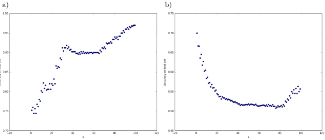
Figure 3 illustrates the accuracies of the KNN algorithm depending on the k

parameter. In the case of evaluating the model on the same examples that were used as the training set, the accuracy roughly increases from around 75% to around 97%, with an increase of k from 1 to 100. The more nearest neighbors that take part in the “vote,” the better the accuracy.

a) b)

Figure 3. Accuracies of KNN algorithm for various values ofk: a) training set; b) test set.

In the case of test set examples, though, the best accuracy is around 70%. The accuracy roughly decreases with thekincreasing from 1 to 80. The more the neighbors “vote,” the greater the chance they make a wrong decision. For higher values of k, the accuracies start getting better (still not exceeding 70%).

The conclusion is that, for examples from a set with a different illumination set-ting, the KNN algorithm performs much worse. It vastly depends on the method of calculating distances between the images that contribute to the decision. In this case, the euclidean (L2) distance was used, so the square root of the sum of squared differences between the corresponding pixels. This is a basic distance, and the met-hods based on it require that the classified object is always in the same position and rotation in the picture. As seen in our case study, this method is also sensitive to changes in illumination.

Although the KNN method can use various approaches to computing the distance between two objects (in this case, images), it still has a supreme flaw related to its training. It requires the storage of all training examples within the model (which, in practice, makes it impossible to use the method in applications employing a large amount of data). Additionally, computing distances between a new example and all of the training examples is too time-consuming in contemporary settings.

4.2. Linear classifier

The linear classifier approach assigns a weight to each feature of the training examples, producing a vector of weights W (in our case, the features are pixels, so W can be treated as a two-dimensional matrix of weights of the same size as the image). For each training example, a score is computed as the sum of the products of the pixel values and the corresponding weights. The scores can be interpreted as weighted averages of the pixels. Usually, there is one weight vectorW per each possible class, and the class with the highest score is chosen as the anticipated class of an image.

In the case of the training set where the correct classes of the training examples are given, a loss function defined for the scores and correct classes allows us to train the model using the back-propagation method [15]. Within this paper, we have im-plemented two loss functions along with the appropriate gradient computations for the back-propagation algorithm. The first-used function is the multi-class version of the hinge loss function (also known as the SVM loss function). The second function is the SoftMax loss function.

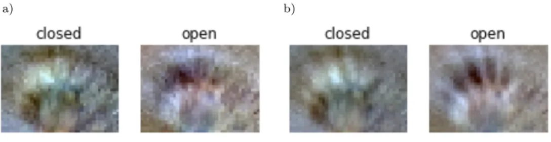
We have trained both versions of the linear classifier using the SGD (Stochastic Gradient Descent) optimization method, obtaining a test set accuracy of around 49% in both cases. We visualized the weights of the trained classifiers in order to conclude the possible reasons for these poor results. What the linear classifier is trying to do is to prepare generic templates of the possible classes (in our case, these would be templates of closed and open palms). The images in Figure 4 present visualizations of trained weight vectorsW for SVM in Figure 4a and SoftMax in Figure 4b. These four templates can be interpreted as kinds of averages of the images from the appropriate classes. Due to the differences between the loss functions, the SVM templates look sharper and the SoftMax templates softer (yet still fairly similar).

As the visualized weights look like traces of waving palms, we can guess that the poor performance of the classification algorithm stems from the rotation of the

training examples. The linear classifier performs better if the objects are equally located and rotated across the training examples. Still, this classification method should be treated as an example that provides intuition of how the more-advanced methods work. It also gives us a good opportunity to practice the implementation of the back-propagation-based training methods.

a) b)

Figure 4. Linear classifier templates: a) SVM template; b) SoftMax template.

4.3. Fully connected neural net

One limitation of the linear classifier described in Section 4.2 is that it can use only one template per category. An apparent idea for improving this situation would be to allow the model to use more of such templates and derive a decision from them.

One way to implement this idea would be a two-layer fully connected neural net (which has been implemented within this work). The two-layer neural network consists of a hidden layer and output layer. Each neuron in the hidden layer can be treated as a single linear classifier, with a separate vectorW.

Before training with the back-propagation algorithm, all of the weights are initia-lized in a stochastic way. Thanks to this, each neuron learns to distinguish a different template during the training. The output layer acts like a perceptron that makes the decision based on the scores of the hidden layer neurons.

There are numerous approaches to connecting neurons from the consecutive layers (called connectivity patterns). In this paper, we used the most-common one where all neurons in one layer are connected to all neurons in the next layer. This type of neural network is called “fully connected” and is used in state-of-the-art computer vision architectures (usually as the last layers of deep network architectures).

It is not difficult to increase the number of hidden layers in a fully connected network (which could improve its performance). However, for the purposes of this paper, we focus on the human-readable interpretation of what a certain model is doing. In order to treat the model as a kind of mixture of linear classifiers, we decided to use one hidden layer with 225 neurons for convenient visualization.

We have trained the two-layer fully connected neural network on the training set using the SGD optimization method. The accuracy of the model on the test set was roughly 67%. The templates learned by the individual neurons are visualized

in Figure 5. It can be seen that the network has trained several different templates falling into two distinct categories (for the two possible classes). Within each class, the templates differ only slightly; however, as the experiment revealed, it is enough to significantly increase the accuracy of the model as compared to the linear classifier. However, we can still see for example that the open hand templates consist of more than five fingers, which suggests that such templates are still sensitive to rotation.

Figure 5. Templates learned by two-layer neural net.

4.4. Neural network with one convolutional layer

The idea of Convolutional Neural Networks (CNN) is surprisingly connected with the findings of 1959 work [7] investigating the visual cortex of a cat. The results of the work revealed that certain neurons in the visual cortex respond with electrical impulses when the cat sees a certain type of shape.

The idea about the principles of operation of the visual cortex is that it is able to understand high-level abstractions by hierarchically combining information about huge numbers of simple shapes and colors. This approach was adopted in computer science decades ago; however, it started to bring satisfactory results around 2012 thanks to the development of new computing architectures.

Instead of class templates for the whole image, a CNN consists of multiple filters. These filters are used as kernels for the convolution operation that is performed for each filter for each possible position in the image, giving multiple scores as inputs for the following layers of the network. It should be noted that the contemporary CNN architectures consist of multiple convolution layers. In such cases, only the first layer has an image as an input, while the inputs for the following layers are outputs of the previous. For the purposes of this paper, we implemented a CNN with one convolutional layer with 21x21 pixel filters, which allowed the visualization of the trained filters in an convenient way.

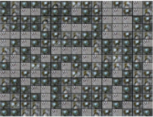
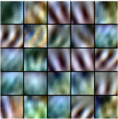
We decided to use the SGD optimization algorithm to train a network with 25 such filters and a fully connected layer with 100 neurons in the hidden layer. Based on numerous experiments, we realized that this optimization method does not suit the CNN model well, giving poor results and random-looking filters. We decided to use the Adam method for stochastic optimization [10], which brought more-satisfactory results. We managed to train a CNN achieving an accuracy of above 85% on the test set. The filters of this network are visualized in Figure 6.

Figure 6. Filters learned by convolutional neural network.

Some of the filters look like groups of fingers in various rotations, which might be the reason for the improvement in accuracy in the CNN model. Another

inter-pretation of these filters is that they resemble Gabor filter [14] for edge detection. Although understanding how a CNN model works is an ongoing study, the model has recently become the default choice for solving computer vision problems. Also in our case study, employing a basic CNN model significantly improved the classification accuracy.

4.5. Deep convolutional neural network

Deep neural networks have recently turned out to be the most-powerful model for many artificial intelligence areas, including computer vision, automatic speech recog-nition, and natural language understanding. The term ”deep” refers to the fact that they are constructed from many layers of neurons, which gives them an outstanding capacity to learn complicated mappings. Image recognition is one of the key areas where deep neural networks have recently enabled the greatest developments. For the case study presented in this paper, we tried training a two-layer convolutional network, but we couldn’t achieve an accuracy better than the 85% that was reported in the case of one convolutional layer described in Section 4.4. One possible reason could be that the training set was too small and data augmentation methods were needed.

Training deep neural networks is a non-trivial task that requires vast amounts of training data. Multiple issues have to be taken into account in the training process that are outside the scope of this paper, including proper weight initialization, pre-venting overfitting through regularization or dropout [18], and the vanishing gradient problem. Additionally, there are multiple parameters of the training process called hyperparameters, whose optimal value can often be determined only through trial and error. These parameters include learning rate, mini-batch size, sizes of hidden layers, weight decays, choosing appropriate nonlinear functions, and more. Advanced methods for searching the hyperparameter space require executing multiple runs of the training process, which requires vast amounts of computational time of the most-efficient high-performance computing hardware. All of these factors make training deep neural networks a hard task.

Fortunately, there is another interesting and useful property of deep neural net-works. Intuitions indicate that, in a properly trained neural network, the consecutive layers learn to distinguish increasingly higher-level features of the training example. For example, the first layer of a deep convolutional neural network learns to dis-tinguish edges, the next ones disdis-tinguishes more and more complicated shapes, and finally the last layer can determine the essential class of a picture. This property is very useful because it allows us to take advantage of thetransfer learningmechanism. In this approach, a previously trained deep neural network can be used as a fea-ture extractor for classification. The activation values (called bottlenecks) of a chosen network layer are computed for each training example. Then, a new classification layer is trained on a given dataset using the values of these bottlenecks as inputs. This way, a new classifier utilizing the great capacity of a deep neural network can be trained

relatively easily. Although the accuracy of such a classifier is usually lower than that of a fully and properly trained model, the approach is sufficiently effective for many applications, requiring only a fraction of the computing time.

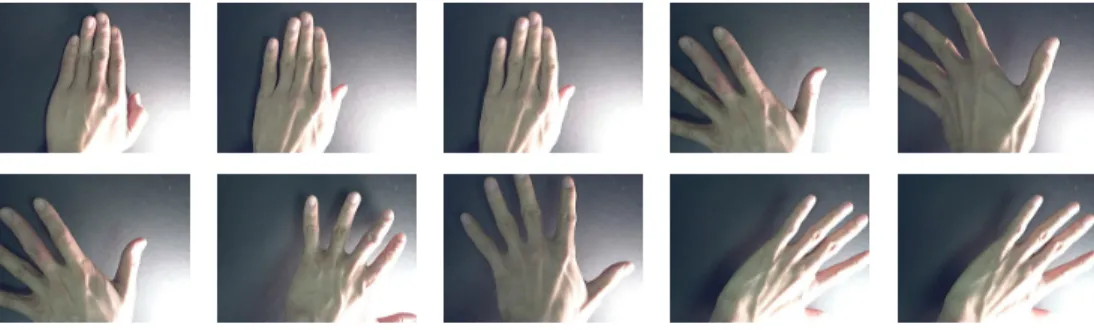
We decided to use the transfer learning method for our hand pose recogni-tion case study. For this purpose, we employed the Inceprecogni-tion-v3 [21] model trained on ImageNet [16], a large-scale hierarchical image database containing more than 14 million human-annotated images. We used the TensorFlow [1] framework to train a SoftMax layer on top of thepool 3 layer of the Inveption-v3 model. We performed 1000 steps of the final layer training on the set used in our case study with a learning rate equal to 0.1. The test-set accuracy of the model turned out to be overwhelming; name-ly, 99.8%. This means that, from 5894 examples in the test set, only 10 examples were incorrectly classified. We present all of the misclassified examples in Figure 7.

Figure 7. Examples incorrectly classified by deep convolutional neural network.

The first three examples are closed palms classified as open ones. In the case of the second and third examples that come from one sequence, the little finger stands away from the rest (which could have mislead the classifier). The remaining open palm examples that were classified as closed were probably difficult to classify due to light reflexes, shadows, and occlusions.

It should be noted that the output of the final SoftMax layer of the model is a vector of the probability values for the two considered classes. Depending on the image recognition application, different methods are used to decide how to use this classification information. The method that achieved the 99.8% precision always chose the class with a higher probability. However, in an end-user application, the probability levels could be utilized in another way that takes classifier certainty into account. Classifications with a class probability below a certain threshold could be repeated on the newly acquired images, which could increase the effective accuracy of the system. In our case study, the average probability of the right class across the whole test set was 0.987, while the average probability of the chosen class in the case of the misclassified examples was 0.745. A threshold of 0.8 confidence would achieve 100% accuracy, introducing the need to repeat the classification for only 68 examples.

5. Summary and future work

In this paper, we discussed the chosen computer vision models on the example of a hand pose recognition case study. We implemented and discussed K-nearest neighbors, linear, fully connected neural network, and convolutional neural network classifiers. The accuracies of the prepared models and numbers of correctly classified examples (OO – open classified as open, CC – closed classified as closed) and incor-rectly classified examples (OC – open classified as closed, CO – closed classified as open) in our setting based on the Cambridge Hand Gesture Dataset are summarized in Table 1.

Table 1

Comparison of implemented methods.

Model OO CC OC CO Accuracy

KNN 1690 2463 1213 528 70%

Linear SoftMax 2839 46 64 2945 49% Linear SVM 2498 389 405 2602 49% Fully connected 2024 1943 879 1048 67% Convolutional one layer 2036 2951 867 40 85% Deep convolutional 2896 2988 7 3 99.8%

Although the compared models are far from being the most-sophisticated and most-effective of their type, the comparison shows that convolutional neural networks are the model that is most capable of reasoning from raw pixels as features of an image instead of complex, hand crafted features. Utilizing a deep convolutional neural network architecture allowed us to achieve a precision of 99.8% on the test set, which would be adequate for many practical applications.

A crucial requirement for the proper training of deep neural architectures is the availability of huge, well-constructed datasets with challenging examples in different surroundings and possible occlusions. Often, datasets prepared for challenge competi-tions are a basis for significant improvements in the field. For example, the VIVA data-set containing 885 intensity and depth video sequences of gestures performed by 8 per-sons inside a vehicle allowed for the development of a deep neural model capable of classifying 19 different dynamic hand gestures with a classification rate of 77.5% [11]. Applying CNNs to a more-difficult definition of the classification problem based on the Cambridge Hand Gesture Dataset, such as the original one [9], should be con-sidered as future work. Particularly, it should be investigated if taking the temporal dimension of the gesture example into account could have a positive influence on mo-del accuracy, especially since previous work in this field [8] states that it does not increase accuracy much as compared to a single-frame-based one.

Acknowledgements

This paper is a result of a project for the courses “Vision in industrial applications and robotics” and “Intelligent systems for industry and environment” under the direction of Prof. Fabio Scotti and Prof. Vincenzo Piuri of the Department of Computer Science, University of Milan. The author would like to sincerely thank Prof. Scotti for his guidance and giving a free hand in choosing research directions. Implementations of the KNN, linear, fully connected and one-convolutional-layer classifiers are based on the assignments of the “CS231n: Convolutional Neural Networks for Visual Reco-gnition” by Stanford University. The image-retraining example of the TensorFlow project has been used for the retraining of the deep convolutional neural network.

References

[1] Abadi M., Agarwal A., Barham P., Brevdo E., Chen Z., Citro C., Corrado G.S., Davis A., Dean J., Devin M., others: TensorFlow: Large-Scale Machine Learning on Heterogeneous Distributed Systems. In: arXiv preprint arXiv:1603.04467, 2016.http://arxiv.org/abs/1603.04467.

[2] Bhuyan M.K., Neog D.R., Kar M.K.: Hand pose recognition using geometric fea-tures. In:Communications (NCC), 2011 National Conference on, pp. 1–5. IEEE, 2011. http://ieeexplore.ieee.org/xpls/abs_all.jsp?arnumber=5734786. [3] Camgoz N.C., Hadfield S., Koller O., Bowden R.: Using convolutional 3d neural

networks for user-independent continuous gesture recognition. In: Pattern Recog-nition (ICPR), 2016 23rd International Conference on, pp. 49–54. IEEE, 2016. http://ieeexplore.ieee.org/abstract/document/7899606/.

[4] Dardas N.H., Georganas N.D.: Real-Time Hand Gesture Detection and Recogni-tion Using Bag-of-Features and Support Vector Machine Techniques,IEEE Tran-sactions on Instrumentation and Measurement, vol. 60(11), pp. 3592–3607, 2011. http://dx.doi.org/10.1109/TIM.2011.2161140.

[5] Deng X., Yang S., Zhang Y., Tan P., Chang L., Wang H.: Hand3D: Hand Pose Estimation using 3D Neural Network. In:arXiv preprint arXiv:1704.02224, 2017. https://arxiv.org/abs/1704.02224.

[6] Erol A., Bebis G., Nicolescu M., Boyle R.D., Twombly X.: Vision-based hand pose estimation: A review, Computer Vision and Image Understanding, vol. 108(1–2), pp. 52–73, 2007.http://dx.doi.org/10.1016/j.cviu.2006.10. 012.

[7] Hubel D.H., Wiesel T.N.: Receptive fields of single neurones in the cat’s striate cortex,The Journal of Physiology, vol. 148(3), pp. 574–591, 1959.

[8] Karpathy A., Toderici G., Shetty S., Leung T., Sukthankar R., Fei-Fei L.: Large-scale video classification with convolutional neural networks. In: Procee-dings of the IEEE conference on Computer Vision and Pattern Recognition, pp. 1725–1732. 2014. http://www.cv-foundation.org/openaccess/content_ cvpr_2014/html/Karpathy_Large-scale_Video_Classification_2014_ CVPR_paper.html.

[9] Kim T.K., Wong S.F., Cipolla R.: Tensor canonical correlation analysis for action classification. In: Computer Vision and Pattern Recognition, 2007. CVPR’07. IEEE Conference on, pp. 1–8. IEEE, 2007. http://ieeexplore.ieee.org/ xpls/abs_all.jsp?arnumber=4270162.

[10] Kingma D., Ba J.: Adam: A method for stochastic optimization. In: arXiv preprint arXiv:1412.6980, 2014.http://arxiv.org/abs/1412.6980.

[11] Molchanov P., Gupta S., Kim K., Kautz J.: Hand Gesture Recognition with 3D Convolutional Neural Networks. In: Proceedings of the IEEE Conference on Computer Vision and Pattern Recognition Workshops, pp. 1–7. 2015.http: //www.cv-foundation.org/openaccess/content_cvpr_workshops_2015/ W15/html/Molchanov_Hand_Gesture_Recognition_2015_CVPR_paper.html. [12] Neverova N., Wolf C., Taylor G.W., Nebout F.: Multi-scale deep learning for

gesture detection and localization. In: Workshop at the European Conference on Computer Vision, pp. 474–490. Springer, 2014.http://link.springer.com/ chapter/10.1007/978-3-319-16178-5_33.

[13] Powers D.M.: Evaluation: from precision, recall and F-measure to ROC, infor-medness, markedness and correlation,Journal of Machine Learning Technologies, vol. 2(1), pp. 37–63, 2011.https://bioinfopublication.org/viewhtml.php? artid=BIA0001114.

[14] Prasad V.S.N., Domke J.: Gabor filter visualization, Technical report, University of Maryland, 2005.

[15] Rumelhart D.E., Hinton G.E., Williams R.J.: Learning representations by back-propagating errors,Nature, vol. 323(6088), pp. 533–536, 1986.http://dx.doi. org/10.1038/323533a0.

[16] Russakovsky O., Deng J., Su H., Krause J., Satheesh S., Ma S., Huang Z., Karpathy A., Khosla A., Bernstein M., Berg A.C., Fei-Fei L.: ImageNet Large Scale Visual Recognition Challenge, International Journal of Compu-ter Vision, vol. 115(3), pp. 211–252, 2015. http://dx.doi.org/10.1007/ s11263-015-0816-y.

[17] Sankowski D., Nowakowski J. (eds.): Computer vision in robotics and industrial applications. No. 3 in Series in computer vision. World Scientific, Singapore, 2014. [18] Srivastava N., Hinton G., Krizhevsky A., Sutskever I., Salakhutdinov R.: Drop-out: A simple way to prevent neural networks from overfitting,The Journal of Machine Learning Research, vol. 15(1), pp. 1929–1958, 2014. http://dl.acm. org/citation.cfm?id=2670313.

[19] Sturman D., Zeltzer D.: A survey of glove-based input,IEEE Computer Graphics and Applications, vol. 14(1), pp. 30–39, 1994.http://dx.doi.org/10.1109/38. 250916.

[20] Suarez J., Murphy R.R.: Hand gesture recognition with depth images: A review. In: 2012 IEEE RO-MAN: The 21st IEEE International Symposium on Robot and Human Interactive Communication, pp. 411–417. 2012.http://dx.doi.org/10. 1109/ROMAN.2012.6343787.

[21] Szegedy C., Vanhoucke V., Ioffe S., Shlens J., Wojna Z.: Rethinking the inception architecture for computer vision. In: Proceedings of the IEEE Con-ference on Computer Vision and Pattern Recognition, pp. 2818–2826. 2016. http://www.cv-foundation.org/openaccess/content_cvpr_2016/html/ Szegedy_Rethinking_the_Inception_CVPR_2016_paper.html.

Affiliations

Faculty of Electronics, Telecommunications and Informatics, Gda´nsk University of Technology, Gda´nsk, Poland,[email protected]

Received: 12.08.2016

Revised: 04.07.2017