PROGRAMA DE PÓS-GRADUAÇÃO EM COMPUTAÇÃO
VINICIUS MEDEIROS GRACIOLLI
A Novel Classification Method Applied to
Well Log Data Calibrated by
Ontology-based Core Descriptions
Thesis presented in partial fulfillment of the requirements for the degree of Master of Computer Science
Profa. Dra. Mara Abel Advisor
CIP – CATALOGING-IN-PUBLICATION Graciolli, Vinicius Medeiros
A Novel Classification Method Applied to Well Log Data Cal-ibrated by Ontology-based Core Descriptions / Vinicius Medeiros Graciolli. – Porto Alegre: PPGC da UFRGS, 2018.
64 f.: il.
Thesis (Master) – Universidade Federal do Rio Grande do Sul. Programa de Pós-Graduação em Computação, Porto Alegre, BR– RS, 2018. Advisor: Mara Abel.
I. Abel, Mara. II. Título.
UNIVERSIDADE FEDERAL DO RIO GRANDE DO SUL Reitor: Profa. Rui Vicente Oppermann
Pró-Reitora de Coordenação Acadêmica: Profa. Jane Fraga Tutikian
Pró-Reitor de Pós-Graduação: Prof. Celso Giannetti Loureiro Chaves Diretora do Instituto de Informática: Profa. Carla Maria Dal Sasso Freitas
Coordenador do PPGC: Prof. João Luiz Dihl Comba
ACKNOWLEDGMENTS
I would like to thank first and foremost my advisor Mara Abel for all her support prior and during this work. I would also like to thank my colleagues Eduardo, Lucas, Júlia, Renata and Elias who helped me process the data cordially ceded by ANP and Petrobras. This work would also not be possible without the help of Luiz Fernando De Ros who provided support with the geological part of this work.
I would also like to thank Jean-François Rainaud and his wife Marie-Laure for being such gracious hosts and providing me with the opportunity to spend a wonderful time in France.
LIST OF ABBREVIATIONS AND ACRONYMS . . . . 7 LIST OF FIGURES . . . . 8 LIST OF TABLES . . . . 11 ABSTRACT . . . . 12 RESUMO . . . . 13 1 INTRODUCTION . . . . 15
2 STATE OF THE ART . . . . 20
3 PREVIOUS WORK IN THIS PROJECT . . . . 23
3.1 Automatic Bedding Discriminator . . . 23
3.2 Enhancements . . . 25
4 DOMAIN ONTOLOGY OF SEDIMENTARY FACIES . . . . 27
4.1 The StrataledgeR1Ontology . . . . 28
5 WIRELINE LOGS . . . . 30
5.1 The LAS File . . . 30
5.2 Correlation Logs . . . 30 5.2.1 Spontaneous Potential . . . 31 5.2.2 Gamma Ray . . . 31 5.2.3 Caliper . . . 31 5.3 Porosity Logs . . . 31 5.3.1 Sonic . . . 32 5.3.2 Density . . . 32 5.3.3 Neutron . . . 32 5.4 Resistivity . . . 32 5.4.1 Induction . . . 32 5.4.2 Laterolog . . . 33 5.4.3 Microresistivity . . . 33
6 DESCRIPTION OF THE TESTING DATA . . . . 34
6.1 Testing Data Analysis . . . 35 1STRATALEDGE is a trademark of ENDEEPER Co.
7 METHODOLOGY . . . . 46 7.1 Detecting Intervals . . . 46 7.2 Determining Lithology . . . 47 8 RESULTS . . . . 50 9 CONCLUSION . . . . 54 REFERENCES . . . . 56 ANNEX 1 . . . . 58 ANNEX 2 . . . . 62
KNN K-Nearest Neighbor NN Neural Network
BNN Bayesian Neural Network HMM Hidden Markov Model SVM Support Vector Machine LDA Linear Discriminant Analysis CRF Conditional Random Field NB Naïve Bayes
ABD Automatic Bedding Discriminator DT Sonic interval transit time
GR Gamma Ray
NPHI Neutron porosity RHOB Bulk density DRHO Density correction ILD Induction resistivity LAS Log ASCII Standard
LIST OF FIGURES
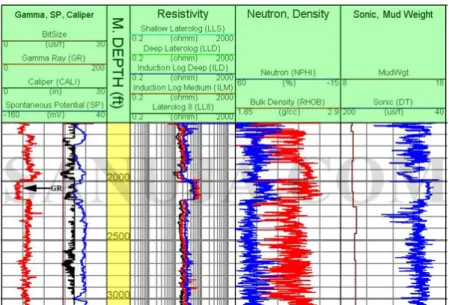
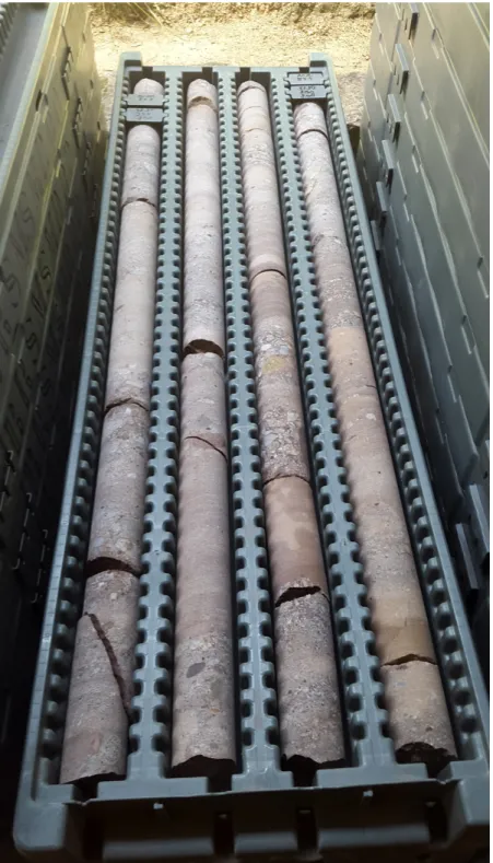
1.1 Example of a well log report. Each line represents a different geo-physical measurement, as outlined in the image header. The verti-cal axis measures the depths at which the measurements were taken. Source (SENANYAKE, 2016. Available at http://sanuja.com/blog/what-is-a-well-log. Accessed Mar 22 2018) . . . 16 1.2 Example of a box containing a sequence of core samples labeled by
depth. . . 17 1.3 Example of a non-standardized core description made with freehand
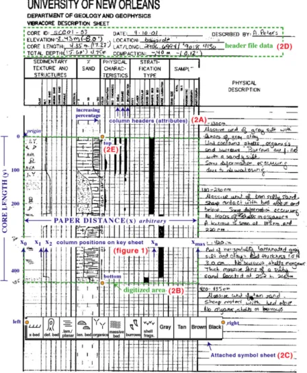
drawings and text. The labels show column attributes (2A), area be-ing digitized (2B - outlined green box), attached symbol menu (2C), header information (such as latitude, longitude, and elevation) (2D - dashed green box), and locations of first four digitized points: top and bottom of core, and left and right side of symbol menu (2E). Columns are recognized by their distance from origin (x-value), and vertical dimension (y) is either core length or depth of core pene-tration relative to a datum. Source: (USGS, 2010. Available at https://pubs.usgs.gov/ds/542/. Accessed Mar 22 2018.) . . . 18 3.1 Result of moving means being used to detect change points in an
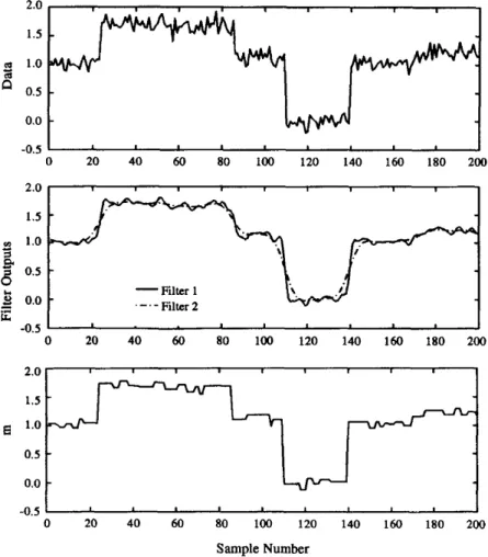
arbitrary dataset. Filter 1 is obtained by applying a small moving window to the original data, Filter 2 by applying a larger one. The final result displayed is obtained by averaging all values between each intersection. Source (MACDOUGALL; NANDI, 1997) . . . 24 3.2 Example showing the integration of break point results. Each vertical
black line represents a log from the same well, where break points were detected at the red markers. The numbers on top of each log corresponds to the weight of that log. The orange sections on the logs represent the depths encompassed by the agreement window ws. If we consider a weight of3to declare breaks, a break will be recorded in the final assessment on the depth corresponding to the mean depth of the three breaks crossed by the green line, as the sum of the three logs with breaks within that depth’s tolerance window is greater or equal than 3. . . 26 4.1 Representation model of sedimentary facies built by a propositional
term and a pictorial icon. The icon resembles the visual aspect of the facies. Source: (ONTOLOGICAL PRIMITIVES FOR VISUAL KNOWLEDGE, 2010) . . . 28
ITIVES FOR VISUAL KNOWLEDGE, 2010) . . . 29 6.1 Box plot of the log values for each of the lithologies present in the
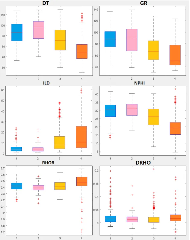
testing data. The logs present in this data are Gamma Ray (GR), Sonic (DT), Density (RHOB, DRHO) and Neutron (NPHI). The litholo-gies are color coded based on the group to which they were assigned. The sand/clay heterolite belongs to group 2 (pink), and contains only one sample. While the other two lithologies in group 2 seem to have contrasting signatures, this is due to the low number of samples on the Sand/silt heterolite not being representative enough to create an accurate model . . . 37 6.2 Box plot of the log values for each of the lithologies present in the
testing data. Notice the contrast in distributions between groups 3 and 4 (sandstone and conglomerates) and the other lithologies. . . 38 6.3 Plot of the samples contained in Well 1. Each square presents a
scat-terplot of two logs, the diagonal shows histograms of the distribution of each of the logs. . . 39 6.4 Plot of the samples contained in Well 2. Each square presents a
scat-terplot of two logs, the diagonal shows histograms of the distribution of each of the logs. . . 40 6.5 Plot of the samples contained in Well 3. Each square presents a
scat-terplot of two logs, the diagonal shows histograms of the distribution of each of the logs. . . 41 6.6 Plot of the samples contained in Well 1 grouped in the way described
in this chapter. Each square presents a scatterplot of two logs, the diagonal shows histograms of the distribution of each of the logs. . . 42 6.7 Plot of the samples contained in Well 2 grouped in the way described
in this chapter. Each square presents a scatterplot of two logs, the diagonal shows histograms of the distribution of each of the logs. . . 43 6.8 Plot of the samples contained in Well 3 grouped in the way described
in this chapter. Each square presents a scatterplot of two logs, the diagonal shows histograms of the distribution of each of the logs. . . 44 6.9 Plot of the samples contained in the first synthetic dataset. Each
square presents a scatterplot of two artificial logs, the diagonal shows histograms of the distribution of each of the logs. . . 45 6.10 Plot of the samples contained in the second synthetic dataset. Each
square presents a scatterplot of two artificial logs, the diagonal shows histograms of the distribution of each of the logs. . . 45 6.11 Plot of the samples contained in the third synthetic dataset. Each
square presents a scatterplot of two artificial logs, the diagonal shows histograms of the distribution of each of the logs. . . 45 7.1 This framework shows an overall view of our method for lithology
detection, the processes involved and what data artifacts are used and generated. . . 46 9.1 Sedimentary Facies and its attributes. . . 61
9.2 Plot of data from Well 1 . . . 62 9.3 Plot of data from Well 2 . . . 63 9.4 Plot of data from Well 3 . . . 64
6.1 This table shows the number of samples for each lithology in the three wells chosen for the test case. . . 35 8.1 Classification accuracy achieved on the synthetic dataset with
dif-ferent variations of the method developed, compared to the method described in (BOSCH; LEDO; QUERALT, 2013a). . . 50 8.2 Classification accuracy achieved on the real dataset with different
variations of the method developed, compared to the method described in (BOSCH; LEDO; QUERALT, 2013a). . . 51 8.3 Classification accuracy in each well using the method developed on a
complete split test with and without the use of the Bayesian prior. . . 51 8.4 Classification accuracy in each well using a KNN classifier, the
num-ber after KNN specifies how many neighbors the classifier takes into account. Using more than 40 neighbors makes little sense consider-ing the number of samples in the trainconsider-ing data. The NN line stands for the classification accuracy of the neural network. . . 52 8.5 Results from the application of the multi-agent system assembled on
ABSTRACT
A method for the automatic detection of lithological types and layer contacts was developed through the combined statistical analysis of a suite of conventional wireline logs, calibrated by the systematic description of cores.
The intent of this project is to allow the integration of rock data into reservoir mod-els. The cores are described with support of an ontology-based nomenclature system that extensively formalizes a large set of attributes of the rocks, including lithology, tex-ture, primary and diagenetic composition and depositional, diagenetic and deformational structures. The descriptions are stored in a relational database along with the records of conventional wireline logs (gamma ray, resistivity, density, neutrons, sonic) of each an-alyzed well. This structure allows defining prototypes of combined log values for each lithology recognized, by calculating the mean and the variance-covariance values mea-sured by each log tool for each of the lithologies described in the cores. The statistical algorithm is able to learn with each addition of described and logged core interval, in order to progressively refine the automatic lithological identification.
The detection of lithological contacts is performed through the smoothing of each of the logs by the application of two moving means with different window sizes. The results of each pair of smoothed logs are compared, and the places where the lines cross define the locations where there are abrupt shifts in the values of each log, therefore potentially indicating a change of lithology. The results from applying this method to each log are then unified in a single assessment of lithological boundaries.
The mean and variance-covariance data derived from the core samples is then used to build an n-dimensional gaussian distribution for each of the lithologies recognized. At this point, Bayesian priors are also calculated for each lithology. These distributions are checked against each of the previously detected lithological intervals by means of a prob-ability density function, evaluating how close the interval is to each lithology prototype and allowing the assignment of a lithological type to each interval.
The developed method was tested in a set of wells in the Sergipe-Alagoas basin and the prediction accuracy achieved during testing is superior to classic pattern recognition methods such as neural networks and KNN classifiers. The method was then combined with neural networks and KNN classifiers into a multi-agent system. The results show significant potential for effective operational application to the construction of geological models for the exploration and development of areas with large volume of conventional wireline log data and representative cored intervals.
Keywords: Core-log integration, geophysical log, core description, lithology interpreta-tion.
Um método para a detecção automática de tipos litológicos e contato entre camadas foi desenvolvido através de uma combinação de análise estatística de um conjunto de perfis geofísicos de poços convencionais, calibrado por descrições sistemáticas de testemunhos. O objetivo deste projeto é permitir a integração de dados de rocha em modelos de reservatório. Os testemunhos são descritos com o suporte de um sistema de nomencla-tura baseado em ontologias que formaliza extensamente uma grande gama de atributos de rocha. As descrições são armazenadas em um banco de dados relacional junto com dados de perfis de poço convencionais de cada poço analisado. Esta estrutura permite definir protótipos de valores de perfil combinados para cada litologia reconhecida através do cálculo de média e dos valores de variância e covariância dos valores medidos por cada ferramenta de perfilagem para cada litologia descrita nos testemunhos. O algoritmo estatístico é capaz de aprender com cada novo testemunho e valor de log adicionado ao banco de dados, refinando progressivamente a identificação litológica.
A detecção de contatos litológicos é realizada através da suavização de cada um dos perfis através da aplicação de duas médias móveis de diferentes tamanhos em cada um dos perfis. Os resultados de cada par de perfis suavizados são comparados, e as posições onde as linhas se cruzam definem profundidades onde ocorrem mudanças bruscas no valor do perfil, indicando uma potencial mudança de litologia. Os resultados da aplicação desse método em cada um dos perfis são então unificados em uma única avaliação de limites litológicos.
Os valores de média e variância-covariância derivados da correlação entre testemu-nhos e perfis são então utilizados na construção de uma distribuição gaussiana n-dimensional para cada uma das litologias reconhecidas. Neste ponto, probabilidades a priori também são calculadas para cada litologia. Estas distribuições são comparadas contra cada um dos intervalos litológicos previamente detectados por meio de uma função densidade de probabilidade, avaliando o quão perto o intervalo está de cada litologia e permitindo a atribuição de um tipo litológico para cada intervalo.
O método desenvolvido foi testado em um grupo de poços da bacia de Sergipe-Alagoas, e a precisão da predição atingida durante os testes mostra-se superior a algorit-mos clássicos de reconhecimento de padrões como redes neurais e classificadores KNN. O método desenvolvido foi então combinado com estes métodos clássicos em um sistema multi-agentes. Os resultados mostram um potencial significante para aplicação operacio-nal efetiva na construção de modelos geológicos para a exploração e desenvolvimento de áreas com grande volume de dados de perfil e intervalos testemunhados.
Palavras-chave:integração perfil-testemunho, perfil geofísico, descrição de testemunho, interpretação litológica.
1
INTRODUCTION
This work details the development of a novel technique for data classification applied to geological data. This classification consists of associating numerical data samples with classes representing specific rock types. The framework developed attempts to emulate the behavior of the geologist commonly assigned to this task by segmenting data prior to the use of a classification algorithm; as opposed to classifying the samples independently, as it is commonly done in applications that attempt to solve this task automatically.
In the process of petroleum exploration and development, massive amounts of data are generated with the goal of locating possible oil reservoirs and determining their viability. This data can span scales ranging from the continental to the microscopic. When a rock formation containing oil reserves is found, this data is used to build 3D reservoir models that can be used to simulate the production potential of the reservoir. The goal of this work is to ultimately enrich these models by providing a tool that can be used to infer additional information from the available data, which can then be added to the model in locations where this information is missing.
The main datasets used to create these models come from seismic imaging and well data. Seismic imaging consists of taking images of the subsurface of the selected lo-cation that are produced using seismic echography; by laying acoustic sensors on the ground at regular intervals and detonating explosive charges these subsurface images can be constructed by measuring the time it takes for the acoustic waves to penetrate the rock formation and be reflected back to the sensors. These sensors can be spread across as several square kilometers, and with these images, which reflect the density and shape of the underlying rock formations.
Well data includes geophysical information and rock samples. This geophysical in-formation is presented as wireline logs, which are numerical measurements taken from tools lowered down the well during or after perforation. These tools can gauge many dif-ferent properties of the rock formation such as resistivity, conductivity, sonic transit time or gamma ray emissions, producing reports such as the one depicted in figure 1.1 that shows a single well with several geophysical measures aligned by depth. With these logs, properties such as porosity, grain size or the presence of fluids can be inferred based on the response of the log. When there are several available wells in the same sedimentary basin, they can be integrated to support the generation of a 3D model of the reservoir.
The recovery of rock samples allows direct access to rocks located many hundreds of meters underground. There are many types of rock samples that can be recovered and analyzed; detritus that leaves the borehole during drilling for instance, can inform the type of rock present in the drilled area within a reasonably precise depth. More detailed samples are also recovered from the well during and after drilling, such as sidewall cores, which are samples taken from wall of the borehole via mechanical or percussion drilling
16
Figure 1.1: Example of a well log report. Each line represents a different geophysical measurement, as outlined in the image header. The vertical axis measures the depths at which the measurements were taken. Source (SENANYAKE, 2016. Available at http://sanuja.com/blog/what-is-a-well-log. Accessed Mar 22 2018)
at specific depths. Objective measurements can also be taken by submitting a rock sample to laboratorial analysis, to calculate attributes such as density, microporosity and perme-ability.
The most valuable sample that can be extracted from the well however, is the core sample, which is a whole cylindrical section of the borehole which is extracted during drilling without being destroyed in the process. Figure 1.2 shows a box containing core samples collected from a well for further description. The recovery of a core sample is an expensive process, since it requires the drilling to stop, and the regular drilling head to be replaced by a special drill with a hollow center to allow for the recovery of the core. For that reason, a borehole spanning several kilometers may only have a couple hundred meters of cores recovered. As the core is retrieved relatively intact, it can offer important information about the structure of the rock formation, as well as allow the analysis of the contacts between each layer of rock. These samples can be analyzed by a geologist which generates a qualitative description of the rock formation based on the perceived characteristics of the rock sample. The qualitative description is a hand-made task that produces reports similar to those presented in Fig XX
This work focuses on the correlating lithology data, which is a qualitative assessment of the rock characteristics recorded in the core descriptions, with readings taken from wireline logs. The goal is to be able to extrapolate these rock characteristics based on the much more common wireline log data, which can span most of the depth of the well. This is a pattern recognition problem, where a series of numerical measurements taken at a specific depth in the borehole are labeled as a lithology, based on the readings taken at depths with previously known lithologies. This work uses a novel approach where prior to being labeled, the samples are grouped based on their context within the borehole; by detecting sudden changes in the log values, likely depths at which a lithological change may occur set the boundaries between these groups. This grouping process is shown to increase the prediction accuracy when used in tandem with the method developed to label the samples analyzed.
18
Figure 1.3: Example of a non-standardized core description made with freehand drawings and text. The labels show column attributes (2A), area being digitized (2B - outlined green box), attached symbol menu (2C), header information (such as latitude, longitude, and elevation) (2D - dashed green box), and locations of first four digitized points: top and bottom of core, and left and right side of symbol menu (2E). Columns are recognized by their distance from origin (x-value), and vertical dimension (y) is either core length or depth of core penetration relative to a datum. Source: (USGS, 2010. Available at https://pubs.usgs.gov/ds/542/. Accessed Mar 22 2018.)
This work relies on three hypotheses. First, that we can increase the classification accuracy on lithology prediction by separating the data in segments corresponding to homogeneous rock sections. Second, that the boundaries between these rock sections should be detectable by a sudden change in log value. And third, that each lithology has a distinct log signature.
The method used for classification is a gaussian classifier based on supervised learn-ing, where the inference process is calibrated by a training set composed of a set of wire-line logs and core descriptions which provide the lithology labels for sampled depths in the wireline logs. The framework developed was trained and tested with real well data from the Sergipe-Alagoas basin, and the classification accuracy was tested against other classic machine learning methods for pattern recognition such as fuzzy classifiers, neural networks and k-nearest neighbors classifiers. The results show that the method developed achieves a classification accuracy comparable to or greater than these other algorithms.
By inferring this lithology data in well scale, this information can later be extrapolated to a larger scale by integrating this information into reservoir models built from seismic imaging in uncored sections, where there is no lithology information.
This work is organized in the following structure. First, the current methods for lithol-ogy identification methods are analyzed and their shortcomings are identified. Then we present a summary my previous work and how it relates to the method developed. Later, the datatypes which are used in this work are introduced and explained. Then, the data used for testing is presented and analyzed. Finally, the framework for lithology interpre-tation developed is presented, tested and compared to other classification methods, from which we draw our final conclusions.
20
2
STATE OF THE ART
Predicting lithology from wireline logs is not a novel idea; much work has been done in this area attempting to predict lithotypes from log values. Where most of these works fall short is when it comes to the testing data. Synthetic datasets are often used, and they can show a vastly different reality from the average borehole. Even when done with real data, samples may be classified not by actual inspection of the rock formation, but by grouping the samples through clustering algorithms.
Neural networks are a popular solution for pattern recognition problems such as this, which boils down to recognizing a pattern of log signatures and assigning a lithology value based on these measurements. Neural networks work as a series of nodes passing along numerical values through weighted connections. By training the network with a set of data containing inputs and expected outputs, these weights are adjusted by means of a backpropagation algorithm until the output of the neural network is in line with the expected output.
Reid (REID; LINSEY; FROSTICK, 1989) describes an approach that he has called theAutomatic Bedding Discriminator, a method to detect boundaries between lithologies based on gamma ray logs. This is done by using moving means to detect sudden changes in the log data, which characterize a change in lithology. The method can then discrimi-nate between rocks with larger or smaller grain sizes based on the deflection of the log at these change points, this is possible due to the gamma ray log used being highly sensitive to grain size. This method forms the basis of the first part of this work, which allows the separation of the logged interval into discrete sections.
Coudert (COUDERT; FRAPPA; ARIAS, 1994) uses gaussian distributions to build prototypes in a similar way to the method developed in this work. However, Coudert’s gaussian distributions are all one-dimensional, as opposed to the multivariate distributions used in this work. Once the prototypes have been calculated by correlating log values and rock samples, they are compared to the prototypes through a probability density function. To increase prediction accuracy, Coudert also uses Bayesian priors and rules based on geological principles to determine lithology on uncertain situations. Due to the use of these rules, Coudert’s method is not as flexible as this work when it comes to adaptation to different rock characteristics or other problems.
Brereton (BRERETON; GALLOIS; WHITTAKER, 2001) uses a clustering method that distributes sampled points in a color space based on the readings of the wireline logs, and then assigns a lithological significance to these points based on the area of the color space that was assigned to them. While it discerns the most contrasting changes in lithol-ogy with reasonable accuracy, it also detects a large number of lithological changes not described in the validation data. While the article claims that these are subtle variations not easily detected by the geologist doing the core description, it also means the results
can only be truly validated against the rock sample themselves, not against descriptions that can not be revisited.
Li (LI; ANDERSON-SPRECHER, 2006) compared a naive Bayes classifier with lin-ear discriminant analysis (LDA) and found both methods to perform adequately on a set of data from three well consisting of gamma-ray (GR), neutron porosity (NPHI), forma-tion density (RHOB), and deep resistivity (LLD) logs and core descripforma-tions from which five distinct facies, which were not entirely based on lithology were identified. The top prediction accuracy of Li’s work reached 81.2% with the linear discriminant analysis ap-proach.
Al-Anazi (AL-ANAZI; GATES, 2010) shows an approach based on a support vector machine (SVM). Support vector machines can generate mapping functions through super-vised learning which allows the samples to be separated by a hyperplane in n-dimensional space. Al-Anazi’s work focuses on predicting permeability, and suffers from the lack of hard rock data, as validation is made through comparisons with known electrofacies.
Gifford (GIFFORD; AGAH, 2010) uses neural networks, along with other learning algorithms such as k-nearest neighbors (KNN) classifiers in a multi-agent system. In this approach, the problem is solved by multiple independent modules, each using a different method. These results are then integrated into a final output, resulting in a higher accuracy than any individual method used. The complete system presented in the article achieves a top accuracy of 84.3%.
The problem with neural network based approaches is that the training is expensive in terms of processing power, requiring a large dataset to avoid overfitting. While it can produce good results, the series of calculations learned and performed by a neural network are often seen and treated as a black box, for peering inside it reveals a series of low level processes that are difficult to be understood by a human reader.
Bosch in (BOSCH; LEDO; QUERALT, 2013b) describes a fuzzy logic based method that was implemented as a MATLAB routine for the task of facies classification. In this method, membership functions are calculated from the training data in order to classify a validation set by measuring the degree of membership of sample to each lithology in a manner similar to the method developed in this work. In Bosch’s work, his method was tested using synthetic data. Since the implementation of Bosch’s work was made public, it has been tested with the data used in this work for the purposes of comparison with the method developed.
Ojha (OJHA; MAITI, 2013) presents a Bayesian Neural Network (BNN) based ap-proach that optimizes the starting weights of his neural network, decreasing the training time needed until the neural network starts to produce reasonable results. The network is then trained using a data set derived from clustering and statistical analysis of wireline log data. In the presence of 10% red noise, the method presented in the article achieves an average accuracy of 67.38%.
Jeong (JEONG et al., 2014) uses a Hidden Markov Model (HMM) and a Conditional Random Field (CRF) based approach to tackle lithology prediction. A HMM can be seen as a sequential version of a naive Bayes (NB) classifier, which learns how to classify data through a joint distribution of the training data. On the other hand, a CRF can be seen as a sequential version of a logistic reversion classifier, which learns from conditional distribution. While Jeong’s work managed up to 82% prediction accuracy, it was tested using synthetic data.
Some limitations are show to be very prevalent in the methods presented in the litera-ture, namely the usage of low quality or synthetic data, and the fact that all these methods
22
treat each data sample individually, ignoring the context in which they are inserted. The method described in this work introduces a new approach where the data is segmented into facies prior to classification. This segmentation is done using a moving-means based al-gorithm derived from Reid’s work, which was adapted to work with multiple logs instead of relying solely on the gamma ray readings. These segments are then labeled by compar-ing the samples contained within against multivariate gaussian distributions derived from correlation between well logs and core descriptions in a training set. This approach has the benefit of increasing classification accuracy by analyzing the data samples within the context of a contiguous body of rock, instead of isolated datapoints.
3
PREVIOUS WORK IN THIS PROJECT
The framework described in this work bases its first step in the research previously presented in (GRACIOLLI, 2014), where wireline logs are used to determine lithological boundaries which can then be correlated to descriptions of core samples in order to correct any possible offsets between the core and log depths resulting from faulty data acquisition. The method developed uses the boundary information obtained from application of that previous work as a way to enhance the accuracy of pattern recognition methods when applied to the task of lithological identification in a novel way which is not explored by the methods currently used in this task.
This segmentation method is based on the work done by Reid (REID; LINSEY; FRO-STICK, 1989) which is briefly mentioned in the previous chapter, but expanded in order to accommodate working with multiple wireline logs, instead of being restricted to the gamma ray log. Reid’s work, as well as the enhancements developed in (GRACIOLLI, 2014) are described in the next section.
3.1
Automatic Bedding Discriminator
Reid’s boundary detection algorithm is dubbed theAutomatic Bedding Discriminator. His method starts from the assumption that a lithological change can be characterized in the log reading by a sudden change in log values. Reid’s work uses exclusively gamma ray logs to build a boundary assessment; which is one of the most common logs taken from a borehole. The Gamma Ray log responds to the organic matter content of the rock and has a high correlation to grain size, which makes it useful to detect intercalated sandstone-shale layers.
The first step in detecting these sudden changes is to deal with signal noise. Log readings can be affected by a wide number of variables such as borehole size or the com-position of the drilling mud used during perforation. Even small scale changes in lithol-ogy that are not detected by the geologist on a core sample or do not characterize a clear change in lithology can be picked up by the logging tools and appear as slight changes in log value.
This noise is dealt with by applying a centered moving mean to the log data. The value of a centered moving mean at the data pointdp with a window of sizen is defined
as the average value of then closest data points to point dp (includingdp). This results
in a loss of data, so care must be taken to not use a window that is too large, which will discard meaningful log features; nor a window that is too small, which won’t effectively filter out variations induced by noise. Reid’s work suggests a window of around 1m for this step, since information is rapidly lost with windows larger than 2m.
24
the aim of deriving a curve that shows the general trend of the log; for this, Reid suggests a window of approximately 10m. By comparing both filtered logs, the points where there are sudden changes in log values can be determined by checking at which positions both logs intersect; in essence, where the log increases or decreases more than it’s general trend. This is done simply by checking at each data point if the status quo of which filtered log is higher than the other is either maintained or inverted, if the previously lower-valued log turns becomes the higher-valued log, that means the logs have intersected. A visual representation of the result of this process can be seen in figure 3.1.
Figure 3.1: Result of moving means being used to detect change points in an arbitrary dataset. Filter 1 is obtained by applying a small moving window to the original data, Filter 2 by applying a larger one. The final result displayed is obtained by averaging all values between each intersection. Source (MACDOUGALL; NANDI, 1997)
Another consideration taken inReid’s Automatic Bedding Discriminator is with sec-tions of the log where there is little change across a long section of measured depths; in these cases the values of both smoothed logs may be very similar, and very small alter-ations in the log value may register as an intersection between the smoother logs. In order to deal with this situation and cull the resulting false positives from the assessment, Reid establishes a threshold of 4 API1 and disregards detected changes in lithology resulting from a change in log value lower than this threshold.
1API is a measurement originated from the petroleum industry, and is the standard unit of measurement
Reid’s method then attempts to classify the facies found in the previous step of his algorithm by analyzing the deflection on the log curve at the points where a bedding contact was detected. By assessing the sign and magnitude of the change in log value, it is possible to estimate the increase or decrease in grain size which can differentiate between shale and sandstone.
3.2
Enhancements
Reid’sAutomatic Bedding Discriminatorresults in an assessment of break points for a single gamma ray log, but the method can be expanded in order to take into account other logs that may also have important lithological significance, such as porosity, density and resistivity logs (OJHA; MAITI, 2013); by applying it to multiple logs and then integrating the results in an unified assessment. Before this can be done, however, some issues must be taken into consideration: first, wireline logs have varying degrees of representativeness for lithological assessment (KRYGOWSKI, 2003); second, the same bedding contact is not likely to be detected at the exact same depth across multiple logs.
The first problem can be solved by assigning a weightwto each log, which is checked against a user defined thresholdtwhen declaring break points: if the sum of the weights of all logs accusing a break at depthdis equal or greater than the thresholdt, we say there is a break at depthd. The ideal weights can be affected by the type of sedimentary terrain. Considering that the field available for validation in this work is mostly composed by sili-ciclastic rocks with minor presence of carbonates, the following guidelines for assigning weights were proposed by the inquired geologists:
• Gamma Ray logs are the most representative for lithological changes, and thus should have the highest weight.
• Density and porosity related logs are also highly representative and thus should have weights close or equal to highest weight.
• Resistivity logs should have weights around half of the highest value.
• The remaining logs are not representative enough for lithological assessment, and thus, should have weights equal to zero.
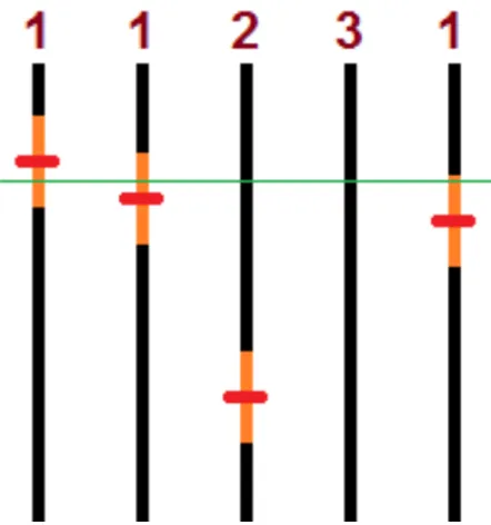
The second problem can be addressed by defining a window of sizews around the breaks detected by each log, and then checking not which logs are accusing a break at a given depthd, but which logs have a window overlapping depthd. If enough logs have breaks sufficiently near a given depth, as defined by their overlapping windows, and the sum of weightswof these logs are equal or greater than t, a break point is declared on the depth defined by the average of the depths of the logs involved, weighted by their respectivewweights. An example of this procedure can be seen in figure 3.2
Once the individual results are compared, and depths that pass the threshold test are declared as bedding contacts, we have an automated unified assessment of heterogeneities in the rock formation. This assessment is more accurate than one derived exclusively from the gamma ray log as it takes into account log characteristics other than organic matter content and grain size which are expressed in the gamma ray log.
26
Figure 3.2: Example showing the integration of break point results. Each vertical black line represents a log from the same well, where break points were detected at the red markers. The numbers on top of each log corresponds to the weight of that log. The orange sections on the logs represent the depths encompassed by the agreement window
ws. If we consider a weight of3to declare breaks, a break will be recorded in the final assessment on the depth corresponding to the mean depth of the three breaks crossed by the green line, as the sum of the three logs with breaks within that depth’s tolerance window is greater or equal than 3.
4
DOMAIN ONTOLOGY OF SEDIMENTARY FACIES
The branch of philosophy known as ontology, which is sometimes equated to meta-physics, is the field of study which deals with the nature and structure of reality. Aristo-tle defined ontology as the study of attributes intrinsic to things (GUARINO; OBERLE; STAAB, 2009). As such, an ontological study is not concerned with modeling reality under a perspective constrained by data and experiments, but with providing a description of the things present in the domain of interest. This means it is completely valid to study the ontology of dragons for example, even though dragons are fictitious beasts, they can be described in terms of concepts and relations.
In the context of computer science and software engineering, an ontology can be seen as a data artifact which specifies the concepts and relations that exist within the universe available for a given information system. In an ontology describing dragons for example, the concepts needed to describe our universe would includedragon,wings,scales,ability to breathe fire, hoard andhero, along with the required relations to link these concepts, such as possesses, guards and fights. These concepts and relations are organized into a hierarchical taxonomy, with drake for example being a subclass or specialization of
dragon. These general concepts can then be instantiated to refer to specific actors. A computational ontology has been defined as "a formal, explicit specification of a shared conceptualization" (STUDER; BENJAMINS; FENSEL, 1998). To fulfill these requirements this means the ontology should be written in a language that is machine readable, so it is formal. This allows the ontology to be queried and parsed by an appli-cation, which allows the system to answer questions such as"does an instance of dragon possesses a hoard?"by analyzing the actors involved and concepts that link them. Many languages exist today to encode these ontologies, such as OWL, KIF and OntoUML.
This definition also requires that our concepts and relations should interpreted cor-rectly and consistently so our specification can be explicit. The effective way to ensure this is to constrain the interpretation of the language used by the means logical axioms that allow the possible states of the universe in our specification to be modeled while also minimizing the possibility of modeling unintended, illegal states. For example, the relations fights and possesses can be differentiated by specifying the relation fights as irreflexive, intransitive and symmetrical and the relationpossessesas irreflexive, intransi-tive and asymmetrical. This is reflected in the languages described earlier, which tend to be based on predicates and first-order logic.
The last point made in the definition presented is that the ontology should be shared. This means the concepts and relations specified in the model should express a consensus instead of an individual view; since as a collection of structured knowledge, an ontol-ogy is only useful if information it models is agreed upon by all the users. Many top-level ontologies and domain ontologies have been created with this purpose of knowledge
shar-28
ing. Top-level ontologies such as DOLCE and UFO deal with describing the most basic concepts needed to represent and categorize various entities; they define for example, the difference between countable and uncountable subjects, concrete things versus abstract things.
A domain ontology can be defined as a collection of concepts and relations pertaining to a specific domain. Domain ontologies are usually extended from a known top-level ontology and deal with describing the concepts relevant to the domain of interest. We have for example the National Cancer Institute Thesaurus (NCIT) ontology, which defines over one hundred thousand terms related to the medical sciences. The core description data used in this work is backed by another domain ontology focused on the field of geol-ogy, this allows for standardized and unambiguous descriptions of the rock characteristics apparent in the samples.
When making core descriptions, geologists rely on drawings for expressing what they observe in the rock, since the available vocabulary for describing outcrops or rock sam-ples is in many cases incomplete or ambiguous. In a previous project, it was studied how to deal with this visual knowledge in order to provide the best support for captur-ing sedimentary facies descriptions for stratigraphic interpretation, keepcaptur-ing in mind that computers require propositional information for processing.
4.1
The Strataledge
R1Ontology
Lorenzatti in (ONTOLOGICAL PRIMITIVES FOR VISUAL KNOWLEDGE, 2010) proposed a hybrid representation approach for ontologies, which was demonstrated in a domain ontology for macroscopic description of sedimentary facies as a pair composed by an icon that visually resembles the visual aspect of sedimentary feature and a proposi-tional descriptor, as can be seen in figure 4.1.
Figure 4.1: Representation model of sedimentary facies built by a propositional term and a pictorial icon. The icon resembles the visual aspect of the facies. Source: (ONTOLOG-ICAL PRIMITIVES FOR VISUAL KNOWLEDGE, 2010)
Later on, Endeeper (STRATALEDGE: CORE DESCRIPTION SYSTEM, 2012) took advantage of this proposal and formalized an extensive domain ontology for facies de-scription of all types of rocks covering more than 750 geological features and 300 icons.
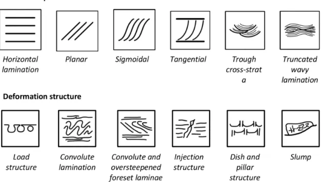
The ontology was developed following the principle of foundational ontologies (GUIZ-ZARDI, 2005) and it covers all the textural, structural, palentological and lithological aspects of igneous, metamorphic and sedimentary rocks, including the metassomatic, cat-aclastic and chemical less common types. The descriptive capability of the formal vo-cabulary provides the needed semantic content for the geologist to capture the aspects of the rock for stratigraphic interpretation. We can see in figure 4.2 a small example of the knowledge model of sedimentary features.
Figure 4.2: Examples of the rock facies domain ontology, showing the dual represen-tation of geological features. Source: (ONTOLOGICAL PRIMITIVES FOR VISUAL KNOWLEDGE, 2010)
The ontology originally proposed by Lorenzatti was further extended and refined by Carbonera in (CARBONERA, 2012) to support automatic interpretation of depositional processes. The author describes the features that define a sedimentary facies which are further used to discriminate the sedimentary units. These features were used by StrataledgeR in this work to segment and describe the core samples. A brief overview of
the sedimentary facies concept and its attributes as defined by the ontology is presented in Annex 1.
This extensive controlled vocabulary is embedded in an application for description of cores and columnar outcrops. The StrataledgeR system produces standardize
descrip-tions that are stored as records in a database, eliminating ambiguities and reducing sub-jectivity of the description process. This capability allows computer algorithms to process the information extracting automatic geological interpretation like those described in this work.
The Strataledge descriptions can then be exported in a XML format that allows for easy data processing, or as an SVG profile image file that can be shared for human in-spection. The core sample descriptions used in this work are expressed in the Strataledge format, which allows for easy correlation between the wireline logs and the core samples.
30
5
WIRELINE LOGS
Wireline logs are measurements taken from boreholes by using tools that may be low-ered in one at a time or as a series of sequentially connected tools. These measurements can be either taken during drilling by using logging while drilling (LWD) methods where the logging tools are integrated into the drilling head, or more commonly; after the drilling is done and the tools are lowered into the well one at a time or as a series of connected tools.
When done after drilling, the logging is commonly done while the well is still uncased, which means it has not yet been cemented and the pipe has not yet been inserted. This gives the tool access to the bare rock, which results in less obstructions and more precise readings. While not as common, logs made after the borehole is cased are still possible and are sometimes performed.
This chapter describes the most commonly used well logs (KRYGOWSKI, 2003) and the structure of the file used to record the data resulting from the logging process.
5.1
The LAS File
The Log ASCII Standard (LAS) file, developed by the Canadian Well Logging Soci-ety(CRANGLE, 2007) is currently the industry standard for storage of wireline log data and is organized as such:
1. A header informing the version of the LAS file.
2. A section containing metadata, such as the identity of well that is logged, its geo-graphical coordinates, elevation, logged depth, among others.
3. A section listing which logs are present in the file, each entry is composed of a mnemonic and an optional description.
4. A section containing the data itself, in the form of a list of space separated numerical values pertaining to each of the logs listed in the previous section at each of the logged depths.
5.2
Correlation Logs
The logs described in this section are usually used for correlation with other logs, as well as to differentiate between reservoir and non-reservoir formations.
5.2.1 Spontaneous Potential
Also known as SP, the spontaneous potential log measures the voltage from electrical currents resulting from the difference in salinities between water in the rock formation and the drilling mud in the well. As such, its values are can vary highly from well to well based on the drilling mud used. It can only be run in uncased wells and in the presence of water or water-based drilling mud.
This log can expresses the presence of a reservoir as a sharp change in value (either positive or negative) from an arbitrary yet stable baseline value. This log can also show the presence (but not the magnitude) of permeability in the rock formation. Depositional environment can also be inferred from the shape of the log curve. The presence of hydro-carbons or shale content in the rock formation will also cause a small deflection in the log value.
The mnemonic most often used for this log is SP, and the measurements are usually taken in millivolts (mV).
5.2.2 Gamma Ray
One of the most common logs, this tool measures the emission of gamma rays from naturally occurring thorium, potassium and uranium present in the rock formation. The tool may either take a single measurement from all these three elements, or discrete mea-surements from each one of them (in which case, it is referred to as a spectral gamma ray log). These tools have no restriction on cased or uncased boreholes, or the type of fluid present in the well.
Gamma ray measurements correlate to the amount of organic matter present in the rock formation. High values can therefore indicate a source rock, which is rich in organic matter, or a fracture where soluble uranium compounds have been deposited. Gamma ray readings are also highly correlated with shale content, and therefore, can be a good indicative of grain size.
The mnemonic used for this log is usually GR or some variation thereof. Spectral gamma ray logs may be divided in 3 logs, identified as THOR, URAN, POTA, or TH, U, K, based on the element being tracked. Measurements are taken in API or ppm.
5.2.3 Caliper
The caliper measures the diameter of the borehole, most commonly through the use of arms that extend from the tool. As with the gamma ray log, it is a very common log that has no operational constraints.
This log in particular has no direct correlation to rock type, and it is used mostly as input for environmental corrections on other logs.
The most common mnemonics used for the caliper log are CAL or CALI, measure-ments are taken in centimeters or inches.
5.3
Porosity Logs
The logs used in this section are mostly used to estimate the porosity of a given rock formation. It is important to note that none of these logs measure porosity directly, the estimation of porosity is usually obtained through the interpretation of the combination of two or three of these logs.
32
5.3.1 Sonic
This tool consists of a transmitter that emits sonic pulses that are then received by two or more receivers located on the same tool. The time differential between each receiver detecting the sonic pulse is called the transit time, or∆T. This tool can only be run in uncased boreholes containing a non-gaseous medium.
The sonic log is used in conjunction with neutron and density data as an estimator of lithology, it can also be a good indicator of the mechanical properties of the borehole, such as formation strength, permeability and porosity.
The usual mnemonic used for sonic logs is DT, and the measurements are taken in
µsec/ft orµsec/m. 5.3.2 Density
The tools in this category emit gamma rays from a chemical source towards the rock formation, two detectors in the tool count the number of returning gamma rays, which are related to the density of electrons in the rock formation.
Through combination with the neutron log, these density logs can be used to estimate lithology, gas presence, clay content and formation mechanical properties.
Density logs can refer to a variety of different log curves, such as bulk density (RHOB, DEN or ZDEN, measured in g/cm3 or kg/m3), density porosity (DPHI, PHID or DPOR,
measured in % or v/v decimal), density correction (DRHO, measured in g/cm3 or kg/m3) or photoelectric effect (PE, Pe, PEF, measured in b/e).
5.3.3 Neutron
The tool emits high energy neutrons from a chemical source which are slowed down by the nuclei in the rock formation. Two detectors in the tool count either the number of returning neutrons or gamma rays, which are inversely proportional to the amount of hydrogen residing in the rock formation. Since this hydrogen resides inside the pores of the formation, this measurement is related to the porosity of the rock.
This log can estimate porosity taking a specific lithology such as limestone as a base-line, corrections should be made to estimate porosity for other lithologies through the use of charts or other algorithms. By combining this log with density and sonic logs, it is possible to estimate lithology, presence of gas and clay content.
The common mnemonics for the neutron porosity log are NPHI, PHIN and NPOR, and the measurements are expressed as % or v/v decimal.
5.4
Resistivity
These logs measure the electrical resistivity of the rock formation, and can give an indicator of the fluid saturation in the rock formation.
5.4.1 Induction
The tool contains transmitter coils which induce an alternating current in the rock formation, the response is then sensed in both magnitude and phase by receiver coils built into the tool. This response is the conductivity of the rock formation, which is the inverse of the resistivity. This tool can only be run in an uncased borehole.
Induction logs can be used to calculate formation restivity, fluid saturation, diameter of invasion and geopressure.
Mnemonics associated to the curves generated by induction logging tools include ILD, RILD, ILM, RILM, LLR, SGRD and SFL, which are all measured in ohm.meter.
5.4.2 Laterolog
This tool creates a horizontal disk-shaped current around the borehole by focusing a low frequency current through the use of an electrode array. Resistivity can be measured by monitoring the current passing through the tool. This tool can only be run in an uncased borehole filled with water or water-based mud.
As with the induction logs, laterolog measurements can be used to calculate formation resistivity, fluid saturation, diameter of invasion and geopressure.
Mnemonics associated with laterologs are DLL, LLD, RLLD, SLL, LLS, RLLS and Rxo, which are all measured in ohm.meter.
5.4.3 Microresistivity
Also know ans Rxo, this tool forces an electrical current into the rock formation using electrodes mounted on pads which are pressed against the borehole wall. Some microre-sitivity tools focus the current using electrodes similar to the ones used in laterolog tools. This tool can only by run in an uncased borehole filled with water or water-based mud.
Rapid curve movement in this log can be an indicator of fractures. The relationship between microresistivity and other resistivity logs can be in indication of permeability. Microresistivity measurements can also be used to calculate flushed zone formation resis-tivity and water saturation. This log is also useful to identify very thin beds.
Microresistivity curve mnemonics include MNOR, MINV, MSFL and MLL, which are all measured in ohm.meter.
34
6
DESCRIPTION OF THE TESTING DATA
The greatest hurdle to overcome during this work was the obtention of quality testing data. Well data is highly confidential and therefore, going through the proper channels and obtaining the required clearance to work with the data takes time. Additionally, once the data is made available it is often useless for the process described in this work due to the datasets containing few logs, short or inexisting cored sections or simply due to the low quality of the data itself. Frequently the datasets acquired presented one extremely dominant lithology, usually sandstone, being over 80% of the cored section. Such bi-ased datasets make it difficult to create reliable lithology prototypes, as the less prevalent lithologies can present a number of samples that are not representative enough for reliable statistical analysis.
Another issue arises from certain lithotypes being highly variable when it comes to log responses due to their intrinsic properties. Heterolites, which are rock types charac-terized by the successive intercalation of thin layers of high and low grain size deposits are a good example of this. A section of rock may be characterized as a sand/clay hetero-lite and the log readings on this rock might be more similar to clay or sand depending on the ratio of clay to sand in this rock, which might lead to miscategorization. Evaporites such as anhydrite are also very troublesome due to interaction with water changing the chemical composition of the rock and drastically altering the resulting log readings. Oc-currences of anhydrite can therefore have highly unique log signatures depending on the environment on which they are situated. All these variations are common in real data and bring additional difficulties for the automatic recognition of rock types.
The data which is provided for scientific research also tends to be older, and while Strataledge provides a rich and well structured vocabulary with which to make the rock descriptions, the data captured in the field with direct access to the rock samples available for these experiments was not originally described with the semantic richness offered by Strataledge. Therefore, the Strataledge descriptions available for testing are translations of descriptions made using other less precise tools, which means the Strataledge toolkit is not being used to its full effect. Needless to say this confidentiality makes it extremely difficult to replicate the results of similar works since there is generally no access to their data.
Despite these issues, a suitable test case was found in a sedimentary environment where the cored section of the wells involved presented enough variability in lithotypes with enough samples to derive reasonable prototypes from once these lithologies were grouped.
The studied sedimentary succession was deposited in the Sergipe-Alagoas basin in northeastern Brazil. The wells used in this work belong to the Carmopolis field, where the depositional environment is interpreted as an alternation between fan deltaic systems
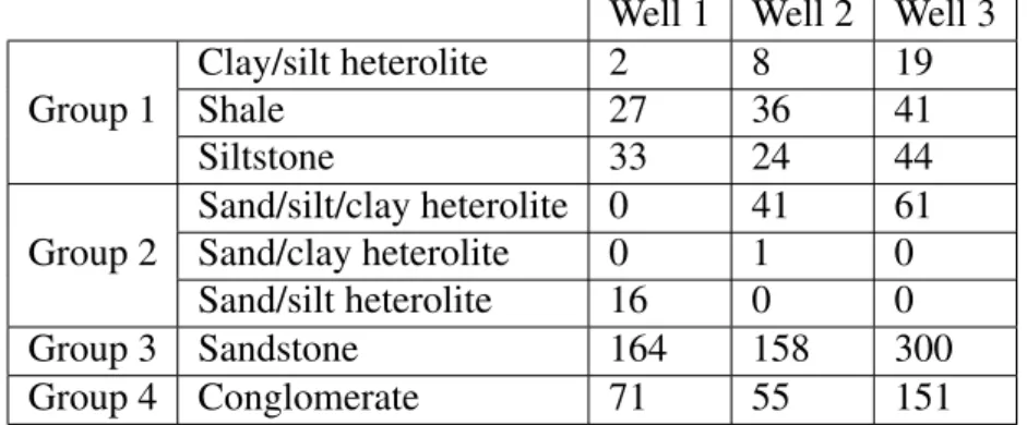
Table 6.1: This table shows the number of samples for each lithology in the three wells chosen for the test case.
Well 1 Well 2 Well 3 Group 1 Clay/silt heterolite 2 8 19 Shale 27 36 41 Siltstone 33 24 44 Group 2 Sand/silt/clay heterolite 0 41 61 Sand/clay heterolite 0 1 0 Sand/silt heterolite 16 0 0 Group 3 Sandstone 164 158 300 Group 4 Conglomerate 71 55 151
and associated alluvial fans and braid deltas prograding into lakes under arid/semiarid climate and increasing marine influence (AZAMBUJA FILHO et al., 1980) (CANDIDO; WARDLAW, 1985). In this environment, conglomerates, sandstones and mudrocks were deposited in fining-upward cycles. The reservoirs in this sedimentary unit are constituted of conglomerates and sandstones that occur at the base of the depositional cycles. Fining-upward amalgamated sequences of these cycles are interbedded with shales, marls, and calcilutites containing anhydrite nodules and stromatolitic laminites replaced by dolomite and anhydrite.
6.1
Testing Data Analysis
The method proposed was tested using real data from three exploration wells in the Sergipe-Alagoas basin. Each well had geophysical logs available measuring sonic transit time (DT), gamma ray (GR), resistivity (ILD), neutron porosity (NPHI), bulk density (RHOB) and density correction (DRHO); as well as core descriptions converted from hand-made descriptions into the Strataledge format. We can see this data plotted as scatter plots in figures 6.3 6.4 6.5. In these graphs, each box shows the samples present in each well plotted in a two-dimensional plane where each axis corresponds to one of the logs. In these graphs it is possible to see the high degree of correlation between certain logs, as well as how samples of the same lithology tend to be grouped together, this is especially noticeable in the conglomerates and sandstones in wells 2 and 3. A breakdown of the samples present in this data can be seen in table 6.1, it shows a clear dominance of sandstones and conglomerates among every well.
The difference in log signatures between certain lithotypes was determined to not be significant enough for reliable discrimination, so these lithotypes were grouped in four different groups by a geologist based on grain size and lithological similarity. The method then classifies each sampled depth as one of these groups, not as a specific lithology. The lithotypes present in the testing data were grouped as follows:
1. Group 1 - Claystone-Siltstone: Clay/silt heterolite, Shale, Siltstone
2. Group 2 - Siltstone-Sandstone: Sand/clay heterolite, Sand/silt heterolite, Sand/silt/clay heterolite
3. Group 3: Sandstone 4. Group 4: Conglomerate
36
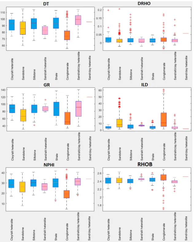
The grouped data can be seen plotted in figures 6.6 6.7 6.8. Box plots showing the differences of the log readings for each lithology can be seen in figure 6.1, box plots for the lithology groups can be seen in figure 6.2. These box plots show how the sampled values for each log is distributed in each lithology. The line in the middle of each box indicates the median value of that log for that lithology; the box represents the range in which 50% of samples are located; the "whiskers" extend to the value of the highest and lowest data points that are not outliers; outliers are marked by+sign and correspond to readings that are at least three scaled median absolute deviations away from the median. In these figures we can clearly see how the conglomerates have a very distinctive distribution compared to the other lithologies.
Additionally, a synthetic dataset was gracefully granted by the authors of (JEONG et al., 2014). This synthetic dataset presents three cases with 1600 samples each belonging to one of three artificial lithologies with two associated artificial log values. This data can be seen plotted in figures 6.9, 6.10 and 6.11. These cases come from scenario 3 described in (JEONG et al., 2014), which is the most complete scenario presented, where noise has been added to the data to better simulate the environmental conditions from a real well. Even in their most true-to-reality form, these graphs show readings with a much lower correlation, and much more well-defined groups than the real data presented.
Figure 6.1: Box plot of the log values for each of the lithologies present in the testing data. The logs present in this data are Gamma Ray (GR), Sonic (DT), Density (RHOB, DRHO) and Neutron (NPHI). The lithologies are color coded based on the group to which they were assigned. The sand/clay heterolite belongs to group 2 (pink), and contains only one sample. While the other two lithologies in group 2 seem to have contrasting signatures, this is due to the low number of samples on the Sand/silt heterolite not being representative enough to create an accurate model
38
Figure 6.2: Box plot of the log values for each of the lithologies present in the testing data. Notice the contrast in distributions between groups 3 and 4 (sandstone and conglomerates) and the other lithologies.
Figure 6.3: Plot of the samples contained in Well 1. Each square presents a scatterplot of two logs, the diagonal shows histograms of the distribution of each of the logs.
40
Figure 6.4: Plot of the samples contained in Well 2. Each square presents a scatterplot of two logs, the diagonal shows histograms of the distribution of each of the logs.
Figure 6.5: Plot of the samples contained in Well 3. Each square presents a scatterplot of two logs, the diagonal shows histograms of the distribution of each of the logs.
42
Figure 6.6: Plot of the samples contained in Well 1 grouped in the way described in this chapter. Each square presents a scatterplot of two logs, the diagonal shows histograms of the distribution of each of the logs.
Figure 6.7: Plot of the samples contained in Well 2 grouped in the way described in this chapter. Each square presents a scatterplot of two logs, the diagonal shows histograms of the distribution of each of the logs.
44
Figure 6.8: Plot of the samples contained in Well 3 grouped in the way described in this chapter. Each square presents a scatterplot of two logs, the diagonal shows histograms of the distribution of each of the logs.
Figure 6.9: Plot of the samples contained in the first synthetic dataset. Each square presents a scatterplot of two artificial logs, the diagonal shows histograms of the dis-tribution of each of the logs.
Figure 6.10: Plot of the samples contained in the second synthetic dataset. Each square presents a scatterplot of two artificial logs, the diagonal shows histograms of the distribu-tion of each of the logs.
Figure 6.11: Plot of the samples contained in the third synthetic dataset. Each square presents a scatterplot of two artificial logs, the diagonal shows histograms of the distribu-tion of each of the logs.
46
7
METHODOLOGY
Having the standardized core description and the corresponding geophysical logs, our method is divided into three steps: segmenting the log data into lithology intervals, build-ing lithological prototypes by matchbuild-ing core and log data, and finally assignbuild-ing lithologies to the segmented intervals by comparing them to the lithology prototypes. The method attempts to extrapolate rock data taken from cores ()which is rare and expensive), from log data (which is relatively cheap and abundant). A workflow of this process can be seen in figure 7.1, the steps taken in this workflow are detailed later.
Figure 7.1: This framework shows an overall view of our method for lithology detection, the processes involved and what data artifacts are used and generated.
7.1
Detecting Intervals
In order to extract lithological significance from wireline logs, the most intuitive way of doing this is to first segment the log into regions where the log readings stay within roughly the same value. This is the way geologists work while trying to identify rock for-mations from wireline logs, and our work attempts to emulate this process with automatic detection of these change points.
Starting from the assumption that a change in lithology can be characterized in the log record by a sudden change in the measured value, we detect these changes in lithology
using the work previously described in (GRACIOLLI, 2014) and presented in chapter 3. The assessment generated from this procedure can then be edited or not by the user using the program interface and the intervals defined by these break points are passed to the second part of the method, which will estimate the likely lithology of each interval based on the log values encompassed by each of them.
7.2
Determining Lithology
Once the intervals of interest have been determined, the log values measured at those depths can be analyzed and a lithological significance to the interval in question can be assigned. But first, a representation of each lithotype must be created and expressed in terms of numerical values, which can then be compared with the log readings taken at each interval.
With the standardized Strataledge core descriptions, the rock characteristics at any depth of a cored interval can be checked easily, this allows the parsing large amounts of data automatically. By checking the depth column in the log files, the rest of the core readings can be associated with a corresponding lithology if that depth at that well correlates to a cored interval, a prototypical log signature for each lithology can then be defined based on the readings taken at depths corresponding to that lithology. The set of logs and core descriptions used to create these prototypes is referred in this work as the training set.
The prototypes are created by calculating the average and covariance values between all available logs for each lithology. With these values, a log signature corresponding to a certain lithology can be expressed as a multivariate Gaussian distribution defined by the average vectorµand the covariance matrixΣ. Considering a matrixDm×nwhere each of
themrows corresponds to a sampled depth in the wireline log data, withnmeasured log values, the average vectorµcan be defined as expressed in the equation 7.1, and each of the values of the covariance matrixΣn×ncan be calculated as defined in equation 7.2.
During this step, the Bayesian prior for each lithology is also calculated. The prior of a lithologyLis expressed in 7.4, wherenis the number of samples of lithologyL, andm
is the total number of samples in the training data. This prior represents the probability for a data point belonging to a given lithology before being analyzed. This prior is useful to give more weight to lithologies that are common in the testing data.
µ= [ m X i=1 Di,1 m , m X i=1 Di,2 m , m X i=1 Di,3 m , ..., m X i=1 Di,n m ] (7.1) Σj,k = m X i=1 (Di,j−µj)(Di,k −µk) m (7.2) pdf(x, µ,Σ) = q 1 (2π)k|Σ|exp(− 1 2(x−µ) T Σ−1(x−µ)) (7.3) P(L) = n m (7.4) updf(x, µ,Σ) = m X i=1 pdf(xi, µi,Σ(i,i)) m (7.5)
Each interval defined in the first step can then be checked to determine which lithology is the best fit for each interval. This is done by checking every point inside the interval