Open Research Online
The Open University’s repository of research publications
and other research outputs
Mining credit card data
Thesis
How to cite:
Blunt, Gordon (2002). Mining credit card data. PhD thesis The Open University.
For guidance on citations see FAQs.
c
2002 The Author Version: Version of Record
Copyright and Moral Rights for the articles on this site are retained by the individual authors and/or other copyright owners. For more information on Open Research Online’s data policy on reuse of materials please consult the policies page.
UNCT6
Mining credit card data
Gordon Blunt, BA
Department of Statistics
Faculty of Mathematics and Computing
The Open University
Submitted for the degree of Doctor of Philosophy February 2002
o,
LO.002OAbstract
Data mining is the process of finding interesting or valuable structures in large data sets. It is a modern discipline, and takes ideas and methods from statistics, machine learning, data management and other areas. In many ways, it is similar to exploratory data analysis, although the size of current data sets distinguishes between data mining and standard exploratory data analysis. Data mining can pose novel challenges because of the amount of data to be analysed.
This thesis is concerned with modelling different aspects of credit card holders' behaviour and detecting patterns in the ways customers use their card accounts. A review of the literature on consumer purchasing behaviour and data mining is given, and for the latter the differing viewpoints of the statistical and the computer science communities are discussed.
Two types of models are examined: descriptive models, which describe how customers have been observed to behave; and predictive models, which predict how customers are likely to behave in the future. Both types of model are applied to the main types of credit card use: repayment behaviour and transactional behaviour. Relationships between the two different sorts of behaviour are described, and models are examined which can link the two. Some valuable insights and discoveries of potential commercial value are described.
Simple graphical tools are used to illustrate the unearthing of unexpected patterns and relationships, and it is shown how more sophisticated modelling can build on such discoveries.
Acknowledgements
I would like to thank my supervisor, Professor David Hand, for his constant
guidance, encouragement and patience. I would also like to thank Drs Niall Adams
and Mark Kelly for their help and support.
I am grateful to Barclaycard for allowing me to use data for this work, and partly
funding my research; and to Sandra Linney and Alex Kells for helping with data
extraction.
Finally, I would like to express my gratitude to Judy, for her patience and tolerance
INTRODUCTION AND REVIEW OF PREVIOUS WORK.!
1.1 Aim of this thesis...2
1 .1.1 Structure of the thesis...3
1.2 Modelling consumers' purchasing behaviour...5
1.2.1 Introduction ...5
1.2.2 The pattern of consumer purchases ... 5
1.2.3 Random effects models - univariate parameterisations...5
1.2.4 More complex approaches...8
1.2.5 The econometric approach...10
1.3 Data mining ...11
1.3.1 Introduction...I I 1 .3.2 Data mining and visualisation ...13
1.3.3 Data mining from a statistical perspective...14
1.3.4 Data mining and 'data dredging' ...22
1.3.5 Data mining from a computing perspective...22
1.3.6 Examples of data mining...29
1.3.7 Data mining tools ...36
1.4 Summary...40
2 THE HISTORY OF THE UK CREDIT CARD MARKET ...41
2.1 Introduction ...41
2.1.1 Credit cards and other cards ...42
2.1.2 The credit card market cycle...44
2.2 The development of the UK credit card market...47
2.2.1 Credit card profitability...50
2.2.2 Growth in credit card activity...51
2.2.3 Recent changes in the UK credit card market...53
2.2.4 Multiple card ownership...59
2.3 Conclusions: the future...60
3 BARCLAYCARD CREDIT CARD DATA ...64
3.1 Introduction ...64
3.1.1 Account history ...65
3.1.2 Transaction history...67
3.2 Other data issues...70
3.2.1 Customers 'lost' from the sample...70
3.2.2 Selecting only those customers present for the whole of the period...72
3.2.3 New customers ...72
3.2.4 The sample that remained...73
3.2.5 Negative balances...73
3.2.6 Caveats...75
4 REPAYMENT BEHAVIOUR - DESCRIPTIVE MODELS ...76
4.1 Introduction ...76
4.2 Selecting a suitable classification scheme ...79
4.2.1 Use of linear regression to predict the amount of interest paid...79
4.2.2 Number of occasions on which interest is incurred...81
4.2.3 Devising a suitable classification schema...82
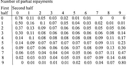
4.2.4 Patterns of partial repayment...84
4.2 . 5 Patterns of partial repayment - 'real' partial repayers...93
4.2.6 Patterns of partial repayment - late payers...95
4.3 Conclusions ...96
SREPAYMENT BEHAVIOUR - PREDICTIVE MODELS ...99
5.1 Introduction ...99
5.1.1 Classification of repayment behaviour...100
5.1.2 Using a simple assessment table to judge our predictions...100
5.1.3 Linear regression, broader definition of partial repayment...103
5.1.4 Linear regression, 'real' partial repayments ...106
5.1.5 Linear regression, forgetful repayers only...108
5.2 Classical linear discriminant analysis...108
5.2.1 Introduction...108
5.2.2 More precise definitions of partial or forgetful payers ...111
5.2.3 Conclusions...112
5.3 Separation of the classes...114
5.3.1 Discriminant analysis plots to investigate separability...114
5.3.2 Separability - summary...116
5.4 Nearest neighbour methods ...116
5.4.1 Introduction...116
5.4.2 Choice ofk...116
5.4.3 Relationship between k and the threshold...120
5.4.4 Choice of a suitable distance metric ...120
5.4.5 Conclusions: k-nearest neighbour methods ...121
5.5 Other types of discriminant analysis...123
5.6 Conclusions ...124
6 PROFITABILITY GAINS FROM DISCRJMINANT ANALYSES...126
6.1 Cost-benefit analysis...126
6.1.1 A general equation for assessing profitability... 127
6.1.2 Analysis of revenue and costs...128
6.1.3 Real partial repayers results...130
6.1.4 A random sample of customers from the whole file...131
6.1.5 k-nearest neighbour methods...132
6.2 Conclusions ...133
7 TRANSACTION DATA- DESCRIPTIVE MODELS...134
7.1 Introduction ...134
7.2 Summary information...135
7.3.1 Relationships between sectors...141
7.4 Frequency of use and amounts spent ...145
7.5 Seasonality...148
7.6 Data quality and data distortion...149
7.7 Petrolstation transactions...151
7.7.1 Introduction...151
7.7.2 Petrol station spending...153
7.7.3 Intra weekly patterns ... 155
7.7.4 Conclusions increasing value of petrol station transactions...156
7.7.5 Individual transactions...156
7.7.6 Modelling the probability that a customer rounds ...164
7.7.7 Assessing goodness of fit...167
7.7.8 Condensing the transaction size - modulo pence amounts...168
7.7.9 Simple geometric model...171
7.8 Logistic regression...172
7.8.1 Introduction...172
7.8.2 Results...173
7.8.3 Rounders and non-rounders...174
7.8.4 Potential covariates...175
7.8.5 Conclusions about logistic regression...176
7.9 Conclusions ...176
8 CHARACTERISATION OF TRANSACTION PATTERNS ...178
8.1 Introduction - taxonomy of spending behaviour...178
8.2 Number of transactions...179
8.2.1 The negative binomial distribution...179
8.2.2 Numeric predictions for two of these sectors...182
8.2.3 All sectors...184
8.2.4 Conclusions...185
8.3 Transaction amounts by sector ...186
8.4 Number of sectors used, by sector...190
8.4.1 Introduction...190
8.4.2 People sector occasions'...191
8.4.3 Sector use by all other sectors ...193
8.4.4 Number of sectors and transaction amounts...196
8.4.5 Conclusions about a taxonomy of spending behaviour...197
8.5 Graphical models...198
8.5.1 Spurious links - chemists and supermarkets...202
8.6 Sectors used and their probability of use ...203
8.6.1 Introduction...203
8.6.2 Conditional probabilities ...204
8.6.3 Odds ratio...208
8.6.4 Association rules ...211
8.6.6 Conclusions about association rules . 217
8.7 Number of sectors and amounts spent ...219
8.7.1 Distribution of transactions by number of sectors used...223
8 .8 Principal components, and cluster analyses...225
8 .9 Conclusions ...227
8.9.1 Characteristics of spending behaviour...227
8.9.2 Conclusions about a taxonomy of spending behaviour...228
9 TRANSACTION DATA- PREDICTIVE MODELS...231
9.1 Introduction ...231
9 .2 Predicting peoples' total spend...231
9.2.1 Using the sectors in which they spend...231
9.2.2 Discussion of this model...233
9.2.3 Transformations...235
9.2.4 Predicting one year's spend from the previous year...235
9.3 Predicting individual sectors' spend...237
9.3.1 Linear regressions...237
9.3.2 Other predictor variables...239
9.3.3 Number of transactions...239
9 .4 Conclusions ...241
10 LINKING TRANSACTION AND REPAYMENT BEHAVIOUR ...243
10.1 Introduction...243
10.1.1 Segmentation versus clustering ...244
10.1.2 Amount spent and number of partial repayments...245
10.2 Tree based models...247
10.2.1 Introduction...247
10.2.2 Number of transactions and repayment behaviour...248
10.2.3 Predicting transactions the following year...249
10.2.4 Conclusions...250
10.3 Differences between full payers and borrowers...251
10.3.1 Proportions using each sector...251
10.3.2 Amounts spent by full payers and borrowers...252
10.3.3 Interest and number of sectors used...254
10.4 Conclusions...258
11 CONCLUSIONS AND FUTURE WORK ...260
11.1 Conclusions...260
11.1.1 What we learned...260
11.1.2 What the business is doing differently...264
11.2 Future work...265
11.2.1 Repayment behaviour...265
11.2.2 Spending behaviour...267
11.2.3 General ...268
Chapter 1
1 Introduction and review of previous work
The UK credit card market is in a state of flux. This change is being stimulated by a variety of causes, including new competition, new technologies, increasing customer awareness, and tougher customer requirements. Existing players are faced with problems of attracting new customers in the teeth of greater competition and of retaining customers who may be tempted to move elsewhere. At the other end of the spectrum, card issuers seek to encourage customers to use their cards instead of using alternative payment methods.
Growth has been strong since credit cards first appeared in the United Kingdom (BBA, 2001), although the market was slowing by the early 1990s. In the second half of the decade, with the arrival of new types of competition, credit card growth more than doubled: from less than 7% a year to more than 15% a few years later. Furthermore, there were perhaps 30 different credit cards in circulation in 1990, whereas today's figure is closer to 2,000 (MoneyFacts, 2002).
The impact of these massive changes is described more fully in Chapter 2, but the long established credit card issuers needed to make huge changes to the way they work, the products they provide, and the way they use their data. Some of the data sets are large - in 2000, there were almost 50 million credit cards in circulation, customers spent more than £95 billion on 1.5 billion transactions, and borrowed more than £35 billion (BBA, 2001).
1.1 Aim of this thesis
The aim of this thesis is to model aspects of and detect patterns in, the way customers use their credit card accounts. In particular, we look at repayment behaviour and transaction behaviour, and use a variety of tools to do so. Some of these come from a statistical background; some from those used by the data mining community.
We will examine two kinds of models: 'descriptive models' and 'predictive models'. Descriptive models describe how customers have been observed to behave. In particular, our aim here is to divide the population of customers into qualitatively distinct behavioural subgroups. In contrast, predictive models predict how customers are likely to behave. Here, we make a further distinction between predictive models which
(1) permit us to choose people who will be most likely to exhibit particular types of behaviour (e.g. often fail to pay their account in full; or the total amount of interest they might pay in their first year),
(2) predict expected future behaviour so that it can be modified (e.g. sometimes, but not often, fail to pay account in full; perhaps with the intention encouraging customers to spend more widely).
Both type 1 and type 2 predictive models are useful for marketing purposes. We call them, respectively, 'first order' and 'second order' models.
Data mining generally deals with messy, distorted data, possibly from samples that have not been properly constructed, and if the formal inferential tools of statistics are
applied, their results may need to be viewed with some caution. One consequence of this is that sophisticated statistical model building tools are likely to be of less relevance in a data mining context. Many of the latter (for example bootstrapping or general linear models) will not result in markedly better models than simpler approaches (e.g. linear regression), yet are likely to take much longer to produce, given the size of the data sets involved. In many ways, data mining has similarities to exploratory data analysis, although the size of current data sets distinguishes between data mining and standard exploratory data analysis, as described by Tukey (1977).
We discuss the distinction between patterns and models in Section 1.3: a model is an overall summary of a set of data, or subset of data; a pattern is a small scale feature of a data set. In this work we are mainly seeking to model peoples' behaviour, and that is the reason it is appropriate to use a relatively small (by data mining standards) sample of 10,000 customers and a million transactions. We describe these data more fully in Chapter 3.
1.1.1 Structure of the thesis
After this introduction, the remainder of the chapter reviews previous work, and this is split into two parts - the first describes the modelling of consumers' purchasing behaviour and the second describes data mining. Chapter 2 is a review of the current
state of the credit card market in the UK and Chapter 3 gives details of the data set
on which our analyses have been undertaken.
In Chapter 4, we describe several ways to define characteristics of repayments to credit card accounts. Customers can repay any amount between the full amount and
the minimum requested by the card issuer (Chapter 2 gives more details). In Chapter
5, we describe a number of ways to predict such behaviour in the future, and in
Chapter 6, we estimate the revenue such activities can generate.
Chapter 7 introduces spending behaviour, and we describe characteristics of how people use their cards for spending in different trade sectors. We also describe data quality and data distortion, and explain one sector - petrol stations - in detail, and model some unexpected behaviour in that sector. In Chapter 8 we describe a taxonomy of spending, give parsimonious models for certain characteristics of spending, and describe how different sectors are related. In Chapter 9, we describe how to predict future spending from current data.
In Chapter 10, we link the theme of Chapters 4 to 6 with that of Chapters 7 to 9. In other words, we link repayment and spending behaviour, whereas in the earlier chapters we considered the two aspects of credit card use separately. We show how they are related, which they must be (in some sense) because they are different aspects of customers' use. Often, the relationships between the two types of behaviour may not be immediately obvious.
Finally, in Chapter 11, we give our conclusions, and present directions for future research.
Most of the work that follows describes our attempts to construct models of behaviour, and to find patterns in the data. To do this, we will use a range of techniques, including linear discriminant analysis, k-nearest neighbour analysis, principal component analysis, linear and logistic regression, visualisation, graphical models, and association analysis.
1.2 Modelling consumers' purchasing behaviour
1.2.1 Introduction
Much work has been done on aspects of modelling consumers' spending behaviour, particularly the purchasing of packaged grocery brands. There are two main strands to this, one from a statistical, and the other from an econometric, viewpoint. We describe both of these in Section 1.2, and in Chapter 8, we use the methods described in the next section to model the number of transactions in different trade sectors.
1.2.2 The pattern of consumer purchases
There are many ways in which we can describe the spending of credit card holders: for example, the number of transactions made by each customer (in a specified time), or the total amount represented by these transactions, or perhaps the time of year at which they are made. The first and third of these could give us a fourth - that of frequency of purchase, which may vary by customer, by sector and by the time of year. In this section, we describe work others have done to model the number of purchases of packaged goods. This has a close analogue with our data, especially the number of transactions per customer per sector.
1.2.3 Random effects models - univariate parameterisations
Early work described the use of the Negative Binomial Distribution (NBD) to model
consumer purchases (Ehrenberg, 1959). This distribution has several characteristics
shared by the consumer panel data that Ehrenberg used - it is always positively skewed, has only one mode, often at zero, and leads to a 'reverse J' shaped distribution. Our data show similar characteristics, although typically the tail of our distributions is longer than those shown by Ehrenberg. He used the NBD because it
fitted well the consumer purchasing data sets he examined. An appealing feature was also the relative simplicity of the distribution, because it is completely specified by two parameters. Two further assumptions were made: that the purchases of any particular customer in successive time periods were independent random samples from a Poisson distribution; and that the distribution of the average rates of purchasing ji of different consumers should be proportional to a , distribution with
2k degrees of freedom. Here, k is the exponent of the NBD.
Chatfield et al. (1966) noted another simple distribution that would fit consumers' purchasing data - the Logarithmic Series Distribution (LSD), and realised that in many situations, the LSD and NBD give almost equivalent results. However, for some 'heavily-bought products' Chatfield noted that the fit to the LSD 'is not very good'. We will demonstrate that the NBD suffers a similar problem for our more heavily used sectors, albeit providing a very good fit over most of the data - usually with more than 95% being explained. The NBD model only applies when purchasing behaviour is stationary, and most of our data, over the short period at our disposal, are effectively stationary.
The same authors, in a later paper, (Goodhardt et al., 1984) expanded the model's basic form into the Dirichlet model, which gives a multivariate Beta or Dirichlet distribution across different consumers. It differs from the earlier models, which were for individual brands, but this approach can be used for a product class as well (i.e. multiple brands). Like the NBD, this approach models a stationary market and it introduced some concepts similar to those that will appear in this work. These are as follows.
Penetration is the proportion of the population buying a particular brand, which here becomes the proportion of credit card customers spending in a particular sector with their credit cards. Indeed, Chatfield (1986) refers to 'purchase occasions'.
Repeat buying is the purchase of brand X in subsequent time periods, and here becomes the subsequent use of the same sector.
Purchase frequency per buyer. This is as obvious as the description implies.
The distribution of brand purchases becomes one of several ways that we can use to describe customers' behaviour, such as the number of weeks in which a particular sector is used, or the amount spent in a sector.
Total product purchases becomes total number of transactions made by each
customer.
Goodhardt et a!. (1984) use the term 'Dirichlet model' as shorthand for the NBD-Dirichlet model, and the NBD is still an important part of the approach, and the authors simplify the calculations to those of a Beta-Binomial distribution. For a
specific brand j, with brand share a'/S in product class S, the probability of making
r1 purchases of brandj, conditional on n purchases of the product class having been
made (r ^ n) is given by the Beta-Binomial distribution
B(a1,S—a)
Wrigley and Dunn (1985) extended the NBD and Dirichlet models to encompass covariates; Davies and Pickles (1987) to trip timing and store choice of grocery shoppers; while Romaniuk et al. (1999) applied it to the use of products, particularly shampoo. Queen (1999) used a multiregression dynamic model, which followed earlier work on a generalisation of the Dirichlet model to partially segmented markets. Segmented markets can be defined as follows. Suppose a market consists
of m brands {l, ..., m}, which are sold to n types of consumer {T(l), ..., T(n)};
associated with T(i) is a type set C(i) c {1, ..., m}, 1 ^ n ^ n, containing all of those
brands which T(i) chooses. If n = 1, so that there is a single type of purchaser for the
whole market: the market is homogeneous. If the type set {C(1), ..., C(n)} forms a
partition of {1, ..., m}, the market is said to be segmented, otherwise it is said to be
partially segmented. The analogue in this work is that credit card customers can use their card in a subset of trade sectors, and not use it at all in others.
All of the approaches just described have equivalents in our data, particularly in the number of transactions made, and their frequency.
1.2.4 More complex approaches
Allenby et al. (1998) and Allenby and Rossi (1999) model the heterogeneity in peoples' purchase decisions, primarily by using a Bayesian approach, and conclude that such modelling is preferable to 'classical approaches to modeling heterogeneity' because much of the influence on a particular consumer is 'not well represented by summary statistics'. Their hierarchical approach allows for parameter estimation at what they call the 'disaggregated level', i.e. to smaller groups of consumers. Foekens et al. (1999) use varying parameter models to try to estimate the dynamic effects of promotions, as do Bhargava and Sargan (1984), although the latter applied
their techniques to income data, rather than purchasing behaviour. Dekimpe et al. (1999) used unit root based econometric models to estimate the long and short run effects of price promotions.
Kamakura and Russell (1989) used a latent variable approach to market segmentation, based on the assumption that consumers can be allocated to a small number of segments, 'each characterized by a vector of mean preferences and a single price sensitivity parameter'. Latent class models assume that homogeneous groups of consumers exist, and can be modelled. The authors allowed brand preference and price sensitivity to affect the choice among competing brands.
Chiang et al., (2001) describe weekly purchase data in several packaged grocery product categories, using hazard functions, and concluded that short term promotional activities have little effect on the timing of consumers' purchases. The emphasis of their work is the time between successive purchases, and whether or not that can be influenced by promotional activities. Allenby and Lenk (1994) used logistic normal regression, although they focused on 'brand choice probabilities', which is not really relevant to our work because card holders can buy any product or brand they choose. The analogue for our data is that people may choose, or not, to use their card (or other means of payment) for any particular purchase. In this work, we have little information on the proportion of a consumer's total spending that we see on our credit card, so will not pursue this idea, although a development for future analysis is to look at a customer's credit and debit card transactions when the cards are from the same bank.
1.2.5 The econometric approach
Leszczyc and Bass (1998) review recent models on consumer brand choice and include, in passing, some of the sources we have mentioned. However, their main thrust, along with much of the econometric literature, is to move away from the parsimonious specifications of the NBD approach, which characterises much of the work we described in Section 1.2.3.
Allenby and Ginter (1995) describe a way of segmenting markets, using a Bayesian random effects model, with consumers whose response to particular offers can be defined as 'extreme' in some way. They used customer preferences from a market research study, rather than actual behaviour, for this approach. A possible drawback is that typically 90% of a population lies outside the extremes, but the authors suggest the technique will assist in product design, rather than marketing to the population. They believed that people at the extremes would be more likely to switch to different products, and thus have the most extreme values for product attributes, which could guide new product design. In our data set, use of this type of market research data is not practical, because most of our data are behavioural, and derived from peoples' use of their cards. In many cases, demographic details are not stored, or only updated spasmodically, and are thus of limited use. In the cases where relatively full data are available, it is likely to be among newer customers, but at any one time, new customers typically comprise only around a tenth of the file, which is of little practical use if we seek to model aspects of all customers' behaviour.
Allenby et al. (1999), sought to model 'interpurchase' times of individual customers of an investment brokerage firm by means of a generalised Gamma distribution. A
sentence in the introduction illustrates that perhaps the authors consider the 'traditional' (i.e. more parsimonious) statistical approach to be flawed: 'firms have been forced to use statistical models of purchase data that by necessity ignore competitive effects and unobserved customer behaviour (e.g. purchases of competitive products)'.
1.3 Data mining
1.3.1 Introduction
Data mining has been defined as the 'discovery of interesting, unexpected, or valuable structures in large data sets' (Hand and Blunt, 2001) and as 'the application of algorithms for extracting patterns from data' (Fayyad et al., 1996b). The latter authors, in a later paper (Fayyad et al., 1996c) defined Knowledge Discovery in Databases (KDD) as 'the overall process of discovering useful knowledge from data, and data mining refers to a particular step in that process'. We will use the first definition, rather than the narrower one, because we view data mining as more than the development and use of algorithms. It must involve analysts with both domain and statistical knowledge, otherwise the findings from any data mining exercise could be flawed.
Interest in data mining as a research topic has mushroomed in recent years. A search of the Institute for Scientific Information's 'Science Citation Index' and 'Index to Scientific and Technical Proceedings' found 39 references to papers mentioning 'data mining' in 1996, but that had risen to almost 1,000 by 2001. Many of these are from computer science - Mackinnon and Glick (1999), for example, list a hundred references, half of which are in publications concerned with computer databases.
There are many general introductions to data mining, and we discuss those from statistical and computer science backgrounds in Sections 1.3.3 and 1.3.5 respectively. Some texts are also written for the business user, and concentrate more on potential business applications of data mining, and less on methodology. Two recent examples are Berry and Linoff (2000) and Rud (2001).
We draw a distinction between patterns and models, and use the definition of Hand, Blunt, Kelly and Adams (2000). A model is an overall summary of a set of data, or subset of data, so it is thus the 'standard' statistical use of the term. It could be, for example, a linear regression model, or a conditional independence graph, or one of many others. In this work we are mainly seeking to model peoples' behaviour, and that is the reason it is appropriate to use a relatively small (by data mining standards) sample just over 10,000 customers. In another sense, ours is not a small data set, because there were more than 1,000,000 transactions in the two years for which we had data. We describe these data more fully in Chapter 3.
Apattern is a local structure, referring to a small number of objects, where 'small' is
context dependent. An example in our case could be the 0.5% of petrol station
transactions that are for amounts of more than £100 (the 99th centile of this
distribution is just over £50). We describe transactions in this sector in some detail in Chapter 7. Another could be the 0.2% of customers who maintain a 'negative balance' for a whole year. We describe our approach to dealing with these customers in Chapter 4
1.3.2 Data mining and visualisation
An important aspect of any data analysis is visualising the data. The power of visualisation methods derives from the ability of the human eye to perceive patterns, which is what it evolved to do. We will describe, in many parts of this work, different ways of looking at data, and the importance of using appropriate methods. In this instance 'appropriate' means that the structure or interesting or useful aspects of the data become apparent. We will also give examples of how difficult it can be to select the most suitable methods, especially with large data sets, and show that simple techniques, such as scatter plots or histograms, may be suitable, providing they are used in a sensitive way. In general, some sensitivity and awareness of the properties of the methods are needed in order to avoid mistaken conclusions. Examples in Chapter 8 show that truncated histograms can reveal structure that is completely concealed in histograms showing all of the data. We also show how an increase in median spend per sector, as the number of sectors increases, conceals the fact that the majority of customers had relatively little spending. We will also show how, if used insensitively, the analyses themselves can conceal structures.
Hand and Blunt (2001), said 'Visualisation is very important in data mining, and some highly sophisticated tools, which can process vast datasets and which are based on supercomputers have been developed. Of course, visualisation in huge data sets is but the natural development of older graphical methods, many of which are still effective in quite large data sets - though sometimes care has to be exercised. [...] Perhaps we should also note the advantage of graphical and visualisation tools in helping to convince (possibly non-numerate) senior management of the reality of the discoveries that have been made.'
Others who have written at length about the importance of visualisation are Tufte (1983), Chambers et al. (1983) and Cleveland, (1993). It was also an important part of works such as Keim and Kriegel (1997), Cox et at. (1997) and Mackinnon and Glick, (1999). One of our aims in this thesis is to illustrate how these 'standard' (and, indeed, classical) graphical methods can be applied in data mining.
1.3.3 Data mining from a statistical perspective
Many authors have written on this subject, for example Chatfield (1995), Elder and Pregibon (1996), Glymour et al. (1996, 1997), Huber (1997), Hand (1998a), Mackinnon and Glick (1999), Hand (2000b), Smyth (2000) and Hand, Mannila and Smyth (2001). The last of these is an interdisciplinary text, and could appear in our review from a computing, as well as a statistical, perspective. Several themes run through these sources, as follows.
Parzen (1997), in his consideration of the relationship between the statistical sciences and data mining, defines 'core statistical research' to be 'about mathematically synthesising ideas drawn from many analogous applications'. He proposed the use of an alternative name 'statistical methods mining', and suggested, like Fayyad et al. (1996c) that data mining cannot take place without statistics.
(1) Size of the data sets
Many huge data sets exist today that contain with terabytes of data. For example, we refer below to the SKICAT analysis of Fayyad et al. (1996a) that has three terabytes of astronomical data. Hand, Blunt, Kelly and Adams (2000) give several examples, such as the 7 billion transactions a year made in Wal-Mart stores, and Pregibon (2000) describes the 70 million telephone long distance calls handled a day by
AT&T. Statisticians have not generally confronted data sets with millions of cases, and tens of thousands of variables, mainly because such data sets are relatively recent.
Several problems arise as a direct consequence of data sets this large, especially when we need to analyse them, and Wegman (1995), Glymour et al. (1996, 1997), Huber (1997) describe some of the problems that can arise. Hypothesis tests may not work, because they can lead to the rejection of models no matter how closely they seem to fit the data. We give examples of this in Chapters 4 and 7, on repayment behaviour and petrol station transactions respective]y. Traditionally, statisticians have used a values of 0.05 or 0.01, and these might be wholly inappropriate with massive data sets (Glymour et al. (1997) say that 'this point is of fundamental importance for data miners')
Huber (1997) describes the fact that standard errors and other tests of significance might not make sense when applied to 'samples of convenience' or 'opportunistic' data sets. Many data sets in the data mining literature appear to be of this nature, as pointed out by Glymour et al. (1997) and Hand and Blunt (2001). Greenfield (1994) gave examples of researchers - in disciplines other than data mining - who experienced problems because they collected data without sufficient thought about how the objectives of their research could be formulated in terms of a statistical problem. In data mining, similar problems are likely to arise because data are often taken as an opportunistic sample from a large data set and presented to the analyst. She or he may have no influence on how the data are derived, or how the sample is constructed.
Parameter estimation can also be problematic (Glymour et al., 1997). Classical statistics treats the parameters as fixed but unknown, and Bayesian statistics provides a framework for estimating the distributions of parameters, when the data under investigation come from a sample that is governed by probability distributions. These assumptions are often violated in data mining contexts. Also, as Hand (2000b) pointed out, the data miner's main concern may lie elsewhere, especially with the speed of the algorithm used to produce a model. There may well be an emphasis on sequential algorithms where only a single pass through the data is required.
(2) Data mining can be pattern focused rather than model focused
This relies on the definition of patterns as local, often small, structures (Hand, Blunt,
Kelly and Adams, 2000) or local dependencies (Glymour et al., 1997). This is distinct from models, which are overall summaries of the entire data set (Glymour et al., 1997, Hand, Blunt, Kelly and Adams, 2000). Data mining, and the methods used in a particular application, are driven by the needs of the application itself. If patterns are of importance (for example in plastic card fraud detection) then there might be no alternative but to search for all occurrences of particular patterns in the data. In the case of credit cards, fraudulent transactions occur very infrequently: 0.17% of credit card turnover in the UK in 2000 (BBA, 2001), but it is the industry's objective to prevent every such transaction, if possible.
(3) Problems with causal inference
As noted by Glymour et al. (1996), 'causal inference from uncontrolled convenience samples is liable to many sources of error'. Statisticians are well aware of this - the
Problems arise from three main areas: latent variables, sample selection bias, and model equivalence.
Latent variables are unrecorded features that affect variables that are recorded in the database, and whose variation influences some of the recorded variables. The result can be an association between two variables that is not a result of the direct association between the features themselves. For example, we might find that our data indicate a relationship between the amount a customer spends in two particular trade sectors. However, a possible explanation for this relationship would be that shown in the following graphical model, where spending in the two sectors is conditionally independent given the number of children. Our data set does not contain this last variable, so it would not be possible to identify that the correlation was spurious.
No. of children
/
supermarkets Clothing shops
Sample selection bias can occur when data are not a properly specified sample (see the penultimate paragraph in (1) above). Whether selection bias is important is dependent on the objectives of the analysis - if we seek to make inferences to an underlying population, any sample bias can invalidate our results. For example, to
select a 10% sample, it is easy to select every 10th case, starting from a random point
in the first ten. However, if there is some relationship between successive members then there is a danger that there could be some periodic structure in the list. The data
we describe in Chapter 3 were not affected by this, but shortly after we extracted our sample there were several 'upgrade' programmes. Customers were given different cards, depending on their behaviour. Tranches of account numbers were allocated sequentially because of these programmes, and had we taken our sample later than we did, we would have had to have taken note of this in the sampling method we used.
Model equivalence occurs when it is possible to find different models that all adequately fit the data, and which could have 'quite distinct causal implications' (Glymour et al. 1996, 1997). A procedure that arbitrarily selects one (or a small number) of these models can lead to different inferences. Huber (1997) also notes that models can be distorted by selection bias.
One data mining technique outside 'traditional' statistics may be prone to confusion between correlation and causality: that of association rules, where the notation itself could be the source of misunderstanding. Association rules were defined in I-land, Blunt and Bolton (2001) as follows. Let Vbe a set of attributes, corresponding to the set of all possible items that can exist in a database. A transaction, T, is a subset of
V. An association rule, R, is a pair (A, B), where A is a subset of V, and B is
(usually) a single element of V, not in A. A is often called the antecedent of the rule, and B the consequent. A transaction, T, is then said to satisfy a ruleR = (A, B) if the elements in R are all in T. For any C a subset of V, P(C) represents the proportion of
transactions that include C as a subset. That is, (c) = frequency(T I C ç T).
Association rules are frequently shown as A =' B, and sometimes described as an 'implication' (see, for example, Agrawal and Srikant (1994), Dong and Li (1997),
Pasquier et al. (1999), Berry and Linoff, (2000)). We discuss association rules more fully in Chapter 8.
(4) Contaminated data
We described sample bias in (1) above, but there is another form of distortion where individual records are corrupt because of missing values or incorrectly recorded values (Hand, 2000a, Hand and Blunt, 2001). Any modelling done without regard to these missing or distorted data is likely to be seriously flawed, and thus any inferential statements which follow from them (Hand 2000a, Glymour et al., 1997). Similarly, the use of any automatic pattern detection methods are likely to have problems if much data distortion is present.
(5) Non-stationarity and spurious relationships
Other problems can arise too, such as non-stationarity of the data (Hand 1998a, Mackinnon and Glick, 1999). Analyses conducted at different times might not be consistent as populations change over time, a phenomenon sometimes known as 'population drift'. In the case of the work we describe, most of our data are from 1996 and 1997, and the credit card market has evolved rapidly in the years since, as has Barclaycard. Any analyses we were to undertake on more recent data would need to take account of this evolution.
(6) Scalability
We mentioned in (1) above that speed of algorithm is often important, especially with a massive data set. Researchers who develop data mining tools might focus on the computing problems they face, of which speed is only one. This can lead to rejection of some of the newer, iterative, statistical techniques which do not 'scale up' to large data sets. Wegman (1995) describes the impact on computing times of
some techniques. Even in the relatively short time since he wrote this paper, the analysis of 'huge' (1012 bytes in his classification) data sets is not unknown, as described later (Fayyad et al., 1996a, with their three terabyte data set).
Mackinnon and Glick (1999) describe how other aspects of the analysis of huge databases are affected as well. They explain trade-offs between the (potentially) conflicting requirements of data storage and retrieval, and how they are discussed in the database literature. The amount of information that can be represented on a visual display, and how the human eye can perceive it, also affects visualisation, which we discuss next.
(7) Difficulties in visualisation
We contend that data analysis, if done properly, has always involved visual inspection of the data. When data sets were 'small' (a few hundred cases and a few tens of variables), it was possible to examine everything. However, as Wegman (1995) and Huber (1997) point out, human abilities in pattern recognition break down with massive data sets. The former also notes that traditional methods of graphical data analysis do not always scale to 'large and huge' data sets.
To make matters worse, some data reduction algorithms (clustering or discriminant analysis, for example) may not scale well either. This could leave the analyst with no option but to take a simple random sample, with the risk that one may lose some of the structure one is seeking (see (2) above). Keim and Kriegel's work (1996) is devoted solely to the visualisation of large data sets for data mining. They describe five types of technique - pixel oriented, geometric projection, icon based,
hierarchical and graph based, and apply their system to three real data sources and a simulated one.
(8) Simpson's paradox
Examples of data 'lying' are given in Elder and Pregibon (1996) and Glymour et al. (1997), although they are mostly illustrations of Simpson's paradox (Simpson, 1951). Most statisticians will be aware of the impact of interactions in such analyses, but data miners, perhaps with little formal statistical training, may not be. Add to this the impact of massive databases and the consequent need to find fast algorithms, and there is potential for misinterpreting results quite badly. Hand (1994) gave several examples of incorrect analyses that arose because the wrong questions were asked.
Bradley et al. (1999) noted that the 'query formulation problem' has not received much attention in database research. They pose the question about how the computing community 'provide access to the data' when users do not know how to describe their objectives in a specific query. We suggest that this is an area for more study, and it is one where statisticians ought to be able to help the data miners. This is because the queries might be easy for a person to formulate, but difficult to code as a Structured Query Language (SQL) query. For example, 'is this credit card transaction fraudulent?' Questions which are mechanistic, on the other hand, are easily coded - for example 'tell me the mean spend of all credit card holders on their Gold card in the Tyne-Tees television region'. Hand (2000b) asserts that statistics has four important activities - data exploration, description, modelling, and
inference, but that data miners are concerned mainly with the first two of these, so
1.3.4 Data mining and 'data dredging'
Chatfield's paper (Chatfield, 1995) is written from a more 'traditional' statistician's viewpoint than much of the work we have described thus far, and much of the discussion about data mining is disparaging - he uses the term pejoratively some of the time. He describes the circumstances under which data mining is less than rigorous from the statistician's viewpoint. For example, 'the situation where the analyst looks at a new set of data with virtually no preconceived ideas at all. The rather derogatory terms data mining and data dredging are sometimes used in this context to describe procedures of [this] type, particularly when the analyst eschews careful thought based on external knowledge in favour of deriving the best possible fit from a large number of entertained models.' Most of the other work we have described is concerned with the relationship between statistics and data mining, and the synergy that needs to coexist at the interface between the two disciplines, and the necessity of working with large data sets.
Chatfield's paper describes the importance of the correct formulation and selection of models, rather than parameter estimation for existing ones, which is nearer to the typical data mining scenario. Perhaps our final comment on the traditional statistician's viewpoint should be from Wegman (1995): 'data sets of large and huge size require intellectual attention. If statisticians do not pay attention to these problems, other scientists will'. In a complementary vein, Friedman (1997) quotes Efron as saying 'those who ignore statistics are condemned to reinvent it'.
1.3.5 Data mining from a computing perspective
There are several good introductions to data mining, notably Mannila (1996), Fayyad et a!. (1996b, 1996c), Piatetsky-Shapiro et al. (1994), Witten and Frank (2000) and
Han and Kamber (2001). We included Hand, Mannila and Smyth (2001) in Section 1.3.3, but could equally well have shown it here too, because it is an interdisciplinary text. Most acknowledge that statistical rigour is a crucial part of the KDD process. Fayyad et al. (1996c) say 'Knowledge discovery from data is fundamentally a statistical endeavor. Statistics provides a language and framework for quantifying the uncertainty that results when one tries to infer general patterns from a particular sample of an overall population.' Mannila (1996) notes that statisticians have often been derogatory about data mining (as we noted in Section 1.3.4), and refers to work by Tukey (1977) that describes exploratory data analysis (EDA). Much of our work is EDA, and we would agree with both of these authors, because we recognise the importance of using the data to guide our analyses. Fayyad et al. (1996b) say that two goals of data mining 'tend to be prediction and description' and later that 'description tends to be more important than prediction' in data mining, which is similar to the EDA referred to by Mannila (1996). We now summarise some of the important points about KDD and data mining.
(1) Huge data sets are now available
The author of many papers in this area, Usama Fayyad, has worked on several such data sets himself, and we describe such an application later. Piatetsky-Shapiro et al. (1994), describe, in their review of KDD 93, applications of data mining in science, finance and manufacturing, such as an 'extremely large' supermarket database (we mentioned Wal-Mart in a similar context), and the analysis of tropical storm data.
Not only are they already large, in some instances, but Bradley et al. (1999) note that the growth rate of data sets is far exceeding any manual capabilities for analysis of those data. Mannila (1996) notes that much KDD work is done on huge data sets,
but that KDD methods 'can be useful even on small data collections'. In the latter case, some might not consider it data mining if applied to small data sets (Smyth, 2000), when it might be more appropriate to use more traditional statistical methods.
(2) Confusion between patterns and models
We have already defined patterns and models, but references in some of the data mining literature are rather confused. Bradley et al. (1999) made the distinction between patterns and models, and gave the following definition: 'a pattern is classically defined to be a parsimonious description of a subset of data. A model is typically a description of the entire data'. This is almost the same as our definition in Section 1.3.3 (2).
In the introduction to their paper, Fayyad et al. (1996b) described KDD as being in need of tools 'to intelligently and automatically assist humans in analyzing the mountains of data for nuggets of useful knowledge'. The use of the word 'nugget' suggests that the original focus of the early workers in the area was pattern detection rather than model building. Other workers have failed to make the distinction. For example, Ha and Park (1998) describe 'discovery-driven data mining' as a 'bottom up approach that starts with the data and tries to get it to show something new'. They then go on to describe a variety of common data mining techniques, some of which are usually used to model the data (e.g. cluster analysis) and some which are typically used for pattern detection (e.g. association rules). The authors do not make a distinction between modelling the data and finding patterns in it, as we did in Section 1.3.
(3) Interestingness
This is a theme that recurs in the data mining literature, and Fayyad et al. (1996b) refer to it as 'an overall measure of pattern value, combining validity, novelty, usefulness, and simplicity'. This is context dependent, however, as the authors say: 'this definition of knowledge is by no means absolute. In fact, it is purely user-oriented, and determined by whatever functions and thresholds the user chooses'. Bradley et al. (1999) discuss evaluation by several criteria, which are almost the same as those given by the earlier authors - validity, utility, novelty, understandability, interestingness.
Other authors strive to find ways to automate the process of finding interesting items (see, for example, Freitas (1999), or Padmanabhan and Tuzhilin (1999). The first of these strives to find what we might class as 'departures from the norm', while the second uses a very similar concept, that of 'unexpectedness'. Both of these terms are context dependent, as illustrated by the following statement, that they 'use a user-specified support threshold value to determine if the subset [of interest] is large enough'.
In our view, Fayyad et al. (1996b) are correct when they say 'there should be a champion who can define a proper interestingness measure e.g. a domain expert who can define a proper interestingness measure for that domain' (our italics). The implication is that the quest for an automated assessment of interestingness is doomed to failure.
(4) The KDD process
Most authors agree that data mining is an iterative process (see, for example, Fayyad et a!., 1996b, Mannila, 1996, Klemettinen et al., 1997, Bradley et al., 1999, Hand
and Blunt, 2001), which cycles backwards and forwards between the miner and the domain expert (who could be the same person). It involves the 'repeated application of specific data mining methods or algorithms and the interpretation of patterns generated by these algorithms' (Fayyad et al., 1996b), and we agree that this could be fraught with difficulties if it is done without awareness of the statistical issues. Fayyad et al. (1996a) and Bradley et al. (1999) call this 'the blind application of data mining methods', which they note 'can be a dangerous activity'.
The KDD process involves many steps, and can include pre-processing the data, sampling from the entire data set, or projecting to a smaller number of dimensions, before the data mining step (Fayyad et al., 1996b). All of these need to be done carefully, and if the pre-processing involves the removal of outliers, then, as Glymour et al. (1997) point out, the analysis of truncated data can lead to problems.
Bradley et al. (1999) and Mannila (1996), echo Fayyad et al. (1996b) in saying that data mining is one step in the KDD process, which can be messy, with many iterations over previous steps. After each step, it can become apparent that the data should have been pre-processed in a different way, or that previously unforeseen patterns exist, and so cause the analyst to look for slightly different patterns. Indeed, the work on petrol station transactions in Chapter 7 came about almost entirely in this way, after we found a surprising (to the author at least) number of transactions at exact pound amounts, with higher peaks at multiples of5.
Fayyad et al. (1996b) give guidelines for a successful KDD application, which they describe as follows.
as increased revenue or lower costs. - That no good alternative methods exist.
- Sufficient data should be available: the more complex the task, the more cases are needed. Also, that this should be relevant information, with as few errors as possible. We discuss this further in Chapter 3.
- Prior knowledge (such as that possessed by a domain expert) is 'most important'.
Many authors (for example Fayyad et al., 1996b, Mannila, 1996, Hand and Blunt, 2001) agree that domain knowledge is essential to the data mining process, a judgement with which we would agree wholeheartedly. Heckerrnan (1997), comments that anyone who has performed any 'real-world' modelling knows the importance of domain knowledge.
(5) Caveats about KDD
We mentioned in (4) that 'blind application of data mining methods [...] can be a dangerous activity', because 'invalid patterns can be discovered without proper interpretation' (Fayyad et al. 1996b, and Bradley et al. 1999) . Fayyad et al. (1996c) also claimed that 'knowledge discovery from databases is fundamentally a statistical endeavor', with which we agree, and it is similar to the view we expressed earlier in this chapter.
Piatetsky-Shapiro et al. (1994) describe problems that can arise if the analysis is carried out with insufficient statistical awareness, as do Glymour et al. (1997). Many of these are a direct result of the large sample sizes that are common in data mining. We have already mentioned that significance tests carried out with an a level of 0.05 or 0.01 might be wholly inappropriate if the data contains thousands of cases. Glymour et al. (1997) describe an example where a model has parameters that are
'highly significantly different from zero, even when the training data are pure white noise'. We give examples of a similar phenomenon in Chapters 4 and 7, where we model repayment behaviour and petrol station transactions respectively. In our case, the models fit the data very well by eye, but the predicted values are significantly different from the observed values.
Problems can arise when we try to visualise large data sets (Bradley et aL, 1999), because human abilities do not scale up to massive volumes of data. We have already mentioned (in Section 1.3.2) the power of the human eye and brain to discern patterns, but mentioned that diagrams need to be drawn with sensitivity to the needs of the analysis in hand. Projections to lower dimensions can transform the problem into a much simpler, possibly linear one, but finding the optimum projection can itself be difficult task. Finally, Mannila (1996) noted 'as the area is a mixture of techniques from different fields, there is also the danger of reinventing old (bad) solutions'.
(6) Computing issues
An important issue facing computer scientists and those from the database and machine learning communities is the sheer size of the data sets at their disposal. As soon as a data set cannot fit into main memory, the time needed for analysis will rise by orders of magnitude, because accessing data from a disc could be a million times slower than from main memory (Smyth, 2000). As Hand and Blunt (2001) note, this has led to an emphasis on sequential algorithms, where only a single pass through a data set is required.
Data mining has drawn from several disciplines, such as statistics, database management, pattern recognition, artificial intelligence, optimisation, visualisation,
high performance and parallel computing (Bradley et a!., 1999). This in turn has led to a new set of terms, such as data warehouse, OLAP (online analytical processing), drill down, roll up, data cube and so on. As Mannila (1996) describes, the number of variables in large data sets is the root cause of complexity, because combinations grow exponentially. In some of the analyses we describe later, with only 26 variables, the number of combinations is 226 6.7 x 10, and this is a relatively small data set compared to, say, that of Goodall (1999) in Section 1.3.6, with 10,000 variables, which has an astronomically large number of combinations.
1.3.6 Examples of data mining
(1) Astronomical classification
Fayyad et al. (1996a) describe their 'sky imaging and cataloguing tool (SKICAT)' which they had developed a couple of years earlier. Their task was to classify 3,000 digital images of 23,040 x 23,040 sixteen bit pixels each, resulting in more than 3 terabytes of data. The classification was based on training examples provided by the user, and they used a machine learning approach to construct their classifier. Image processing software was used to produce attributes that described each of these objects, and 40 of these were measured automatically. An important part of their approach was that they projected the high dimensional pixel space onto a lower dimensional feature space, which then allowed them to transform the problem into one that was solvable by a supervised learning algorithm. This sort of data reduction was referred to in Fayyad et al. (l996b, c), and it can be important to reduce the number of variables under consideration, as the number of possible combinations of variables rises exponentially (Mannila, 1996, Bradley et al., 1999). The authors were successful in their task, and 'exceeded their initial accuracy target of 90%'. To
validate the performance of their classifier, they drew test sets of data independently from the training data, and then performed statistical tests (although they don't say which) to measure the rate of conflicting classifications.
(2) Atmospheric data analysis
Macedo et al. (2000) use simple graphical tools to explore multivariate atmospheric science data which has a spatial component. Their approach is similar to some that we will describe later - that the use of simple graphical methods can be illuminating, and that interesting patterns can be 'easier to spot'. Their data are from an ocean atmosphere data set, dating back 150 years. The core of their approach to visualisation is the linking of data in many views. For example, they use linked brushing to extract information about the conditional distributions of multivariate data (see Cleveland, 1993, for a simple introduction to brushing). Some of our analyses use this technique to identify cases that might be outliers, or causing some distortion in plots. They give, as one example, how they could analyse the relationships between sea surface temperature, sea level pressure, wind speed and direction over time.
(3) Telephone fraud calling patterns
Cox et al. (1997) also stress the importance of visualisation, and use visual data mining techniques to detect telephone calling fraud for AT&T's network. Their approach is based on the premise that 'human pattern recognition skills are remarkable', and they list several other applications where their methods have been applied successfully. There are parallels between fraudulent call patterns and fraudulent use of credit cards - for both, fraud is a small proportion of overall transactions, but the overall cost is significant - they estimate $1 billion in the U. S.
Their visualisation technique allows users to see unusual patterns quickly, and they claim that it complements automatic data mining techniques in four ways.
Firstly, people excel at detecting patterns, but tire easily when faced with routine repetitive tasks. Secondly, fraud is dynamic, and fixed threshold algorithms are easily detected and 'bandits' are able to outwit them. Thirdly, domain knowledge is crucial, because a telephone network's best customers have similar calling patterns to those of fraudsters - they make many expensive calls. This is similar for credit cards - some of the best customers use their cards extensively, and again this might be a typical fraudulent pattern. In both cases, the aim is to withdraw the service from fraudulent users, but to encourage legitimate customers to make calls as much as possible, and terminating the service incorrectly would be quite likely to result in the loss of a valuable customer. Thus it is important that a person be involved. Finally, the visualisations are available immediately, and the user has complete control over the dimensions that are displayed, which can complement traditional data mining tools.
The last two applications are examples of pattern finding, as distinct from model
building, a distinction we have already made. If our objective is to search for patterns, we might need to examine all cases in the database: it may not be enough to use a sample. As mentioned before, a pattern is a local structure, and in the case of fraud detection, could refer to only one example that displayed particular characteristics.
(4) Health care delivery
Goodall (1999) describes a problem that is almost quintessential data mining - it is
were originally collected for purposes other than analysis, and it has a 'large p problem' with more than 10,000 variables. As the author says, 'questions of accuracy and specificity - the appropriateness of the data to address particular clinical and financial concerns - predominate over statistical issues of sampling, estimation and even censoring of data'. Traditionally health care data are used to assess the clinical effectiveness of particular treatments, but Goodall's objective is to analyse the health care system, seen as an aggregate. Analysis of large health care data sets can help by identifying where savings can be made, and resources better directed. There are a large number of variables: for example, he cites more than 10,000 diagnosis and procedure codes, which can be used singly, in aggregates or combinations, which could be used in regressions. These are then present for millions, or tens of millions, of patients.
Goodall stresses the importance of correct presentation of data, which he describes in terms of an analogy with a subway map for London or New York, which are characterised by their simplicity, but still have a dense information content. He explains the statistical challenges that are presented by health care data, many of which are very similar to those of credit cards. Each patient (in our case, customer) is an individual, and records are not interchangeable. No single set of variables can capture all the information about an individual: the analogy for credit cards is that we do not know what other mechanisms they use for spending or borrowing (e.g. debit cards, cash or overdrafts). Groups of interest in health care have relatively low frequencies; one example he cites has 131,323 patients at risk, but only 17,076, or
13%, had the disease. This proportion is almost exactly the same as one we describe
these characteristics 'throw the burden of analysis towards exploratory techniques'. He then suggests some techniques which could be used with health care data, but describes three factors which are important - statistical computation (and computational performance); the need to understand the data, where and how it originates; and the need to organise computations depending on the data and the desired outcome.
(5) Study of a particular type of crime
Adderley and Musgrove (2000) use a neural network (a Kohonen self organising map, later referred to as SOM) to classify offenders in a particular sort of crime, and to try to link different incidents to the correct offender(s). The authors describe how the keeping of computerised records as 'control information for management' also allows analysis of the data too: 'this has led to the development of the area of Computing known as Data Mining', and they refer to the SOM as a 'specific data mining technique'. We agree with the second point, but not the first, which we
discussed in Sections 1.3.3, 1.3.4 and 1.3.5. The performance of their method was
assessed by a police officer who was not part of the original research team, and this was necessary, as the authors did not have a test set to validate their results.
The authors seem to have an unusual idea of validation: 'few of the crimes have been successfully detected (i.e. solved) and hence there is no perfect solution to act as a comparison' (our italics). Statisticians realise the futility of searching for a perfect solution. In the event, they had a police sergeant check their results, and gave him more information than they used in their modelling. He reported that some members were 'in his opinion clearly different to the majority of members of the cell' and that some crimes were ascribed to people appearing in 'widely differing' cells. Data
quality problems, and the difficulties in coding statement details because of witnesses' recall of the same person varied dramatically, and meant that any statistical technique might have had problems.
(6) Risk analysis and targeted marketing
Jha and Hui (1998) describe the credit scoring of data from a large bank, and illustrate the use of several data mining tools to provide risk analysis and targeted marketing. They say 'association rules provide a good understanding of the model', but we will show (in Chapter 8), that - at least on our data set - they do not in themselves, and we would cite Padmanabhan and Tuzhilin (1999) who describe a study that resulted in 20,000 rules. We would argue that this leads to another problem - the analyst's capacity to assess such a large number of rules. Also, this is only a small subset of the possible number of rules in most data mining data sets.
The data we will describe have a possible 226 rules, and if there are m variables, there
are 2m possible rules. Hoffman and Wilhelm (2001) present a new measure, the difference of confidences, and use graphical methods for 'getting an overview of a set of association rules'. We will explain this more fully in Chapter 8, and describe how we used similar techniques, and why they did not add a great deal of insight with our data.
(7) Paleoecology
Mannila et al. (1998) compare machine learning, exploratory rule mining, and some statistical methods applied to paleoecological reconstruction, where the objective is to determine environmental temperatures in the past. The statistical methods they consider are different variants of regression (e.g. linear and inverse linear) and the
construction of a Bayesian model; the machine learning methods presented are k-nearest neighbour and regression tree learning.
The authors say that all of the methods have their strengths and weaknesses, and it is difficult from their presentation to reach a conclusion about the superiority of any particular method. For example, the 6-nearest neighbour method has the lowest cross validation accuracy, but its variability is the largest of the techniques they have shown. This makes it difficult to discern any trend of rising temperatures over the last 5,000 years, which has been shown by the 'results from other data sets'. In contrast, one of the regression techniques and the Bayes model, showed a slight increase in temperatures over the period.
(8) Credit card fraud detection
Chan et al. (1999) develop a method for detecting credit card fraud, using 500,000 credit card transactions from two American banks, and each data set includes 15% -20% of fraudulent transactions. They describe how their approach can cope with skewed distributions (by partitioning the data into subsets which have the 'desired distribution', applying mining techniques to these subsets, then combining the classifiers). These desired distributions are determined by 'extensive sampling experiments'. However, the 'distributions' explained in the paper do not appear to be the same as they would be if described by a statistician. They refer to the relative proportions (i.e. the 20% and 80%) of fraudulent and legitimate transactions, and the results they describe are highly dependent on these proportions. The closer the proportions approach 0%, the worse the authors' algorithms (mostly tree based) performed. In the UK, 0.17% of credit card transactions are fraudulent (BBA, 2001), so the authors' claim to perform better than commercial software might need closer
investigation if applied to a data set similar to the one we describe in Chapter 3. For tasks where the target group is of the order of 20% of the total, their methods perform well.
(9) A major bank and a large marketing application
Hunzicker et al. (1998) describe data mining to be an integral part of deploying a loyalty based customer management programme, not something to be done for 'the sake of its own beauty'. They describe some elementary statistical analysis (calculating means, correlations between variables), but perhaps misunderstand some statistical concepts with the comment that 'all balanced data sets must still have reasonable size (more than 10,000 records) to guarantee statistical significance' (our italics). See Glymour et al. (1997) for some comments on the size of data sets, and their impact on statistical analysis.
The models described were all tree based, and as part of the building process, the authors found that the time consuming part of the process was not the model building itself, but the discussion with domain experts in the bank. Earlier in this chapter we argued, as others have done (e.g. Fayyad et al. 1996b) that the domain expert is an essential part of the data mining 'team', and time can be saved in the long run by having statisticians and domain experts involved at all stages.
1.3.7 Data mining tools
As Hand and Blunt (2001) noted: 'Many tools are used for data mining, some of which (such as cluster analysis) have been in existence for some time, but others of which have come to prominence with the power of modern computers and massive