Syndication, Interconnectedness, and Systemic Risk
Jian Caiy Anthony Saundersz Sascha Ste¤enxDecember 12, 2011
Abstract
This paper studies the interconnectedness of banks in the syndicated loan market as a major source of systemic risk. We develop a set of novel measures to describe the "distance" (similarity) between two banks’syndicated loan portfolios and …nd that such distance explains how banks are interconnected in this market. As lead arrangers choose to work with those that have a similar focus in terms of lending expertise, there is a high propensity of bank lenders to concentrate syndicate partners rather than to diversify them. We …nd some evidence of potential bene…ts of this behavior as to lower costs of screening and monitoring, for example, higher shares of the loan taken by more connected lenders and lower loan spreads if syndicated lenders are more connected. Lastly, we …nd that the most heavily interconnected lenders in the syndicated loan market are also the greatest contributors to systemic risk, suggesting important negative externalities associated with the syndication process.
Keywords: Interconnectedness, syndicated loans, systemic risk
We thank Rob Engle and NYU’s V-Lab for providing the systemic risk measures. We further thank Viral Acharya, Arnoud Boot, Jerry Xiaping Cao (discussant), Rob Capellini, Vittoria Cerasi (discussant), Bob Eisenbeis (discussant), Markus Fischer, Radhakrishnan Gopalan, Todd Gormley, Todd Milbourn, Peter Ritchken, Ajai Singh, Steven Sharpe (discussant), Philip Strahan, Anjan Thakor, James Thomson, and sem-inar participants at University of Mannheim, Federal Reserve Bank of Cleveland, University of Missouri–St. Louis, University of Muenster, University of Frankfurt, Washington University in St. Louis, the 2010 IBEFA Annual Meeting, the 46th Conference on Bank Structure and Competition, the 2010 FIRS Finance Confer-ence, the 2010 China International Conference in Finance, the 2010 German Finance Association Annual Meeting, and the 2011 Campus for Finance (WHU) Meeting for their helpful suggestions and comments. The paper circulated under the former title "Diversi…cation or Specialization? An Analysis of Distance and Collaboration in Loan Syndication Networks."
yFordham University, School of Business, 1790 Broadway, New York, NY 10019. Tel: 212-636-6989. E-mail: [email protected].
zDepartment of Finance, Stern School of Business, New York University, New York, NY 10012. Tel: 212-998-0711. Email: [email protected].
xUniversity of Mannheim - Department of Banking and Finance, L 5, 2, Mannheim, 68131, Germany. Tel: +49(69) 621-181-1531. E-mail: ste¤[email protected].
1
Introduction
In summer 2007, the global …nancial system entered a crisis that became truly systemic
after Lehman Brothers’ default in September 2008. Since then, academics and regulators
have developed di¤erent concepts and proposals as to how to measure systemic risk,
clas-sify systemically important …nancial institutions (SIFIs), and trace the determinants of
systemic risk.1 Two important measures of systemic risk are "Systemic Expected Shortfall"
(SES) developed in Acharya et al. (2010) and "CoVarR" in Adrian and Brunnermeier
(2010). Brunnermeier et al. (2011) analyze the determinants of systemic risk and identify
noninterest income as a main source of systemic risk.
One overlooked possible factor in explaining systemic risk is the propensity of bank
lenders to concentrate syndicate partners rather than to diversify them. Syndication is one
particular example as to how …nancial institutions are interconnected. These networks are
bene…cial to the …nancial system under normal conditions providing lenders the possibility
to diversify risks and borrowers access to a larger pool of capital. During crises, however,
this interconnectedness can lead to systemic risk if all banks hold similar portfolios and
might turn the failure of one institution into a full-blown systemic crisis.
Federal Reserve Chairman Ben Bernanke highlighted during his speech at the Conference
on Bank Structure and Competition in May 2010 in Chicago:
"We have initiated new e¤orts to better measure large institutions’counter-party credit risk and interconnectedness, sensitivity to market risk, and funding and liquidity exposures. These e¤orts will help us focus not only on risks to indi-vidual …rms, but also on concentrations of risk that may arise through common exposures or sensitivity to common shocks. For example, we are now collecting additional data in a manner that will allow for the more timely and consistent measurement of individual bank and systemic exposures to syndicated corporate loans."
1
For example, the G-20 has just released the names of 29 globally systemic institutions that will be required to hold an additional capital bu¤er. In Europe, regulators require 70 European banks to increase their core capital ratio to 9% until June 2012 and hold a temporary capital bu¤er against additional write-downs of their sovereign debt holdings.
In this paper we study the issue by examining the organizational form of loan
syndi-cates.2 During the last decade, a fast growing literature has looked at various aspects of the
syndicated loan market.3 None of these papers, however, compares the portfolio holdings
of syndicate lenders and studies the implications of their interconnectedness, particularly
with respect to systemic risk. This is the main contribution of our paper.
We develop a set of novel measures to describe the "distance" (similarity) between two
banks’ syndicated loan portfolios and explore how this distance relates to
interconnected-ness. Banks’asset portfolios are inherently complex, which means that we cannot infer that
two banks are similar to each other because they both invest in the same industry or market.
The extent and depth of their investment matters, as well as other types of investments
and their relative weights. We thus focus on the similarity in lending expertise between two
banks in the syndicated loan market as data pertaining to this market are fairly complete
to provide us a comprehensive view of the banks’ entire loan portfolios. This is essential
to properly assess how distant/close the banks are along various dimensions such as
in-dustry specialization or physical market presence. Using DealScan’s loan origination data,
we compute banks’ portfolio weights based on loan amounts they arranged in each area
of specialization and measure the distance between two banks as the Euclidean distance
based on these portfolios weights.4 Such distance is adirect measure of interconnectedness:
the closer two banks are, the more similar their loan portfolios are, and thus, the higher
exposure they have to common shocks.
2
Loan syndicates are ideal for the purpose of our paper. A syndicate consists of: (i) one or multiple lead arrangers that are delegated to screen/monitor the borrower and administer the loan/syndicate, and (ii) participant lenders whose main role is often just funding part of the loan. Lead arrangers choose whom to invite to participate in the loan and may delegate certain tasks to the senior members of the syndicate, e.g., co-agents. Thus, loan syndicates provide rich content about the interrelationships among lenders.
3
Among others, Chowdhry and Nanda (1996), Pichler and Wilhelm (2001), and Tykvová (2007) theo-retically analyze the rationale for syndication and …nd that syndicates are formed for reasons such as risk sharing, knowledge transfer, and regulation circumventing. Empirical papers on syndicated loans have exam-ined syndicate structure from the perspectives of information asymmetry [e.g., Lee and Mullineaux (2004), Jones, Lang and Nigro (2005), and Su… (2007)], lenders’reputation [e.g., Dennis and Mullineaux (2000) and Gopalan, Nanda and Yerramilli (2011)], and liquidity management [e.g., Gatev and Strahan (2009)]. The e¤ect of information asymmetry and liquidity has also been studied in syndicated loan pricing [e.g., Gupta, Singh and Zebedee (2008) and Ivashina (2009)].
4
Giannetti and Yafeh (2009) also use the Euclidean distance, yet in a two-dimension space, to measure cultural di¤erences between lead arrangers and borrowers and within member banks in loan syndicates.
Using the distance measure, we …rst analyze how banks connect with each other through
loan participation. More precisely, we study the e¤ect of distance on the syndicate
struc-ture. Do lead arrangers choose syndicate members that are more or less distant based on
their specializations in a borrower’s industry as well as a borrower’s geographic location?
Choosing close syndicate members can be bene…cial for e¢ ciency reasons. A lead arranger
can pro…t from other lenders’ degree of specialization and delegate some of the syndicate
functions to them [e.g., François and Missonier-Piera (2007)] such that the cost of, for
ex-ample, screening and monitoring the borrower can be reduced. On the downside, however,
this strategy can also bring the corporate borrower and competing lenders closer together,
eventually at the cost of future lending business. Whether the costs outweigh the bene…ts
is ultimately an empirical question that is addressed by the …rst part of our paper.
Over-all, we …nd strong evidence that lead arrangers choose lenders that are closer in terms of
specialization, i.e., those that are already more connected through similar loan portfolios as
lead arrangers themselves. It is an important result. Even though this behavior can bene…t
both syndicate lenders and borrowers under normal circumstances, it may as well create
negative externalities during crises as banks become more systemic. Our distance measure
is thus also an indirect measure of interconnectedness: the closer two banks are, the more
likely they will be involved with each other’s loan portfolio and thereafter become further
interconnected.
We then examine the possible reasons for and consequences of banks’ choosing close
syndicate members. Syndicate lenders can be broadly classi…ed into three categories: (i) lead
arrangers or co-leads if multiple lead arrangers exist, (ii) co-agents, and (iii) participants.
While participants expand the pool of funds available for providing loans to borrowers,
co-leads and co-agents can be chosen to take on some administrative responsibilities. We …nd
that lenders that are closer, more connected with the lead arrangers are more likely to be
given senior role functions in the syndicate, i.e., co-leads and co-agents. If responsibilities
monitoring e¤ort [e.g., Holmstrom (1982), Diamond (1984), and Holmstrom and Tirole
(1997)].5 In order to ensure proper incentives to screen and monitor, they need to have
larger stakes in the loan. We …nd that the loan share held by a syndicate lender increases
signi…cantly the closer it is to the lead arranger. These results are consistent with lead
arrangers delegating responsibilities among syndicate members. The incremental e¤ect of
distance between two banks on their collaboration over and above the e¤ects of prior
bank-borrower relationships provides another layer of understanding how banks collaborate in
the corporate loan market which, to the best of our knowledge, is new to the literature.6
Next, we ask how borrowers are a¤ected by the way banks are interconnected in the
syndicated loan market. To analyze this, we measure the impact of lender distance in the
syndicate on loan spread charged to the borrower.7 We …nd that the net e¤ect of lender
distance on loan pricing is that the borrower is charged a lower loan spread if the syndicate
consists of lenders that are closer to one another in terms of specialization. This is consistent
with the interpretation that borrowers are able to internalize part of the bene…ts from
lenders’potential collaboration on screening and/or monitoring. It provides further support
to the hypothesis that syndicate members close to lead arrangers can help reduce the overall
loan syndication costs. We also ask whether greater interconnectedness among syndicate
members, measured by lender distance, eventually reduces default rates. Interestingly, after
controlling for borrower quality and creditworthiness, we do not …nd that the bene…ts of
interconnectedness extend to loan default.
Lastly, we analyze the implication of concentrating syndicate lenders on systemic risk.
More speci…cally, we ask whether banks that are strongly connected with other banks
as a result of this syndication process also contributed most to systemic risk during the
5
Strausz (1997) argues that delegation is positive as it has both incentive and commitment e¤ects.
6
We carefully control for prior relationships between banks as well as between borrowers and potential lenders in our regressions as lead arrangers may choose participant lenders based on their familiarity with borrowers when facing a high degree of information asymmetry [Su… (2007)].
7Theoretically, the e¤ect may be ambiguous. On the one hand, a borrower might bene…t from savings in
screening and monitoring costs as the lead arranger delegates tasks to syndicate members that are similar to itself. On the other hand, lenders that would initially compete for the same business might collude and charge a higher spread to extract more rents from the borrower as described in Sharpe (1990) and Rajan (1992).
2007-2009 …nancial crisis. Acharya et al. (2010) measure systemic risk as the amount by
which a bank is undercapitalized in a systemic event in which the entire …nancial system is
undercapitalized, and they call this concept the systemic expected shortfall (SES). De…ned
as the amount of equity capital a bank drops below its target value conditional on the
aggregate capital falling below a target value,SES can be explained by two factors: (i) the
marginal expected shortfall (M ES) that measures the performance of the bank when the
market experiences its worst, for example, 5% days within a speci…c time period (that is,
the downside exposure of a bank to systemic shocks), and (ii) leverage (a more leveraged
bank has, ceteris paribus, a larger shortfall in a systemic crisis). The banks with the largest
capital shortfall are the greatest contributors to a …nancial crisis. Acharya et al. (2010) and
Brownlees and Engle (2010) develop the systemic risk indexSRISK%i which measures the
percentage contribution of bank i to the overall shortfall risk. Here, we relate distance,
which is our measure of interconnectedness, to M ES and SRISK%i. We …nd that based
onM ESas of June 2007, which is before the crisis hit, a bank’s interconnectedness explains
a signi…cant portion of the variation in its shortfall risk. Moreover, we …nd that banks with
the highest interconnectedness index as of 2007 are also the greatest contributors to the
capital shortfall during the period from July 2007 to December 2008. We then explore this
relationship in a multivariate setting using monthly SRISK% data over the period from
January 2000 to November 2011 and …nd consistent results.
Taken together, syndication provides some bene…ts to banks and …rms. Supposedly,
banks can diversify their risks through syndication under normal conditions. However, our
analysis shows that the syndication process has increased interconnectedness of banks over
the last two decades. In other words, at the same time as banks diversify their individual
loan portfolios, overall risk is contained within this network, and the increasing
intercon-nectedness of banks has elevated the exposure of these banks to systemic shocks.
This article relates to the literature on systemic risk. Recent papers that proposed
Allen, Bali and Tang (2010), Billio et al. (2010), Brownlees and Engle (2010), Chan-Lau
(2010), Huang, Zhou and Zhu (2010), and Tarashev, Bori and Tsatsaronis (2010). There are
also papers analyzing factors that contribute to systemic risk. For example, Brunnermeier,
Dong and Palia (2011) …nd that banks’noninterest income explains some of the variation
in their systemic risk proxies.
More broadly, our paper relates to the growing literature that studies networks in
…-nancial markets.8 This literature analyzes, among others, contagion e¤ects [e.g., Allen and
Gale (2000)], interbank markets [e.g., Freixas, Parigi and Rochet (2000)], social networks
and investment decisions [e.g., Cohen, Frazzini and Malloy (2007)], and investment banking
networks [e.g., Morrison and Wilhelm (2007) and Hochberg, Ljungqvist and Lu (2007)].
Our paper contributes to this literature by analyzing the interconnectedness of banks in
commercial lending networks.
The paper proceeds as follows. In Section 2, we lay out our empirical methodology, in
particular, derive our measures of distance in specialization. Data are described in Section
3 with summary statistics for both our sample of syndicated loan facilities and various
distance measures. Sections 4-6 examines empirical results on how banks interconnect in
loan syndication, what the implications of such interconnectedness are, and how this relates
to systemic risk, respectively. We conclude in Section 7.
2
Empirical Methodology
In this section, we develop our key explanatory variables,distance measures, and how they
are used in the empirical analyses. First, we describe how distance is measured between two
banks based on lending specializations re‡ected in their syndicated loan portfolios. Then,
we explain how lender distance is measured at the syndicated loan facility level and what
is the distance maintained by each lead arranger from its partners. Distance is viewed as
a direct measure of interconnectedness in this section, and we will show that it is also an
indirect measure of interconnectedness later.
2.1 Distance between Two Lenders
We focus our analyses on the U.S. syndicated loan market, that is, syndicated loans extended
to U.S. …rms. Five proxies of specializations are employed to measure a bank’s lending
expertise in this market related to borrower industry and borrower geographic location.
More speci…cally, we use the 1-digit, 2-digit, and 3-digit borrower SIC industry, the state
where the borrower is located, and the 3-digit borrower zip code to examine in which area(s)
each bank has heavily invested and thus possesses good knowledge.9 , 10 , 11We then compute
the distance between two banks by quantifying the similarity of their loan portfolios. The
detailed construction of our distance measures is as follows.
First, based on DealScan’s loan origination data, we rank lead arrangers by the total
loan facility amount originated in the U.S. market during each of the years from 1988 to
2010.12 There are a total of 3,144 unique lead arranger-years. In order to make the data
and computations more manageable, we limit our interest to the top 100 lead arrangers of
each year who held an aggregated share of 99.7-100% of the total market.13 As a result, the
number of unique lead arranger-years is reduced to 1,708 in our study. Then, we compute
portfolio weights for each of the top 100 lead arrangers in each specialization category
(e.g., 2-digit borrower SIC industry). Let wi;j;t be the weight lead arranger i invests in
specialization (i.e., industry or location) j in year t. Note that for all pairs of i and t, J
P
j=1
wi;j;t= 1, whereJ is the number of industries or locations the lender can be specialized
9
We also examine lenders’concentration in the 4-digit borrower SIC industry and …nd similar results.
1 0The 3-digit zip code refers to the …rst three digits of the U.S. zip code, which designate a sectional center
facility, the mail-sorting and -distribution center for an area. With the …rst digit of the zip code representing a group of U.S. states and the second and third digits together representing a region or a large city in that group, these three digits combined pinpoint a more speci…c geographic location than states.
1 1Borrower geographic location is determined by the address of the borrowing …rm’s headquarter. As
…nancing decisions, especially those related to issuing large amounts of debt such as syndicated loans, are made by a …rm’s …nance department typically located at its headquarter, it is reasonable to assume that banks develop relationships with their clients’headquarters instead of satellite o¢ ces at other locations.
1 2
Loan amount is split equally over all lead arrangers for loans with multiple leads.
1 3According to Cai (2009), banks commonly rotate their roles as lead arrangers and participant lenders in
loan syndicates. Such reciprocal arrangements make it feasible to analyze the interrelationships among the top 100 lead arrangers since they are also heavily involved in loan participation.
in. For example, for the 2-digit borrower SIC industry, J can be as many as 100.
Next, we compute the distance between two banks (that are among the top 100 lead
arrangers) as the Euclidean distance between them in this J-dimension space.14 Letdm;n;t
be the distance between banksm and nin year t, wherem6=n. Then
dm;n;t= v u u tXJ j=1 (wm;j;t wn;j;t)2. (1)
Appendix 1 provides examples on how to compute distance between two banks as
spec-i…ed in (1). We show computation of distance among three lead arrangers that have ranked
the top three since 2001 –JPMorgan Chase, Bank of America, and Citigroup. Two
partic-ular years are chosen here: the pre-crisis year of 2006 and the post-crisis year of 2010. We
can easily observe that Citigroup invested in a loan portfolio that was more similar to those
of JPMorgan Chase and Bank of America in 2010 compared to 2006, and consequently, its
distance from the other two top banks became smaller. However, it was not the case if we
look at how the distance between JPMorgan Chase and Bank of America changed during
the same period.
Appendix 2 summarizes the pairwise distance among the top ten lead arrangers in both
2006 and 2010. First, distance was in general smaller in 2010 compared to 2006. Second,
distance between a U.S. bank and a non-U.S. bank was often larger than between two U.S.
banks or between two non-U.S. banks.
Distance is de…ned such that the more similar two banks’loan portfolios are, the closer
they are. With similar investments, banks are vulnerable to the same kinds of common
shocks. Thus, distance is a direct measure of interconnectedness.
We examine the e¤ect of this distance between two banks, dm;n;t, on: (i) the likelihood
of one bank being chosen as a syndicate member by the other, (ii) the frequency and depth
of the relationships between these two banks, and (iii) the loan share held by one bank who
takes a role, either as a co-lead, a co-agent, or a participant in the syndicate arranged by
1 4
The Euclidean distance is the square root of the sum of the squared di¤erences in portfolio weights across all dimensions of lending specializations.
the other. Note that we use the distance in yeart 1to explain (i)-(iii) in yeart. Empirical
results on (i) and (ii) are in Section 4 and (iii) in Section 5.2.
2.2 Lender Distance in Syndicated Loans
There is substantial variation as to how distant syndicate members are across di¤erent loans
in our sample. To analyze how this a¤ects loan pricing and borrower performance, we need
an overall measure for each syndicated loan facility. We compute the lender distance at the
loan facility level as follows.
Suppose that there are Xk pairs of lead arranger(s) and other members in syndicatek.
The lender distance for the loan is the average distance of these Xk pairs of lenders in the
previous year. Let Dk;t be the lender distance in syndicate k that is arranged in year t.
Then Dk;t= Xk X x=1 dmx;nx;t 1 ! Xk, (2)
where dmx;nx;t 1 denotes the distance between the xth pair of lead arranger (mx) and
syndicate member (nx) in year t 1, wheremx 6=nx.
We use the lender distance in a loan syndicate, Dk;t, to de…ne whether it is a close or
distant syndicate (Section 5.1). Furthermore, we useDk;t as a key explanatory variable for
the interest spread charged to the borrower (Section 5.3) and loan default (Section 5.4).
2.3 Distance Maintained by Lead Arrangers
Each lead arranger may choose its own optimal level of distance from all the other lenders
it works with via loan syndication. To see how such an implementation of distance relates
to a bank’s contribution and exposure to systemic risk, we compute the following measure
of distance maintained by the lead arranger.
Suppose that lead arrangerioriginatedYi;t syndicated loans during yeart. The distance
Li;t be the distance maintained by lead arrangeriin yeart. Then Li;t= 0 @ Yi;t X y=1 Dy;t 1 A Yt. (3)
We discuss the relation between a bank’s systemic risk measures and the level of distance
the bank maintains as a lead arranger during year t,Li;t, in Section 6 where Li;t serves as
the interconnectedness index.
3
Data and Summary Statistics
In this section, we …rst brie‡y describe our data sources. Then we provide summary
sta-tistics regarding lenders, borrowers, syndicated loan facilities, and the various distance
measures we developed above.
3.1 Data Sources
To analyze how banks collaborate in loan syndication networks, we construct a dataset of
syndicated loans in the U.S. market over the period of 1988 through July 2011 using four
data sources: DealScan, Compustat, New Generation Research Bankruptcy database, and
NYU V-Lab’s Systemic Risk database.15
3.1.1 Loan Data
Provided by Thomson Reuters LPC, DealScan is the primary data source on syndicated
loans with fairly complete coverage, especially in the U.S. market. We …rst use borrower
and lender information between 1988 and 2010 to compute the distance measures between
any two top 100 lead arrangers within each year. We obtain detailed data on a sample of
69,805 syndicated loan facilities originated by the top 100 lead arrangers (of the prior year)
1 5The risk page of NYU’s Volatility Laboratory (V-Lab) provides various risk measures of global …nancial
for U.S. …rms between 1989 and July 2011.16 We collect the following: (i) loan terms and
conditions such as loan amount, maturity, and pricing, (ii) information on the borrower such
as its sales, whether it is a private or public …rm, and whether it has an S&P or Moody’s
bond rating, and (iii) information on the lenders and their roles in the syndicate as well as
loans shares at origination.
Our analysis is conducted on the loan facility level, and all the lending institutions are
aggregated to their parent companies.
3.1.2 Firm Data and Chapter 11 Filings
In order to obtain richer …nancial information on individual borrowing …rms, we use Roberts
DealScan-CompustatLinking Database [Chava et al. (2008)] to matchDealScanwith
Com-pustat based on …rm name, ticker, and location for borrowers that are public …rms, have a
ticker, and/or have a credit rating.17 We are able to retrieve …nancial data fromCompustat
for 32,654 loan facilities (47% of the sample).
Bankruptcy data are compiled by New Generation Research. This database contains all
U.S. public companies that have $10 million or more in assets and have …led for Chapter
11 bankruptcy protection since 1988. Companies with assets over $50 million that have
had a default or an exchange o¤er at a substantial discount to face value are also included.
We consider a loan to default if the borrowing …rm appears in this bankruptcy database
at a time while the loan is active, i.e., after the beginning date of the loan but before its
maturity date. The bankruptcy data are matched with DealScan …rst throughCompustat
based on …rms’6-digit CUSIP, i.e., the issuer code, and then directly based on …rm name,
location, and industry if no match is found in the …rst step. We are able to identify 2,140
incidents of default (6.4%) among 33,237 loans extended to public …rms or …rms that can
be matched inCompustat.
1 6
At least one of the syndicate members other than the lead arranger was also among the top 100 lead arrangers of the previous year.
1 7
To supplement RobertsDealScan-CompustatLinking Database, we manually matched the two databases to obtain information on new borrowers that entered the syndicated loan market since May 2011.
3.1.3 Systemic Risk
We obtain information about the systemic risk contribution of our lenders to the …nancial
system from NYU V-Lab’s Systemic Risk database. The database calculates various risk
measures for about 95 U.S. …nancial …rms including volatility and …rm beta. More
impor-tantly, they construct systemic risk measures based on the theoretical analysis in Acharya
et al. (2010). Systemic risk is measured as the percentage contribution of each bank to the
overall capital shortfall during a systemic crisis. They are constructed based on a …rm’s
downside exposure to shocks (marginal expected shortfall or M ES) and a market value
based version of leverage. These measures are appealing as they rely on market data. Short
runM ESare measured using volatility and correlation models, and simulations are used to
extrapolate short runM ESto shortfalls in a crisis period based on the analysis in Brownlees
and Engle (2011).
3.2 Classi…cations of Lender Roles
We classify lenders into three categories based on their roles provided in DealScan: (i)
lead arranger, (ii) co-agent, and (iii) participant lender.18 A lender is classi…ed as a lead
arranger if its "LeadArrangerCredit" …eld indicates "Yes." If no lead arranger is identi…ed
using this approach, we de…ne a lender as a lead arranger if its "LenderRole" falls into the
following: administrative agent, agent, arranger, bookrunner, coordinating arranger, lead
arranger, lead bank, lead manager, mandated arranger, and mandated lead arranger.19 If
two or more lead arrangers are identi…ed, they are then co-leads to one another.
We identify a lender as a co-agent if it is not in a lead positionand its "LenderRole" falls
into the following: co-agent, co-arranger, co-lead arranger, co-lead manager, documentation
agent, managing agent, senior arranger, and syndications agent. In addition, a lender is
considered a co-agent if it is not a lead arranger based on the "LeadArrangerCredit" …eld
but its "LenderRole" is in the list of titles for lead arrangers.
1 8
See Standard & Poor’sA Guide to the Loan Market (2011) for descriptions of lender roles.
Lenders with neither lead nor co-agent roles are classi…ed as participant lenders.
3.3 Summary Statistics
3.3.1 Loan and Borrower Characteristics
Table 1 presents the characteristics of lenders, borrowers and loans based on the 69,805
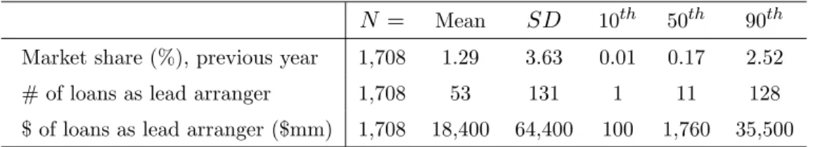
syndicated loan facilities in our sample. Panel A of Table 1 reports lead arranger
charac-teristics. We have 1,708 unique lead arranger-years. An average lead arranger has a market
share of 1.3% and arranges 53 loan facilities, which correspond to a total volume of $18.4
billion, during one year.
Panel B of Table 1 reports borrower characteristics. An average borrowing …rm in
our sample has sales of $3.23 billion at loan closing. Sixty-…ve percent had previously
borrowed from the syndicated loan market at least once, and the average number of previous
syndicated loans among all the borrowers is 3 loan facilities. Among borrowers whose …rm
type is known, 38% are identi…ed as private …rms, whereas 24% are public …rms without
bond ratings and 38% are public …rms with bond ratings.20 Among borrowers who have
Compustat data available, the average book value of total assets is $12.3 billion, the average
book leverage ratio is 37%, the average earnings to assets ratio is 7%, and 55% have S&P
debt ratings of which 56% have an investment-grade rating.
Panel C ofTable 1 shows characteristics of syndicated loan facilities in our sample. An
average syndicated loan facility has a size (loan amount) of $278 million and maturity of
49 months. The average interest spread on drawn funds is 224 basis points over LIBOR.
About one-third (31%) of the facilities are classi…ed as term loans. On average, there are
7 lenders in one syndicate, and the lead arrangers retains 32% of the loan.21 The most
common reason for borrowing is working capital or corporate purposes (62%), followed by
2 0
The …rm type indicated inDealScanis the most current status for the borrower at the end of the sample period and hence does not re‡ect the change between public and private, nor between rated and unrated, over time. Thus, we cross-check the …rm type withCompustat data, i.e., whether a borrower can be found
inCompustat at the time the loan was originated and whether a credit rating was available then.
2 1The share retained by the lead arranger is available for only 16,529 loan facilities (24% of the sample).
Thus, there may be some sample selection bias in spite of the fact that this is a widely used variable in the empirical literature on syndicated loans.
acquisitions (24%), re…nancing (21%), and backup lines (7%).22 Default occurred in 6% of
the loan facilities in the sample.
3.3.2 Distance Measures
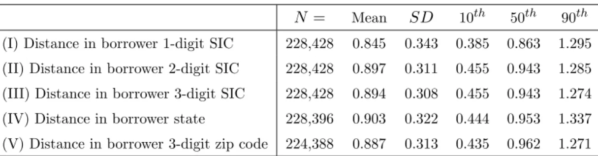
Table 2 reports summary statistics of the distance measures we described in section 2 across
the 5 specialization categories, i.e., the 1-digit, 2-digit, and 3-digit borrower SIC industry,
borrower state, and 3-digit borrower zip code . Panel AofTable 2 summarizes the distance
between any two lenders that were among the top 100 lead arrangers in each year from
1988 to 2010, whereas Panel B and Panel C of Table 2 summarizes lender distance at
the syndicated loan facility level and distance maintained by lead arrangers each year,
respectively, from 1989 to 2011. A number of important points are worth making here.
First, based on the de…nition of Euclidean distance, all distance measures must lie within
the range of 0 top2. Second, the average lender distance at the syndicated loan facility level is in the range of 0.43-0.47 and the average distance maintained by lead arrangers is in the
range of 0.63-0.70, which are both smaller than the average distance between two randomly
selected lenders (a range of 0.84-0.90). This is consistent with banks intentionally choosing
syndicate members with similar lending expertise. Third, the standard deviations of these
distance measures –0.3 for distance between two randomly selected lenders and 0.2 at the
loan as well as lead arranger level – imply that there is su¢ cient variation in the data for
empirical tests. Fourth, the distributions of distance measures across di¤erent specialization
categories are similar to one another, which indicates that our measures capture the distance
in a persistent way.
Figure 1 plots the time series of these various distance measures by year. Part A,Part
B, and Part C of Figure 1 again show distance between any two lenders, lender distance
at the loan level, and distance maintained by lead arrangers, respectively. The time-series
results indicate that in general distance has declined over time, that is, banks have become
increasingly interconnected: the most signi…cant drop occurring during 1993-1995 when
syndicated lending began to surge. There were also two small rises in lender distance
during 2001-2002 and 2007-2010. However, overall, the distance between any two randomly
selected lenders declined by 16-20% during our sample period, whereas lender distance
declined by 45-59% at the loan level and 35-45% at the lead arranger level. Interestingly,
after some increases in lender distance during the crisis period, there was another sharp
decrease in distance in the most recent year. It should be noted that given this time trend
displayed in our distance measures, we carefully control for year or loan facility …xed e¤ects
in all our empirical tests.
4
Interconnectedness of Banks in Loan Markets
In this section, we show empirically that lead arrangers tend to invite to their syndicates
lenders that are closer to themselves in terms of specialization. They are also more likely
to give lenders more senior role functions in the syndicate, i.e., co-leads and co-agents, if
these lenders have a similar specialization focus. Furthermore, the closer two lenders are
in lending expertise, the more frequently they will collaborate, and the deeper the degree
of collaboration will be. Thus, smaller distance infers stronger interconnectedness through
more collaboration. This is over and above higher exposure to common shocks, and distance
hence can be viewed as anindirect measure of interconnectedness.
We …rst examine whether banks choose close competitors, i.e. lenders with a similar
focus in lending, as syndicate partners. As outlined in the Introduction, choosing a close
competitor can have both negative e¤ects (e.g., increased competition for future business
with the same borrower) and positive e¤ects (e.g., screening and monitoring responsibilities
can be delegated to this chosen, similar lender). To understand thenet e¤ect, we estimate
the following regression:
M emberm;n;k;t= + 1dm;n;t 1+ 2 RELLm;n;t 1+ 3 RELBn;k+ 4M Sn;t 1+Fk0+ m;n;k;t,
where the dependent variableM emberm;n;k;t is an indicator variable that equals one if lead
arrangermchooses lendernas a member in loan syndicatekthat is originated in yeartand
zero otherwise. The key independent variable dm;n;t 1 measures the distance between lead
arrangerm and lendernin yeart 1. RELLm;n;t 1 is a proxy for bank-bank relationships
and measured as the number of syndicated loans lead arranger m syndicated with lender
n prior to the current loan (no matter what roles the two lenders took). RELBn;k is a
proxy for bank-…rm relationships and measured as the number of syndicated loans that
were made to the borrower prior to loan syndicate k in which lender n participated (no
matter what role it took). By including RELLm;n;t 1 and RELBn;k in the regression, we
control for the e¤ects of prior relationships between the two lenders and prior relationships
between the borrower and lender n on the construction of the syndicate, that is, who are
invited to join the syndicate. M Sn;t 1 is the market share of lender n as a lead arranger
one year before the loan was issued, i.e., yeart 1. We useM Sn;t 1 to proxy for lendern’s
reputation and market size or power. Fk is a vector of loan facility …xed e¤ects, which are
included to rule out any facility-speci…c e¤ects, including the e¤ects from the borrower, the
lead arranger, the time trend in a particular year, and any loan characteristics. Standard
errors are heteroscedasticity robust and clustered at the year level. The regression size is K
P
k=1
Mk (100 1) observations, where K is the total number of syndicated loan facilities
in the sample andMk is the number of lead arrangers in syndicatek. The resulting sample
size is nearly 11 million pairs of lenders in unique loan facilities.
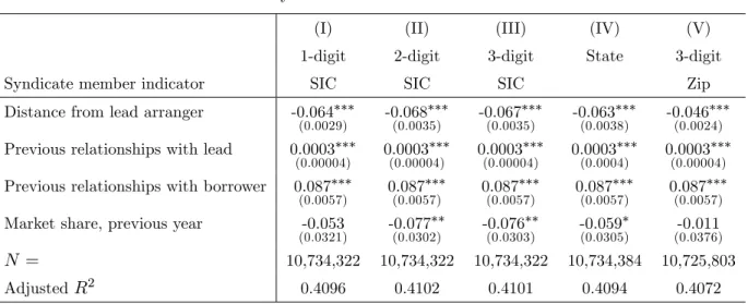
The results are reported inPanel AofTable 3. Five types of distance measures are used
in Columns (I) to (V), based on the 1-digit, 2-digit, and 3-digit borrower SIC industry,
borrower state, and the 3-digit borrower zip code, respectively. In all regressions, our
distance measures show negative coe¢ cients that are signi…cant at the 1% level. That is,
the larger the distance in lending specialization between a lender and the lead arranger,
the smaller the likelihood that the lender is chosen as a syndicate member. In other words,
the view that lead arrangers structure syndicates in order to delegate some screening and
monitoring to other syndicate members. We also …nd that a lender’s prior relationships
with either the lead arranger (RELLm;n;t 1) or the borrower (RELBn;k) have signi…cantly
positive in‡uences on the likelihood of being chosen as a syndicate member. The e¤ect is
especially strong for prior lender-borrower relationships, which con…rms the …ndings in Su…
(2007). Interestingly, lendern’s previous-year market share (M Sn;t 1) reduces its likelihood
to be included in the syndicate. This may imply a subtle balance in partner choice: banks
prefer to work with close competitors who they or the borrower worked with before and
who are not big enough to threaten future loan syndication business.23
We then analyze the e¤ect of distance on the depth of collaboration so as to seek
supporting evidence that lead arrangers collaborate to delegate screening and monitoring
responsibilities within the syndicate. We measure the depth of collaboration using the
syndicate role lenders are assigned to (typically by the lead arrangers). Based on the lender
role classi…cations described in Section 3.2, we generate a discrete variable,Rolem;n;k;t, that
takes the value 0 if lendernis not a member of the syndicate, 1 if it is a participant, 2 if it
is a co-agent, and 3 if it is a co-lead. While pure participants only contribute capital to the
syndicate, more senior roles such as co-leads and co-agents often have managerial functions
within the syndicate. A higher number for Rolem;n;k;t can therefore be associated with a
greater depth of collaboration. To test this, we estimate the following regression model:
Rolem;n;k;t = + 1 dm;n;t 1+ 2 RELLm;n;t 1+ 3 RELBn;k+ 4 M Sn;t 1+Fk0+ m;n;k;t.
(5)
The results are reported in Panel B of Table 3. We …nd a signi…cantly negative
rela-tionship between distance and syndicated role depth at the 1% level. That is, the greater
the distance from the lead arranger in terms of lending specialization, the smaller the
like-2 3
As a robustness check, we use probit and logit speci…cations with the same independent variables except loan facility …xed e¤ects and …nd the same distance e¤ect. A large number of …xed e¤ects are inappropriate for probit and logit speci…cations due to concerns of the "incidental parameters problem" [e.g., Green (2004)]. The probit and logit results are available from the authors on request.
lihood that a lender will be chosen as a senior member of the syndicate, consistent with the
view that lead arrangers structure their syndicates to delegate screening and monitoring
responsibilities to members with a similar focus and expertise in lending.24
We provide more evidence as to the importance of common lending expertise in Table
4, aggregating participation and syndicated role depth for each pair of lenders on a yearly
basis. We …nd that the frequency and depth of lender relationships decreases in distance.
In other words, collaboration is more frequent and deeper among lenders that are more
similar in lending specializations.
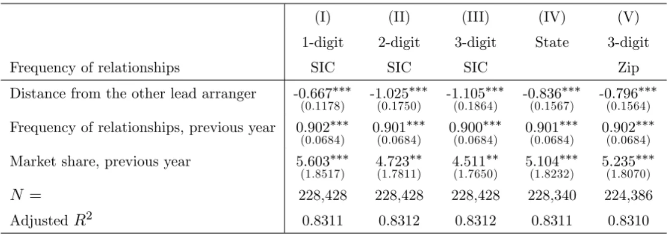
Speci…cally, Panel A ofTable 4 estimates the following regression:
F reqm;n;t= + 1 dm;n;t 1+ 2 F reqm;n;t 1+ 3 M Sn;t 1+L0m+Yt0+ m;n;t, (6)
whereF reqm;n;tis the number of times that lead arrangermchooses lendernin syndicates
it leads in year t (no matter what role lender n took) and dm;n;t 1 measures the distance
between lead arrangermand lendernin yeart 1, which is our key independent variable of
interest. F reqm;n;t 1 is the lagged value of F reqm;n;t, included in the regression to control
for the relationships between lenders m and n in the previous year so that their current
collaboration is not a simple continuation of their prior relationships. M Sn;t 1 is lendern’s
previous-year market share as a lead arranger. Lm is a vector of lead arranger …xed e¤ects
andYtis a vector of year …xed e¤ects. Note that prior lender-borrower relationships cannot
be controlled for in this regression as banks may collaborate on lending to more than one
borrower and the collaboration frequency variable is not borrower-speci…c. Regression (6)
includes approximately100 (100 1) T observations, whereT is the number of years in
the sample. The resulting sample size is close to 220,000 pairs of lenders over the sample
period of 1989-2011. The coe¢ cients on our distance measures across all …ve specialization
categories are consistently negative and signi…cant at the 1% level. That is, the closer
2 4As a robustness check, we …nd similar evidence based on ordered probit and logit speci…cations, again
two lenders are in terms of their lending specializations, the more frequently they work
together in loan syndication. In addition, the coe¢ cients on F reqm;n;t 1 and M Sn;t 1 are
signi…cantly positive, which indicates a positive impact from these two variables on lender
collaboration.
Panel B of Table 4 estimates a similar regression with the dependent variable now
measuring the aggregate depth of relationships between two banks:
Depthm;n;t= + 1 dm;n;t 1+ 2 Depthm;n;t 1+ 3 M Sn;t 1+L0m+Yt0+ m;n;t, (7)
where Depthm;n;t is the depth of all the relationships between lead arrangerm and lender
n in year t, computed as the sum of the ordinal variable, Rolem;n;k;t, for all the loans
originated by lead arranger m. That is, Depthm;n;t= KPm;t
km=1
Rolem;n;km;t, where Km;t is the
number of loans originated by lead arrangermduring yeart. Recall that Rolem;n;k;t equals
0 if lendernis not a member of the syndicatekm arranged bym, 1 if it is a participant, 2 if
it is a co-agent, and 3 if it is a co-lead. We regress the depth of relationships between lead
arranger m and lendern on their lagged distance as well as the previous-year relationship
depth between them (Depthm;n;t 1) and lender n’s previous-year market share as a lead
arranger (M Sn;t 1). Lead arranger and year …xed e¤ects are also included in regression (7).
All coe¢ cients on our distance measures are signi…cantly negative at the 5% level or better.
That is, the closer two lenders are with respect to their lending expertise, the deeper their
collaboration in the syndicated loan market. In addition, the coe¢ cients on Depthm;n;t 1
and M Sn;t 1 are again signi…cantly positive as expected.
One possible argument is that our distance e¤ect is driven by the size of large banks.
Large banks typically invest in more industries and/or locations, that is, they are more
diversi…ed with regards to their loan portfolios. Consequently, on average the distance
between two large banks will be smaller than the distance between two smaller banks or the
distance between one large bank and one small bank. Thus, since large banks frequently
e¤ects of bank size rather than thetrue organizational form of loan syndicates. To examine
this, we control for bank size by including each bank’s syndicated loan market share in the
regressions speci…ed above. In addition, to further show that bank size is not a concern,
we exclude the top three to ten lead arrangers of each sample year from all regressions and
obtain qualitatively similar results.25 In other words, distance is an important factor when
banks choose partners, regardless of the bank size.
Taken together, we …nd a propensity of bank lenders to concentrate syndicate partners
rather than to diversify them. In the next section, we provide evidence as to the bene…ts
of this strategy.
5
E¢ ciency Gains in Screening and Monitoring
Section 4 provides important insights into how banks choose partners in loan syndicates.
The question still arises as to why the organizational structure matters. To address this
question, we examine in this section what di¤erent strategies mean to borrowers and lenders.
5.1 Close versus Distant Syndicates
A possible bene…t of inviting similar lenders in syndicates is e¢ ciency gains, for example,
with respect to screening and monitoring [Strausz (1997)]. To explore this, we …rst use the
lender distance at the loan facility level [as de…ned in Equation (2)] to group our sample
of syndicated loans into close and distant syndicates. The sub-sample of close syndicates
consists of syndicates in which lender distance is below the median lender distance in the
originating year, whereas the sub-sample of distant syndicates consists of the remaining
syn-dicates, i.e., those with lender distance above the median. We then look into the di¤erences
between close and distant syndicates.26
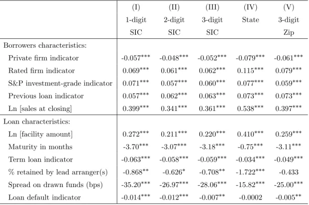
Table 5 reports the mean di¤erences for key borrower and loan characteristics between
the two sub-samples, i.e., Close– Distant. We …nd that on average borrowers of close
syn-2 5Results are available from the authors on request. 2 6
dicates are less likely to be private …rms but more likely to be rated, have S&P
investment-grade ratings, have borrowed previously from the syndicated loan market, and show higher
sales at loan closing. In addition, close syndicates tend to have larger loan size, shorter
ma-turity, and fewer term loans. In other words, close syndicates seem to have safer borrowers
and safer loans. All these di¤erences are statistically signi…cant at the 1% level.
Furthermore, the average loan share retained by lead arrangers is about 0.4-1.7% lower
among close syndicates. The di¤erences are signi…cant at the 10% level or better across all
…ve specialization categories except the 3-digit borrower zip code. With respects to loan
pricing and loan default rates, we …nd that close syndicates: (1) o¤er on average lower
interest spreads on drawn funds over LIBOR by 15-35 basis points and (ii) result in a lower
default rate of 0.5-1.4% in all cases except measured by borrower state. These di¤erences
are signi…cant at the 5% level or better. Such results from bivariate tests are in general
consistent with e¢ ciency gains from screening and monitoring.
In Sections 5.2-5.4 below we examine the e¤ect of distance on syndicate structure, loan
pricing, and loan default in a more formal regression framework.
5.2 Distance and Syndicate Structure
If lead arrangers choose their syndicate partners to delegate some screening and monitoring
responsibilities, they must give these lenders incentives to ful…ll these tasks diligently. Such
incentives arise from the shares of a loan these lenders hold. The closer a lender is to the
lead arranger, the more likely it will be delegated responsibilities to, then the stronger the
need for incentives through a higher share of the loan. Thus, we expect that the distance
in specialization between a lead arranger and a syndicate lender is negatively related to
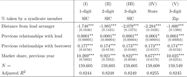
speci…cation:
Sharem;n;k;t= + 1 dm;n;t 1+ 2 RELLm;n;t 1+ 3 RELBn;k+ 4 M Sn;t 1+Fk0+ m;n;k;t,
(8)
whereSharem;n;k;tis the share of loan syndicatek held by lendern, anddm;n;t 1 measures
the distance between lead arranger mand lender nin year t 1. RELLm;n;t 1,RELBn;k,
M Sn;t 1, andFkare the same as de…ned in Equations (4) and (5) above. That is, we regress
loan share taken by lendern in syndicatekon its lagged distance from lead arranger mas
well as control variables such as lendern’s prior relationships with lead arranger mand the
borrower, lender n’s previous-year market share as a lead arranger itself, and loan facility
…xed e¤ects. This regression includes close to 160,000 pairs of syndicate lenders on unique
loan facilities. Note that the e¤ect of distance on Sharem;n;k;t in Equation (8) is estimated
conditional on the fact that lender n is a member lender of the syndicate, i.e., was chosen
by the lead arranger. Based on our results in Section 4, this group of lenders are relatively
closer to the lead arranger compared to those who were not selected at all. Thus, variation
in distance among this particular group is smaller compared to the whole sample.
Table 6 shows results for our distance measures across …ve specialization categories.
Having controlled for prior relationships (i.e., RELLm;n;t 1 and RELBn;k,) and lender
size/reputation (i.e., M Sn;t 1), we …nd that the coe¢ cients on our distance measures are
consistently negative and signi…cant at the 1% level. These results are consistent with
syndicate lenders holding signi…cantly larger loan shares if they have similar lending
spe-cializations as the lead arranger, i.e., distance is smaller. We also …nd that a lender’s loan
share more signi…cantly increases with its prior relationship with the borrower than with
the lead arranger. In addition, a lender’s market share has a signi…cantly positive impact
on its loan share, which may be related to larger players in the market having more funds
5.3 Distance and Loan Pricing
There exist potentially two possible e¤ects of pricing from lender distance. First, borrowers
might bene…t from smaller lender distance because lead arrangers can pass on some savings
from screening and monitoring costs to borrowers. However, collaboration among close
competitors might also lead to extraction of rents (higher spreads) from borrowers. Our
bivariate tests show that close loan syndicates are associated with lower spreads, suggesting
that borrowers can internalize some of the e¢ ciency gains. To examine the net e¤ect of
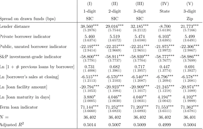
distance on loan pricing more formally, we run the following regression:
Spreadk;l;s;t= + 1 Dk;t+ 2L0l;t+ 3Mk0 +Is0 +Yt0+ k;l;s;t, (9)
whereSpreadk;l;s;t is the interest spread over LIBOR on drawn funds. As de…ned in
Equa-tion (2),Dk;t is the lender distance in syndicated loankissued to borrowerl. Ll;tis a vector
of borrower control variables as of year t, including whether borrower l is a private …rm,
whether it has a publicly available rating, whether it has an S&P investment-grade rating,
the number of syndicated loan previously borrowed, and sales at closing. Mk is a vector
of loan control variables, including loan amount, maturity, whether it is a term loan, loan
purpose, and interest rate type (i.e., …xed vs. ‡oating). Isis a vector of borrower two-digit
SIC industry …xed e¤ects andYtis a vector of year …xed e¤ects. The unit of observation is
a loan facility.
The results are reported in Table 7. Our distance measures are all positive and
sig-ni…cant at the 1% level except distance based on borrower state. Thus, on a net basis,
borrowers actually bene…t from working with close loan syndicates by paying lower loan
spreads. The saving is 7-13 basis points for a reduction of one standard deviation in lender
distance based on borrower industry and zip code. This result is consistent with lenders
sharing some bene…ts from low lender distance with their borrowers. In addition, coe¢
and increase in maturity, (ii) loans are cheaper for borrowers with S&P investment-grade
ratings as well as higher sales, and (iii) term loans pay higher spreads of about 71 basis
points on average.
Taken together, these results are consistent with the view that close syndicate members
can help with screening and monitoring so as to reduce the overall loan syndication costs.
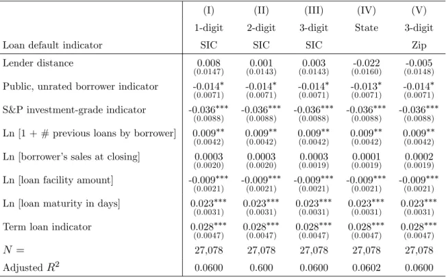
5.4 Distance and Loan Default
We next examine whether potential e¢ ciency gains from constructing close syndicates
ex-tend to lower default rates. We estimate the following regression:
Def aultk;l;s;t= + 1 Dk;t+ 2L0l;t+ 3Mk0 +Is0 +Yt0+ k;l;s;t, (10)
where Def aultk;l;s;t is an indicator variable that equals one if the loan is in default and
zero otherwise. Ll;t,Mk,Is andYtare the same control variables and …xed e¤ects as in the
regression of loan interest spread [i.e., Equation (9)]. That is, we regress loan default on
lender distance, loan and borrower characteristics, and industry and year …xed e¤ects. Since
the independent variables include whether the borrower is rated, whether its rating is of an
investment grade, and its sales at loan closing, we control forex-ante borrower quality and
creditworthiness and hence the coe¢ cient on lender distance indicates the e¤ect of distance
on subsequent loan default. The regression is estimated at the loan facility level. Table 8
reports the regression results from a linear probability model. We …nd no evidence that
closer distance reduces loan default rates.27
6
Interconnectedness and Systemic Risk
The previous sections demonstrate that the syndication process has made the loan portfolios
of banks increasingly similar over the last two decades. In other words, it increased the
2 7As a robustness check, we use probit and logit speci…cations with the same independent variables and
interconnectedness of banks that were active in the loan syndicate network. While there
are bene…ts to syndication (some of which we have analyzed earlier in this paper), it also
creates systemic risk because problems of some banks can spread throughout this network
for di¤erent reasons: banks are exposed to each other, exposed to similar assets, and exposed
to the same type of investors who eventually run on some banks because of problems that
surfaced at other banks (and the inherent opaqueness of the banking sector).
In our empirical analysis, we follow the de…nition of systemic risk as outlined in Acharya
et al. (2010) as the contribution of each individual bank to the aggregate capital shortfall
during a systemic crisis when there is an aggregate shortage of capital in the …nancial
sector. Systemic risk occurs if the …nancial sector is undercapitalized because the reduction
in lending by one institution cannot be o¤set by other …nancial institutions and might
cause a credit crunch. Acharya et al. (2010) measure systemic risk as the amount by
which a bank is undercapitalized in a systemic event in which the entire …nancial system is
undercapitalized, and they term it the systemic expected shortfall or SES. This concept
is appealing as it uses market data that are readily available to regulators and market
participants. They show that SES is the bank’s level of undercapitalization assuming a
target leverage ratio (for example, 8%). They demonstrate that SES can be explained
by two factors. The …rst is theex-ante market-leverage ratio of the bank, and the second
captures the downside exposure to systemic shocks which they call the marginal expected
shortfall (M ES). M ES is the expected equity loss of one bank when the market declines
beyond a speci…c threshold over a given period. Acharya et al. (2010) and Brownlees and
Engle (2010) develop a systemic risk indexSRISK%i which is the capital shortfall of one
bank relative to the …nancial sector. The concept is very intuitive. Suppose that k is the
prudential capital ratio, say 8%, Di;1 is …rm’s i debt in period 1, and Wi;1 (Wi;2) is the
is then
CSi;1 = E1[k(Di;1+Wi;2) Wi;2jCrisis] (11)
= kDi;1 (1 k)Wi;1M ESi;1
The …rm experiences a capital shortfall only if CSi;1>0, i.e.
SRISKi;1 = min(0; CSi;1) (12) SRISK%i;1 = SRISKi;1 X i SRISKi;1
whereSRISK%is the percentage version. M ESis measured dynamically using asymmetric
GARCH models and DCC.
NYU’s Volatility Laboratory (V-Lab) Global Systemic Risk Database ("SRISK")
pro-vides systemic risk measures for about 1,200 publicly traded …nancial institutions worldwide.
We can match 53 of our top 100 lead arrangers to SRISK.Appendix 3 shows a list of these
institutions. Interestingly, 24 of these institutions are also part of the FSB’s list of
Global-SIFIs which more stresses the interconnectedness of the global …nancial institutions even in
the U.S. syndicated loan market.28
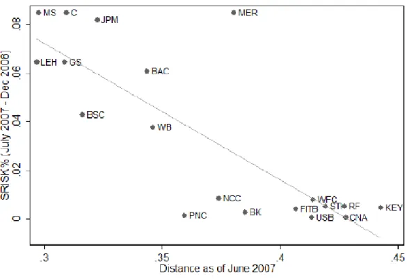
We start analyzing the impact of interconnectedness on systemic risk graphically using
the top lead arrangers as of June 2007. Forty international institutions were responsible
for 96% of the syndicated loan origination as of that date. Twenty-two of them were U.S.
…rms, among which were Wachovia, Lehman Brothers, and Bear Sterns. All three belonged
to the top 15 originators that year.
We analyze whether the distance maintained by a bank [as de…ned in Equation (3)] can
predict its contribution to the capital shortfall of the …nancial sector during a systemic crisis.
We collect monthly SRISK%i measures from SRISK and calculate an average relative
shortfall measure for each bank during the period from July 2007 to December 2008. We
2 8
plot this measure against our distance measure in Figure 2, of which Part A shows U.S.
…nancial institutions, Part B shows European institutions, and Part C includes the full
sample. We …nd that distance explains a major part of the variation of SRISK%i (R2 is
above 50%). As distance is our measure of interconnectedness, this is equivalent to say that
the most interconnected banks are also the greatest contributors to systemic risk.
In a next step, we test this interconnectedness-systemic risk relation in a multivariate
setting using monthlySRISK%data for the period from January 2000 to November 2011.
As not all …rms survived the …nancial crisis or had publicly traded equity throughout this
time period, the panel is unbalanced with 4,998 bank-month observations. Our
depen-dent variable is Ln [SRISK%] which is the natural logarithm ofSRISK%to account for
the skewness of the variable. SRISK% is left censored at 0 and our sample has 1,506
left-censored observations. That is,Ln[SRISK%] is available for 3,492 bank-month
obser-vations.29 We construct an indicator variable European which equals 1 if the institution
is headquartered in Europe. To account for di¤erences between Europe and the U.S. we
introduce the interaction termDistance European. We also include as control variables
(i) the natural logarithm of the quasi-market leverage ratio which is calculated as book total
assets minus book value of equity plus market value of equity, scaled by market value of
equity, and (ii) the natural logarithm of market value of equity. Both leverage and market
value of equity come from SRISK. All regressions further include year-quarter …xed e¤ects.
We assess the e¤ect of Distance onLn [SRISK%] using OLS regressions. The results are
reported inTable 9.
Model (I) of Table 9 shows that more interconnected lenders contribute more to
sys-temic risk. The e¤ect is signi…cant at the 1% level and the R2 is 15.94%. In Models (II)
and (III), we introduce European and Distance European. European …nancial
insti-tutions have a higher systemic risk index. We control for leverage in Model (IV). As we
are interested in the change in the contribution to systemic risk of one bank relative to
2 9We perform additional robustness tests using SRISK% as dependent variable and tobit regressions
the other banks if interconnectedness changes, we estimate a between e¤ects model. The
results are reported in Model (V) of Table 9. The nature of the coe¢ cient on our distance
measure is unchanged. We then includeLn[market value]as control for bank size in
Mod-els (VI) and (VII). Due to high correlation betweenEuropeanand Ln[market value], we
exclude European and its interaction term with distance in these two models. The results
for distance, however, remain unchanged. We test di¤erent model speci…cations introducing
interaction terms betweenEuropean,Ln[leverage]and Ln [market value]to account for
the elevated correlation without any e¤ect on our results. We omit these tests for brevity.
Taken together, we …nd strong supporting evidence to our conjecture that the most
interconnected banks are also the greatest contributor to systemic risk.
7
Conclusion
This paper studies interconnectedness of banks in the syndicated loan market as a major
source of systemic risk. We develop a set of novel measures to describe how banks are
interconnected based on the similarity of their loan portfolios. We use a dataset of newly
originated syndicated loans for the period from 1988 to July 2011 and analyze which banks
are invited to join the syndicates and how this is in‡uenced by their existing loan portfolios.
We …nd a propensity of banks to concentrate syndicate lenders rather than to diversify them.
We analyze potential bene…ts of this behavior and …nd evidence consistent with the view
that close syndicate members can help with screening and monitoring so as to reduce the
overall loan syndication costs. More speci…cally, we …nd that lead arrangers assign more
responsibilities to banks they are already connected with and have these banks take on
higher shares of the loan as incentive. We also …nd signi…cantly lower loan spreads for
closer syndicates, which suggest that cost savings exist and borrowers can internalize a
fraction of these savings.
Subsequently and more importantly, we analyze potential negative externalities
market, we …nd that interconnectedness of banks can explain the downside exposure of
these banks to systemic shocks. Moreover, we …nd that the most interconnected banks are
also the greatest contributors to systemic risk.
References
[1] Acharya, Viral V., Lasse Pedersen, Thomas Philippon and Matthew Richardson (2010),
Measuring Systemic Risk, Working Paper, NYU Stern.
[2] Adrian, Tobias, and Markus K. Brunnermeier (2008), CoVaR, Fed Reserve Bank of
New York Sta¤ Reports.
[3] Allen, Franklin and Ana Babus, 2008, Networks in Finance, The Network Challenge:
Strategy, Pro…t, and Risk in an Interlinked World (Paul R. Kleindorfer, Yoram Wind,
and Robert E. Gunther, eds.), Wharton School Publishing.
[4] Allen, Linda, Turan Bali, and Yi Tang (2010), Does Systemic Risk in the Financial
Sector Predict Future Economic Downturns?, Baruch College Working Paper.
[5] Allen, Franklin and Douglas Gale, 2000, Financial Contagion, Journal of Political
Economy, Vol. 108, No. 1, 1-33.
[6] Bharath, Sreedhar T., Sandeep Dahiya, Anthony Saunders and Anand Srinivasan,
2011, Lending Relationships and Loan Contract Terms, Review of Financial Studies,
Vol. 24, No. 5, 1141-1203.
[7] Billio, Monica, Mila Getmansky, Andrew Lo, and Loriana Pelizzon (2010), Econometric
Measures of Systemic Risk in the Finance and Insurance Sectors, NBER Paper No.
16223.
[8] Brownlees, Christian and Robert Engle (2010), Volatility, Correlation and Tails for
[9] Brunnermeier, Markus K., Gang Dong, and Darius Palia (2011), Banks’Non-Interest
Income and Systemic Risk, Working Paper.
[10] Cai, Jian, 2009, Competition or Collaboration? The Reciprocity E¤ect in Loan
Syn-dication, Working Paper.
[11] Chan-Lau, Jorge (2010), Regulatory Capital Charges for Too-Connected-to-Fail
Insti-tutions: A Practical Proposal, IMF Working Paper 10/98
[12] Chowdhry, Bhagwan and Vikram Nanda, 1996, Stabilization, Syndication and Pricing
of IPOs, Journal of Financial and Quantitative Analysis, Vol. 31, No. 1, 25-42.
[13] Cohen, Lauren, Andrea Frazzini and Christopher Malloy, 2007, The Small World of
Investing: Board Connections and Mutual Fund Returns, NBER Working Paper No.
13121.
[14] Dennis, Steven A. and Donald J. Mullineaux, 2000, Syndicated Loans, Journal of
Financial Intermediation, 9, 404-426.
[15] Diamond, Douglas W., 1984, Financial Intermediation and Delegated Monitoring,
Re-view of Economic Studies, Vol. 51, No. 3, 393-414.
[16] François, Pascal and Franck Missonier-Piera, 2007, The Agency Structure of Loan
Syndicates, Financial Review, 42, 227-245.
[17] Freixas, Xavier, Bruno M. Parigi and Jean-Charles Rochet, 2000, Systemic Risk,
In-terbank Relations, and Liquidity Provision by the Central Bank, Journal of Money,
Credit and Banking, Vol. 32, No. 3, 611-638.
[18] Gatev, Evan and Philip E. Strahan, 2009, Liquidity Risk and Syndicate Structure,
Journal of Financial Economics, Vol. 93, No. 3, 490-504.
[19] Giannetti, Mariassunta and Yishay Yafeh, 2009, Do Cultural Di¤erences Between
[20] Gopalan, Radhakrishnan, Vikram Nanda and Vijay Yerramilli, 2011, Does poor
per-formance damage the reputation of …nancial intermediaries? Evidence from the loan
syndication market, Journal of Finance, Vol. 66, No. 6, 2083-2120.
[21] Goyal, Sanjeev and José Luis Moraga-González, 2001, R&D Networks, Rand Journal
of Economics, Vol. 32, No. 4, 686-707.
[22] Goyal, Sanjeev, José Luis Moraga-González and Alexander Konovalov, 2008, Hybrid
R&D, Journal of the European Economic Association, Vol. 6, No. 6, 1309-1338.
[23] Greene, William, 2004, Fixed E¤ects and Bias Due to the Incidental Parameters
Prob-lem in the Tobit Model, Econometric Reviews, Vol. 23, No. 2, 125-147.
[24] Gupta, Anurag, Ajai K. Singh and Allan A. Zebedee, 2008, Liquidity in the Pricing of
Syndicated Loans, Journal of Financial Markets, Vol. 11, No. 4, 339-376.
[25] Hochberg, Yael V., Alexander Ljungqvist and Yang Lu, 2007, Whom You Know
Mat-ters: Venture Capital Networks and Investment Performance, Journal of Finance, Vol.
LXII, No. 1, 251-301.
[26] Holmstrom, Bengt, 1982, Moral Hazard in Teams, Bell Journal of Economics 13,
324-340.
[27] Holmstrom, Bengt and Jean Tirole, 1997, Financial Intermediation, Loanable Funds,
and the Real Sector, Quarterly Journal of Economics, Vol. 112, No. 3, 663-691.
[28] Huang, Xin, Hao Zhou, and Haibin Zhu (2009), A Framework for Assessing the
Sys-temic Risk of Major Financial Institutions, Journal of Banking and Finance 33,
2036-2049.
[29] Ivashina, Victoria, 2009, Asymmetric Information E¤ects on Loan Spreads, Journal of