Rectifying Classifier Chains for
Multi-Label Classification
Robin Senge
1, Juan Jos´e del Coz
2and Eyke H ¨ullermeier
11
:Department of Mathematics and Computer Science, University of Marburg, Germany
2:Artificial Intelligence Center, University of Oviedo at Gij´on, Spain
Abstract
Classifier chains have recently been proposed as an appealing method for tackling the multi-label classification task. In addition to several em-pirical studies showing its state-of-the-art perfor-mance, especially when being used in its ensem-ble variant, there are also some first results on theoretical properties of classifier chains. Con-tinuing along this line, we analyze the influ-ence of a potential pitfall of the learning pro-cess, namely the discrepancy between the fea-ture spaces used in training and testing: While true class labels are used as supplementary at-tributes for training the binary models along the chain, the same models need to rely on estima-tions of these labels at prediction time. We elu-cidate under which circumstances the attribute noise thus created can affect the overall predic-tion performance. As a result of our findings, we propose two modifications of classifier chains that are meant to overcome this problem. Exper-imentally, we show that our variants are indeed able to produce better results in cases where the original chaining process is likely to fail.
1
Introduction
Multi-label classification (MLC) has attracted increasing attention in the machine learning community during the past few years. Apart from being interesting theoretically, this is largely due to its practical relevance in many do-mains, including text classification, media content tagging and bioinformatics, just to mention a few. The goal in MLC is to induce a model that assigns asubsetof labels to each example, rather than a single one as in multi-class classifi-cation. For instance, in a news website, a multi-label classi-fier can automatically attach several labels—usually called tags in this context—to every article; the tags can be help-ful for searching related news or for briefly informing users about their content.
Current research on MLC is largely driven by the idea that optimal predictive performance can only be achieved by modeling and exploiting statistical dependencies be-tween labels. Roughly speaking, if the relevance of one label may depend on the relevance of others, then labels should be predicted simultaneously and not separately. This is the main argument against simple decomposition techniquessuch as binary relevance (BR) learning, which splits the original multi-label task into several independent binary classification problems, one for each label.
Until now, several methods for capturing label depen-dence have been proposed in the literature. They can be categorized according to two major properties: (i) the size of the subsets of labels for which dependencies are modeled and (ii) the type of label dependence they seek to capture. Looking at the first property, there are methods that only consider pairwise relations between labels [5; 6; 14; 19] and approaches that take into account correlations among larger label subsets [12; 13; 17]; the latter include those that consider the influence of all labels simultaneously [2; 8; 11]. Regarding the second criterion, it has been proposed to distinguish between the modeling ofconditionaland un-conditional label dependence[3; 4], depending on whether the dependence is conditioned on an instance [3; 11; 13; 16] or describing a kind of global correlation in the label space [2; 8; 19].
In this paper, we focus on a method called classifier chains (CC) [13]. This method enjoys great popularity, even though it has been introduced only lately. As its name suggests, CC selects an order on the label set—a
chainof labels—and trains a binary classifier for each la-bel in this order. The difference with respect to BR is that the feature space used to induce each classifier is ex-tended by the previous labels in the chain. These labels are treated as additional attributes, with the goal to model con-ditional dependence between a label and its predecessors. CC performs particularly well when being used in an en-semble framework, usually denoted asensemble of classi-fier chains(ECC), which reduces the influence of the label order.
Our study aims at gaining a deeper understanding of CC’s learning process. More specifically, we address an issue that, despite having been noticed [4], has not been picked out as an important theme so far: Since informa-tion about preceding labels is only available for training, this information has to be replaced by estimations (com-ing from the correspond(com-ing classifiers) at prediction time. As a result, CC has to deal with a specific type of attribute noise: While a classifier is learnt on “clean” training data, including the true values of preceding labels, it is applied on “noisy” test data, in which true labels are replaced by possibly incorrect predictions. Obviously, this type of noise may affect the performance of each classifier in the chain. More importantly, since each classifier relies on its prede-cessors, a single false prediction might be propagated and possibly even reinforced along the whole chain.
The contribution of this paper is twofold. First, we ana-lyze the above problem of classifier chains in more detail. Using both synthetic and real data sets, we design exper-iments in order to reveal those factors that influence the effect of error propagation in CC. Second, we propose and
evaluate modifications of the original CC method that are intended to overcome this problem.
The rest of the paper is organized as follows. The next section introduces the setting of MLC more formally, and Section 3 explains the classifier chains method. Section 4 is devoted to a deeper discussion of the aforementioned pit-falls of CC, along with some first experiments for illustra-tion purposes.1 In Section 5, we introduce modifications of CC and propose a method callednested stacking. An empirical study, in which we experimentally compare this method with the original CC approach, is presented in Sec-tion 6. The paper ends with a couple of concluding remarks in Section 7.
2
Multi-Label Classification
LetL = {λ1, λ2, . . . , λm}be a finite and non-empty set
of class labels, and letX be an instance space. We con-sider a MLC task with a training setS = {(x1,y1), . . . ,
(xn,yn)}, generated independently according to a
prob-ability distributionP(X,Y) onX × Y. Here, Y is the set of possible label combinations, i.e., the power set of
L. To ease notation, we define yi as a binary vector
yi = (yi,1, yi,2, . . . , yi,m), in whichyi,j = 1indicates the
presence (relevance) andyi,j= 0the absence (irrelevance)
ofλjin the labeling ofxi. Under this convention, the
out-put space is given byY = {0,1}m. The goal in MLC is
to induce fromSa hypothesish:X −→ Ythat correctly predicts the subset of relevant labels for unlabeled query instancesx.
The most straightforward and arguably simplest ap-proach to tackle the MLC problem isbinary relevance(BR) learning. The BR method reduces a given multi-label prob-lem with m labels to m binary classification problems. More precisely,mhypothesesh1, h2, . . . , hmare induced,
each of them being responsible for predicting the relevance of one label, usingX as an input space:
hj:X −→ {0,1} (1)
In this way, the labels are predicted independently of each other and no label dependencies are taken into account.
In spite of its simplicity and the strong assumption of la-bel independence, it has been shown theoretically and em-pirically that BR performs quite strong in terms of decom-posable loss functions [3], including the well-known Ham-ming loss: LH(y,h(x)) = 1 m m X i=1 [[yi6=hi(x)]] (2)
The Hamming loss averages the standard 0/1 classification error over themlabels and hence corresponds to the pro-portion of labels whose relevance is incorrectly predicted. Thus, if one of the labels is predicted incorrectly, this ac-counts for an error ofm1. Another extension of the standard 0/1 classification loss is thesubset 0/1 loss:
LZO(y,h(x)) = [[y6=h(x)]] (3)
Obviously, this measure is more drastic and already treats a mistake on a single label as a complete failure. The ne-cessity to exploit label dependencies in order to minimize the generalization error in terms of the subset 0/1 loss has been shown in [3].
1
This section is partly based on [15]
3
Classifier Chains
While following a similar setup as BR, classifier chains (CC) seek to capture label dependencies. CC learns m
binary classifiers linked along a chain, where each classi-fier deals with the binary relevance problem associated with one label. In the training phase, the feature space of each classifier in the chain is extended with the actual label in-formation of all previous labels in the chain. For instance, if the chain follows the orderλ1→λ2→. . .→λm, then
the classifierhjresponsible for predicting the relevance of
λjis of the form
hj : X × {0,1}j−1−→ {0,1} . (4)
The training data for this classifier consists of instances
(xi, yi,1, . . . , yi,j−1) labeled with yi,j, that is, original
training instancesxisupplemented by the relevance of the
labelsλ1, . . . , λj−1precedingλjin the chain.
At prediction time, when a new instancexneeds to be la-beled, a label subsety= (y1, . . . , ym)is produced by
suc-cessively querying each classifierhj. Note, however, that
the inputs of these classifiers are not well-defined, since the supplementary attributesyi,1, . . . , yi,j−1are not avail-able. These missing values are therefore replaced by their respective predictions:y1used byh2as an additional input is replaced byyˆ1 =h1(x),y2used byh3as an additional input is replaced byyˆ2 = h2(x,yˆ1), and so forth. Thus, the predictionyis of the form
y= h1(x), h2(x, h1(x)), . . .
Realizing that the order of labels in the chain may influence the performance of the classifier, and that an optimal order is hard to anticipate, the authors in [13] propose the use of an ensemble of CC classifiers. This approach combines the predictions of different random orders and, moreover, uses a different sample of the training data to train each member of the ensemble.Ensembles of classifier chains(ECC) have been shown to increase predictive performance over CC by effectively using a simple voting scheme to aggregate pre-dicted relevance sets of the individual CCs: For each label
λj, the proportionwˆj of classifiers predictingyj = 1is
calculated. Relevance of λj is then predicted by using a
thresholdt, that is,yˆj = [[ ˆwj≥t]].
4
The Problem of Attribute Noise in
Classifier Chains
The learning process of CC violates a key assumption of supervised learning, namely the assumption that the train-ing data is representative of the test data in the sense of be-ing identically distributed. This assumption does not hold for the chained classifiers in CC: While using thetruelabel datayjas input attributes during the training phase, this
in-formation is replaced byestimationsyˆjat prediction time.
Needless to say, yj andyˆj are not guaranteed to follow
the same distribution; on the contrary, unless the classifiers produce perfect predictions, these distributions are likely to differ in practice (in particular, note that theyˆj are
de-terministic predictions whereas the yj normally follow a
non-degenerate probability distribution).
From the point of view of the classifierhj, which uses
the labelsy1, . . . , yj−1 as additional attributes, this prob-lem can be seen as a probprob-lem of attribute noise. More specifically, we are facing the “clean training data vs. noisy test data” case, which is one of four possible noise scenar-ios that have been studied quite extensively in [20]. For CC,
this problem appears to be vital: Could it be that the addi-tional label information, which is exactly what CC seeks to exploit in order to gain in performance (compared to BR), eventually turns out to be a source of impairment? Or, stated differently, could the additional label informa-tion perhaps be harmful rather than useful?
This question is difficult to answer in general. In partic-ular, there are several factors involved, notably the follow-ing:
• The length of the chain: The larger the numberj−1 of preceding classifiers in the chain, the higher is the potential level of attribute noise for a classifierhj. For
example, if prediction errors occur independently of each other with probability, then the probability of a noise-free input is only(1−)j−1. More realistically, one may assume that the probability of a mistake is not constant but will increase with the level of attribute noise in the input. Then, due to the recursive structure of CC, the probability of a mistake will be reinforced and increase even more rapidly along the chain.
• The order of the chain: Since some labels might be inherently more difficult to predict than others, the or-der of the chain will play a role, too. In particular, it would be advantageous to put simpler labels in the beginning and harder ones more toward the end of the chain.
• The accuracy of the binary classifiers: The level of attribute noise is in direct correspondence with the ac-curacy of the binary classifiers along the chain. More specifically, these classifiers determine the input dis-tributions in the test phase. If they are perfect, then the training distribution equals the test distribution, and there is no problem. Otherwise, however, the distribu-tions will differ.
• The dependency among labels: Perhaps most interest-ingly, a (strong enough) dependence between labels is a prerequisite for both, an improvement and a de-terioration through chaining. In fact, CC cannot gain (compared to BR) in case of no label dependency. In that case, however, it is also unlikely to loose, because a classifierhj will most likely2 ignore the attributes
y1, . . . , yj−1. Otherwise, in case of pronounced
la-bel dependence, it will rely on these attributes, and whether or not this is advantageous will depend on the other factors above.
In the following, we present two experimental studies that are meant to illustrate the above issues. Based on our dis-cussion so far and these experiments, two modifications of CC will then be introduced in the next sections, both of them with the aim to alleviate the problems outlined above.
4.1
First Experiment
Our intuition is that attribute noise in the test phase can produce a propagation of errors through the chain, thereby affecting the performance of the classifiers depending on their position in the chain. More specifically, we expect classifiers in the beginning of the chain to systematically perform better than classifiers toward the end. In order to verify this conjecture, we perform the following simple ex-periment: We train a CC classifier on 500 randomly gen-erated label orders. Then, for each label order and each
2
The possibility to ignore parts of the input information does of course also depend on the type of base classifier used.
2 4 6 8 10 0.00 0.04 0.08 0.12 label position po si tio n-w ise re la tive in cre ase o f cl assi fica tio n erro r BR - all CC - emotions CC - scene CC - yeast-10
Figure 1: Results of the first experiment: position-wise rel-ative increase of classification error (mean plus standard error bars). Theyeast-10data set used here is a reduced yeast data set containing only the ten most frequent labels and their instances.
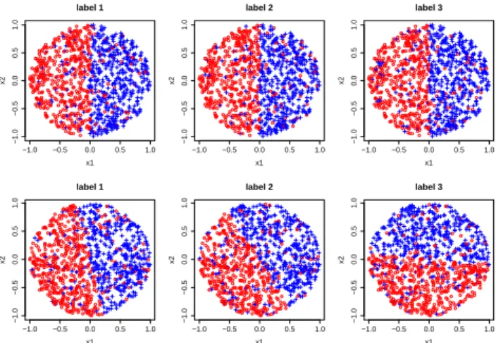
−1.0 −0.5 0.0 0.5 1.0 −1.0 −0.5 0.0 0.5 1.0 label 1 x1 x2 −1.0 −0.5 0.0 0.5 1.0 −1.0 −0.5 0.0 0.5 1.0 label 2 x1 x2 −1.0 −0.5 0.0 0.5 1.0 −1.0 −0.5 0.0 0.5 1.0 label 3 x1 x2 −1.0 −0.5 0.0 0.5 1.0 −1.0 −0.5 0.0 0.5 1.0 label 1 x1 x2 −1.0 −0.5 0.0 0.5 1.0 −1.0 −0.5 0.0 0.5 1.0 label 2 x1 x2 −1.0 −0.5 0.0 0.5 1.0 −1.0 −0.5 0.0 0.5 1.0 label 3 x1 x2
Figure 2: Example of synthetic data: the top three labels are generated usingτ = 0, the three at the bottom with
τ= 1.
position, we compute the performance of the classifier on that position in terms of the relative increase of classifica-tion error compared to BR. Finally, these errors are aver-aged position-wise(not label-wise). For this experiment, we used three standard MLC benchmark data sets whose properties are summarized in Table 1 (shown in Section 5). The results in Figure 1 clearly confirm our expectations. In two cases, CC starts to loose immediately, and the loss increases with the position. In the third case, CC is able to gain on the first positions but starts to loose again later on.
4.2
Second Experiment
In a second experiment, we use a synthetic setup that was proposed in [4] to analyze the influence of label depen-dence. The input spaceX is two-dimensional and the un-derlying decision boundary for each label is linear in these inputs. More precisely, the model for each label is defined as follows:
hj(x) =
1 aj,1x1+aj,2x2≥0
0 otherwise (5)
The input values are drawn randomly from the unit circle. The parametersaj,1andaj,2for thej-th label are set to
5 10 15 20 25
1.05
1.10
1.15
1.20
tau = 0 (high label dependence)
number of labels (subset 0/1 loss) / Ba y es 5 10 15 20 25 1.45 1.55 1.65
tau = 0 (high label dependence)
number of labels (Hamming loss) / Ba y es BR CC ECC 5 10 15 20 25 1.05 1.15 1.25 1.35
tau = 1 (low label dependence)
number of labels (subset 0/1 loss) / Ba y es 5 10 15 20 25 1.5 1.6 1.7 1.8 1.9 2.0
tau = 1 (low label dependence)
number of labels
(Hamming loss) / Ba
y
es
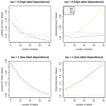
Figure 3: Results of the second experiment for τ = 0 (top—high label dependence) andτ = 1(bottom—low la-bel dependence).
withr1andr2randomly chosen from the unit interval. Ad-ditionally, random noise is introduced for each label by in-dependently reversing a label with probability π = 0.1. Obviously, the level of label dependence can be controlled by the parameterτ. Figure 2 shows two example data sets with three labels. The first one (pictures on the top) is gen-erated withτ = 0, the second one (bottom) withτ = 1. As can be seen, the label dependence is quite strong in the first case, where the model parameters (6) are the same for each label. For the second case, the model parameters are different for each label. There is still label dependence, but certainly less pronounced.
For different label cardinalitiesm ∈ {5,10,15,20,25}, we run 10 repetitions of the following experiment: We cre-ated 10 different random model parameter sets (two for each label) and generated 10 different training sets, each consisting of 50 instances. For each training set, a model is learnt and evaluated (in terms of Hamming and subset 0/1 loss) on an additional data set comprising 1000 instances.
Figure 3 summarizes the results in terms of the average loss divided by the corresponding Bayes loss (which can be computed since the data generating process is known); thus, the optimum value is always 1. Apart from BR and CC, we already include the performance curve for the method to be introduced in the next section (NS); this should be ignored for now. Comparing BR and CC, the big picture is quite similar to the previous experiment: The performance of CC tends to decrease relative to BR with an increasing number of labels. In the case of low label de-pendence, this can already be seen for only five labels. The case of high label dependence is more interesting: While CC seems to gain from exploiting the dependency for a small to moderate number of labels, it cannot extend this gain to more than 15 labels.
5
Nested Stacking
A first very simple idea to mitigate the problem of attribute noise in CC is to let a classifier hj use predicted labels ˆ
y1, . . . ,yˆj−1 as supplementary attributes for training
in-stead of the true labelsy1, . . . , yj−1. This way, one could make sure that the data distribution is the same for training and testing. Or, stated differently, the situation faced by a classifier during training does indeed equal the one it will encounter later on at prediction time. Since then a clas-sifier is trained on the predictions of other clasclas-sifiers, this approach fits the stacked generalization learning paradigm [18], also simply known asstacking.
5.1
Stacking versus Nested Stacking
The idea of stacking has already been used in the context of MLC by Godbole and Sharawagi [8]. In the learning phase, their method builds a stack of two groups of classifiers. The first one is formed by the standard BR classifiers:h1(x) =
(h1
1(x), . . . , h1m(x)). On a second level, also called
meta-level, another group of binary models (again one for each label) is learnt, but these classifiers consider an augmented feature space that includes the binary outputs of all models of the first level:h2(x,y0) = (h2
1(x,y0), . . . , h2m(x,y0)),
wherey0 =h1(x). The idea is to capture label dependen-cies by learning their relationships in the meta-level step. In the test phase, the final predictions are the outputs of the meta-level classifiers,h2(x), using the outputs ofh1(x) exclusively to obtain the values of the augmented feature space.
Mimicking the chain structure of CC, our variant of stacking is anested one: Instead of a two-level architec-ture as in standard stacking, we obtain a nested hierarchy of stacked (meta-)classifiers. Hence, we call itnested stack-ing(NS). Moreover, each of these classifiers is only trained on a subset of the predictions of other classifiers. Like in CC,mmodels need to be trained in total, while2mmodels are trained in standard stacking.
5.2
Out-of-Sample versus Within-Sample
Training
To make sure that the distribution of the labels ˆ
y1, . . . ,yˆj−1, which are used as supplementary attributes
by the classifierhj, is indeed the same at training and
pre-diction time, these labels should be produced by means of an out-of-sample prediction procedure. For example, an internal leave-one-out cross validation procedure could be implemented for this purpose.
Needless to say, a procedure of that kind is computation-ally complex, even for classifiers that can be trained and “detrained” incrementally (such as incremental and decre-mental support vector machines [1]). In our current ver-sion of NS, we therefore implement a simple within-sample strategy. In several experimental studies, we found this strategy to perform almost as good as out-of-sample train-ing, while being significantly faster. In fact, methods such as logistic regression, which are not overly flexible, are hardly influenced by excluding or including a single ex-ample.
5.3
A First Experiment
To get a first impression of the performance of NS, we re-turn to the experiment in Section 4.2. As can be seen in Figure 3, NS does indeed gain in comparison to CC with an increasing number of labels; only if the labels are few, CC is still a bit better. This tendency is more pronounced
in the case of strong label dependency, whereas the differ-ences are rather small if label dependence is low.
To explain the competitive performance of CC if the number of labels is small, note that replacing “clean” training data y1, . . . , yj−1 by possibly more noisy data
ˆ
y1, . . . ,yˆj−1, as done by NS, may not only have the
pos-itive effect of making the training data more authentic. In fact, it may also make the problem of learninghjmore
dif-ficult (because the dependencyy1, . . . , yj−1 → yj might
be “easier” than the dependencyyˆ1, . . . ,yˆj−1→yj).
Ap-parently, this effect plays an important role if the number of labels is small, whereas the positive effect dominates for longer label chains.
5.4
Subset Correction
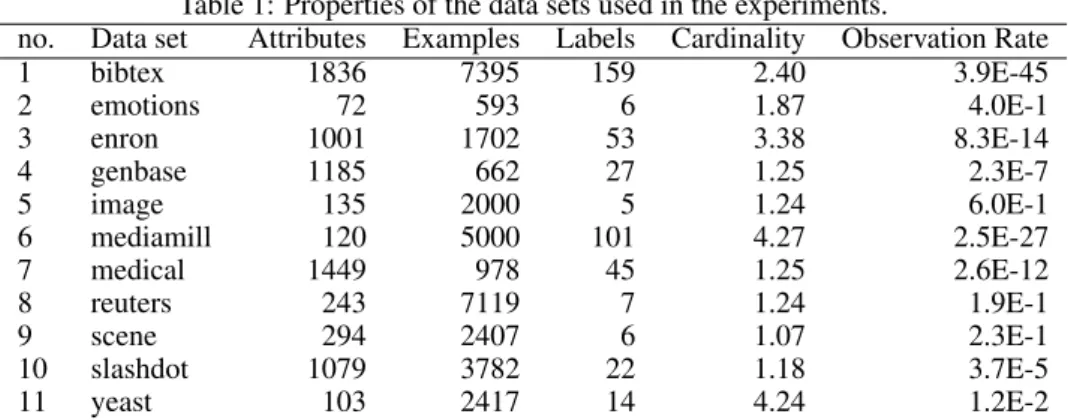
Our second modification is motivated by the observation that the number of label combinations that are commonly observed in MLC data sets is only a tiny fraction of the total number |Y| = 2m of possible subsets; see Table 1,
which reports the value|YD|2−m, whereYD is the set of
unique label combinations contained in the dataD, as the “observation rate” in the last column. Moreover, if a label combinationyhas an occurrence probability of >0, then the probability that it has never be seen in a data set of size
nreduces to(1−)n. Thus, by contraposition, one may
argue that such a label combination is indeed unlikely to exist at all (at least for large enoughn).
Our idea of “subset correction”, therefore, is to restrict a learner to the prediction of label combinations whose exis-tence is testified by the (training) data. More precisely, let
YS denote the set of label subsetsythat have be seen in
the training dataS. Then, given a predictionyˆproduced by a classifierh, this prediction is replaced by the “most similar” subsety∗∈ Y S: y∗∈argmin y0∈Y S LH(yˆ,y0) (7)
Thus,y∗ is eventually returned as a prediction instead of
ˆ
y. If the minimum in (7) is not unique, those label combi-nations with higher frequency in the training data are pre-ferred.
In principle, the Hamming loss could of course be re-placed by other MLC loss functions in (7). Its use here is mainly motivated by the fact, that it is used for a similar purpose, namely decoding, in the framework oferror cor-recting output codes(ECOC). As such, it has been applied in multi-class classification [?] and lately also in MLC [9; 7].
6
Nested Stacking vs. Classifier Chains
In this section, we compare NS and CC, both with and without subset correction, on real MLC benchmark data. As can be seen in Table 1, the data sets differ quite sig-nificantly in terms of the number of attributes, examples, labels, cardinality (number of labels per example) and the observation rate.Logistic regression was used as a base learner for binary prediction in all MLC methods [10]. Unlike [13], we do not apply any threshold selection procedure; instead, we simply usedt= 0.5for deciding the relevance of a label. In fact, our goal is to study the behavior of CC and NS without the influence of other factors that may bias the results.
Since CC’s main goal is to detect conditional label de-pendence, we used example-based metrics for evaluation.
In addition to Hamming and subset 0/1 loss introduced ear-lier, we also applied theF1and Jaccard index defined, re-spectively, as follows (note that these are accuracy mea-sures instead of loss functions):
F1(y,h(x)) = 2Pm i=1[[yi= 1andhi(x) = 1]] Pm i=1([[yi= 1]] + [[hi(x) = 1]]) (8) J accard(y,h(x)) = Pm i=1[[yi= 1andhi(x) = 1]] Pm i=1[[yi= 1orhi(x) = 1]] (9) The value for a test set is defined as the average over all instances. The scores reported in Tables 2 and 3 were esti-mated by means of 10-fold cross-validation, repeated three times. We used a paired t-test for establishing statistical significance on each data set.
Table 4: The effect of subset correction in terms of sta-tistical significance. The corresponsing loss/accuracy val-ues can be found in Tables 2-3. () means that NSSC
(CCSC) is significantly better (worse) than NS (CC) at level
p <0.01(↑and↓at levelp <0.05) in a paired t-test.
NS vs. NSSC
no. m Hamming Subset 0/1 Jaccard F1
1 159 2 6 3 53 4 27 5 5 6 101 7 45 ↑ 8 7 9 6 10 22 11 14 CC vs. CCSC
no. m Hamming Subset 0/1 Jaccard F1
1 159 2 6 ↑ 3 53 4 27 5 5 6 101 7 45 8 7 9 6 ↓ 10 22 11 14
Looking at the comparison between CC and NS (without subset correction) as shown in Table 2), the first thing to mention is the strong performance of NS in terms of Ham-ming loss (8 significant wins and 3 losses). In terms of their properties, the three data sets on which NS looses do indeed seem to be favorable for CC: Since slashdot, med-ical and genbase all have a rather low Hamming loss, the danger of error propagation is limited. Thus, the results are completely in agreement with our expectations.
For Jaccard and F1, the picture is not as clear. In both cases, NS wins 6 times. Again, like for Hamming loss, NS
Table 1: Properties of the data sets used in the experiments.
no. Data set Attributes Examples Labels Cardinality Observation Rate
1 bibtex 1836 7395 159 2.40 3.9E-45 2 emotions 72 593 6 1.87 4.0E-1 3 enron 1001 1702 53 3.38 8.3E-14 4 genbase 1185 662 27 1.25 2.3E-7 5 image 135 2000 5 1.24 6.0E-1 6 mediamill 120 5000 101 4.27 2.5E-27 7 medical 1449 978 45 1.25 2.6E-12 8 reuters 243 7119 7 1.24 1.9E-1 9 scene 294 2407 6 1.07 2.3E-1 10 slashdot 1079 3782 22 1.18 3.7E-5 11 yeast 103 2417 14 4.24 1.2E-2
Table 2: Experimental results of NS and CC on benchmark data sets.() means that NS is significantly better (worse) than CC at levelp <0.01(↑and↓at levelp <0.05) in a paired t-test.
F1 JACCARDINDEX no. m CC NS CC NS 1 159 0.1697±.0071 0.1747±.0077 0.1098±.0060 0.1133±.0064 2 6 0.5883±.0534 0.6028±.0500 ↑ 0.5003±.0521 0.5144±.0514 ↑ 3 53 0.3483±.0191 0.3729±.0214 0.2474±.0163 0.2693±.0178 4 27 0.9863±.0090 0.9854±.0085 ↓ 0.9804±.0115 0.9789±.0109 ↓ 5 5 0.5556±.0284 0.4780±.0299 0.5196±.0271 0.4460±.0278 6 101 0.5326±.0054 0.5619±.0053 0.4280±.0052 0.4459±.0052 7 45 0.6462±.0331 0.6444±.0340 0.5828±.0343 0.5804±.0356 8 7 0.8599±.0128 0.8570±.0116 0.8336±.0138 0.8302±.0129 9 6 0.5969±.0403 0.6031±.0348 0.5745±.0405 0.5766±.0344 10 22 0.3278±.0185 0.3259±.0186 0.2747±.0176 0.2726±.0180 11 14 0.5836±.0182 0.6068±.0172 0.4848±.0198 0.4990±.0183
HAMMINGLOSS SUBSET0/1 LOSS
no. m CC NS CC NS 1 159 0.0724±.0020 0.0672±.0016 0.9837±.0052 0.9833±.0052 2 6 0.2367±.0268 0.2169±.0253 0.7578±.0575 0.7477±.0633 3 53 0.1233±.0051 0.1050±.0051 0.9565±.0135 0.9510±.0133 ↑ 4 27 0.0019±.0011 0.0020±.0010 ↓ 0.0408±.0211 0.0443±.0213 ↓ 5 5 0.2104±.0127 0.1962±.0119 0.5857±.0269 0.6468±.0249 6 101 0.0303±.0004 0.0291±.0004 0.8752±.0049 0.8969±.0048 7 45 0.0248±.0031 0.0249±.0031 0.5890±.0425 0.5934±.0463 8 7 0.0506±.0046 0.0483±.0043 0.2454±.0173 0.2499±.0175 ↓ 9 6 0.1470±.0143 0.1397±.0124 0.4918±.0434 0.5019±.0355 ↓ 10 22 0.0908±.0027 0.0913±.0028 ↓ 0.8652±.0185 0.8678±.0198 11 14 0.2242±.0093 0.2069±.0087 0.8104±.0229 0.8469±.0231
outperforms CC on data sets with many labels (bibtex, en-ron, mediamill) or a relatively high Hamming loss (yeast), whereas CC is better for data sets with only a few labels (image, reuters) or with high accuracy (genbase).
The picture for CC and NS with subset correction (de-noted CCSC and NSSC, respectively) is quite similar
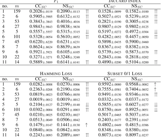
(Ta-ble 3), although the performance differences tend to de-crease in absolute size. On subset 0/1 loss, for which the original CC performs quite strong and typically out-performs NS, the corrected version NSSC even achieves 3
significant wins over CCSC.
To analyze the effect of subset correction in more detail, Table 4 provides a summary of a comparison of Table 2 and Table 3. Interestingly enough, subset correction yields im-provements on almost every experiment, regardless of the performance measure, and most of these improvements are even significant. More specifically, counting the number of significant wins, subset correction appears to be most
ben-eficial for subset 0/1 loss and least benben-eficial for Hamming loss. In fact, for Hamming loss, subset correction looses for data sets with only a few labels (reuters, scene, yeast and image) and a relatively high observation rate. Comparing NS and CC, the former seems to benefit even more from subset correction than the latter, except for Hamming loss, on which NS is already strong in its basic version. In terms of subset 0/1 loss, however, significant improvements can be seen on every single data set. In light of the simplicity of the idea, these effects of subset correction are certainly striking.
7
Conclusions
This paper has thrown a critical look at the classifier chains method for multi-label classification, which has been adopted quite quickly by the MLC community and is now commonly used as a baseline when it comes to com-paring methods for exploiting label dependency.
Notwith-Table 3: Experimental results of NSSC and CCSC on benchmark data sets.() means that NSSC is significantly better
(worse) than CCSCat levelp <0.01(↑and↓at levelp <0.05) in a paired t-test.
F1 JACCARDINDEX no. m CCSC NSSC CCSC NSSC 1 159 0.2026±.0119 0.2090±.0113 0.1528±.0099 0.1582±.0100 2 6 0.5905±.5905 0.6132±.6132 0.5027±.0521 0.5239±.0525 3 53 0.3843±.3843 0.4016±.4016 0.2821±.0190 0.3005±.0238 4 27 0.9843±.9843 0.9838±.9838 0.9807±.0129 0.9802±.0125 5 5 0.5557±.5557 0.5315±.5315 0.5197±.0272 0.4972±.0304 6 101 0.5328±.0054 0.5610±.0052 0.4282±.0052 0.4457±.0050 7 45 0.6220±.6220 0.6231±.6231 0.5898±.0435 0.5900±.0460 8 7 0.8624±.8624 0.8639±.8639 0.8367±.0142 0.8382±.0126 9 6 0.5921±.5921 0.6105±.6105 0.5739±.0423 0.5873±.0370 10 22 0.3271±.3271 0.3248±.3248 0.2843±.0186 0.2818±.0202 11 14 0.5889±.5889 0.6141±.6141 0.4890±.0200 0.5104±.0200
HAMMINGLOSS SUBSET0/1 LOSS
no. m CCSC NSSC CCSC NSSC 1 159 0.0282±.0008 0.0270±.0006 0.9592±.0080 0.9568±.0082 ↑ 2 6 0.2363±.0268 0.2190±.0266 0.7555±.0581 0.7404±.0652 ↑ 3 53 0.0819±.0023 0.0766±.0030 0.9491±.0130 0.9346±.0156 4 27 0.0019±.0012 0.0019±.0012 0.0332±.0176 0.0337±.0172 5 5 0.2104±.0127 0.2199±.0140 0.5855±.0270 0.6027±.0277 6 101 0.0302±.0004 0.0291±.0003 0.8750±.0049 0.8925±.0051 7 45 0.0210±.0025 0.0210±.0027 0.5017±.0465 0.5037±.0514 8 7 0.0513±.0049 0.0506±.0042 0.2403±.0177 0.2391±.0167 9 6 0.1479±.0147 0.1441±.0130 ↑ 0.4802±.0449 0.4815±.0386 10 22 0.0840±.0026 0.0842±.0028 0.8348±.0186 0.8380±.0201 11 14 0.2243±.0093 0.2089±.0097 0.8073±.0230 0.8097±.0237
standing the appeal of the method and the plausibility of its basic idea, we have argued that, at second sight, the chain-ing of classifiers begs an important flaw: A binary classi-fier that has learnt to rely on the values of previous labels in the chain might be misled when these values are replaced by possibly erroneous estimations at prediction time. The classification errors produced because of this attribute noise may subsequently be propagated or even reinforced along the entire chain. Roughly speaking, what looks as a gift at training time may turn out to become a handicap in predic-tion.
Our results have shown that the problem of error prop-agation is highly relevant, and that it may strongly impair the performance of CC. In order to avoid this problem, the method of nested stacking proposed in this paper uses pre-dicted instead of observed label relevances as additional at-tribute values in the training phase. Our experimental stud-ies clearly confirm that, although NS does not consistently outperform CC, it seems to have advantages for those data sets on which error propagation becomes an issue, namely data sets with many labels or low (label-wise) prediction accuracy.
There are several lines of future work. First, it is of course desirable to complement this study by meaningful theoretical results supporting our claims. Second, it would be interesting to investigate to what extent the problem of attribute noise also applies to the probabilistic variant of classifier chains introduced in [3]. Last but not least, given the interesting effects that are produced by the simple idea of subset correction, this approach seems to be worth fur-ther investigation, all the more as it is completely general and not limited to specific MLC methods such as those con-sidered in this paper.
References
[1] Gert Cauwenberghs and Tomaso Poggio. Incremen-tal and decremenIncremen-tal support vector machine learning.
Proc. NIPS, pages 409–415, 2001.
[2] W. Cheng and E. H¨ullermeier. Combining instance-based learning and logistic regression for multilabel classification. Machine Learning, 76(2-3):211–225, 2009.
[3] K. Dembczy´nski, W. Cheng, and E. H¨ullermeier. Bayes optimal multilabel classification via probabilis-tic classifier chains. InICML, pages 279–286, 2010. [4] K. Dembczy´nski, W. Waegeman, W. Cheng, and
E. H¨ullermeier. On label dependence and loss minimization in multi-label classification. Machine Learning, To appear, 2012.
[5] A. Elisseeff and J. Weston. A Kernel Method for Multi-Labelled Classification. InACM Conf. on Re-search and Develop. in Infor. Retrieval, pages 274– 281, 2005.
[6] J. F¨urnkranz, E. H¨ullermeier, E.L. Menc´ıa, and K. Brinker. Multilabel classification via calibrated la-bel ranking. Machine Learning, 73:133–153, 2008. [7] Johannes F¨urnkranz and Sang-Hyeun Park.
Error-correcting output codes as a transformation from multi-class to multi-label prediction. In Proc. Dis-covery Science, pages 254–267. 2012.
[8] S. Godbole and S. Sarawagi. Discriminative methods for multi-labeled classification. InPacific-Asia Conf. on Know. Disc. and Data Mining, pages 22–30, 2004. [9] Tomasz Kajdanowicz and Przemysław Kazienko. Multi-label classification using error correcting
out-put codes. International Journal of Applied Mathe-matics and Computer Science, 22(4):829–840, 2012. [10] C.-J. Lin, R. C. Weng, and S. S. Keerthi. Trust
re-gion Newton method for logistic regression. Jour-nal of Machine Learning Research, 9(Apr):627–650, 2008.
[11] E. Monta˜n´es, J. R. Quevedo, and J. J. del Coz. Ag-gregating independent and dependent models to learn multi-label classifiers. InProc. ECML/PKDD, 2011. [12] J. Read, B. Pfahringer, and G. Holmes. Multi-label
classification using ensembles of pruned sets. InIEEE Int. Conf. on Data Mining, pages 995–1000. IEEE, 2008.
[13] J. Read, B. Pfahringer, G. Holmes, and E. Frank. Classifier chains for multi-label classification. Ma-chine Learning, 85(3):333–359, 2011.
[14] R. E. Schapire and Y. Singer. Boostexter: A boosting-based system for text categorization. In Machine Learning, pages 135–168, 2000.
[15] Robin Senge, Juan Jos del Coz, and Eyke H¨ullermeier. On the problem of error propagation in classifier chains for multi-label classification. In Con-ference of the German Classification Society, 2012. [16] G. Tsoumakas, I. Katakis, and I. Vlahavas. Mining
multi-label data. InData Mining and Knowledge Dis-covery Handbook, pages 667–685. 2010.
[17] G. Tsoumakas and I. Vlahavas. Random k-Labelsets: An Ensemble Method for Multilabel Classifica-tion. InProc. ECML/PKDD, LNCS, pages 406–417. Springer, 2007.
[18] D. H. Wolpert. Stacked generalization. Neural Net-works, 5:214–259, 1992.
[19] M.-L. Zhang and Z.-H. Zhou. Multilabel neural net-works with applications to functional genomics and text categorization. IEEE Trans. on Knowl. and Data Eng., 18:1338–1351, 2006.
[20] X. Zhu and X. Wu. Class noise vs. attribute noise: a quantitative study of their impacts. Artificial Intelli-gence Review, 22(3):177–210, 2004.