Unsupervised Anomaly Detection in Unstructured Log-Data for Root-Cause-Analysis

(1)

BERKAY KICANAOGLU

UNSUPERVISED ANOMALY DETECTION

IN UNSTRUCTURED LOG-DATA FOR ROOT-CAUSE-ANALYSIS

Master's Thesis

Examiner: Prof. Moncef Gabbouj Examiner and topic approved by the Faculty Council of the Faculty of Computing and Electrical Engineering on 4 March 2015

(2)

i

ABSTRACT

BERKAY KICANAOGLU: Unsupervised Anomaly Detection in unstructured log-data for root-cause-analysis

Tampere University of Technology

Master's Thesis, 64 pages, 0 Appendix pages April 2015

Master's Degree Programme in Information Technology Major: Signal Processing

Examiner: Prof. Moncef Gabbouj

Keywords: anomaly detection, density-based clustering, neural networks, support vector data description, pattern recognition, machine learning,data mining

Anomaly detection has attracted the attention of researchers from a variety of back-grounds as it nds numerous applications in the industry. As a subeld, fault detection plays a crucial role in growing telecommunications networks since failures lead to dissatisfaction and hence nancial drawbacks. It aims at identifying unusual events in the system log les. System logs are messages from the elements of the net-work to highlight their status. The main challenge is to cope with the rate the data volume grows. Traditional methods such as expert systems are no longer practical making machine learning approaches more valuable.

In this thesis work, unsupervised anomaly (fault) detection in unstructured system logs is investigated. The eect of various feature extraction methods are investi-gated in terms of the gain they provide. Also, the baseline dimensionality reduction method Principal Component Analysis (PCA) and its eects are given. Addition-aly, autoencoders are studied as an alternative dimensionality reduction technique. Four dierent methods based on statistics and clustering as well as a framework to clean datasets from anomalies are discussed. A high detection (classication) rate with99.69%precision and0.07% false alarm rate are achieved in one of the datasets

while similar results have been achieved with variations in the recall in the other dataset. The studies show that the dimensionality reduction can greatly improve the performance of the classiers used and reduce the computational complexity in anomaly detection.

(3)

ii

PREFACE

This work has been conducted at the Department of Signal Processing of Tampe-re University of Technology in collaboration with TIETO within ICT SHOK D2I project.

I would like to express my gratitudes to my supervisor Prof. Moncef Gabbouj for engaging me in such an exciting subject and for the support throughout the thesis. Furthermore, I believe I owe Honglei Zhang and Stefan Uhlmann big thanks for they contributed in this work with their valuable opinions, comments and guidance. Also, I would like to thank Alexandros Iosidis for bringing a dierent perspective to the thesis and being very supportive.

There are many other to thank for being there when things got out of hand. However, my friends with whom I shared a lot deserves a huge warm thanks for their friendship and support. In addition to those, special thanks go to my team mates and coaches with whom we shared pain, fun and, of course, glorious victories.

Finally, I would like to thank my family for being there no matter what. Their belief and support always make me go one step ahead from where I am.

Berkay Kicanaoglu Tampere, June 2015

(4)

iii

LIST OF FIGURES

2.1 Basic building blocks of a pattern classier . . . 4

2.2 Common evaluation metrics in the context of anomaly detection . . . 9

2.3 Neuron: Elementary unit of Articial Neural Networks . . . 17

2.4 Commonly used activation functions . . . 17

2.5 Example autoencoder conguration . . . 18

3.1 Visualisation of the datasets in 2D space . . . 29

3.2 The-neighborhood . . . 32

3.3 Illustration of core and reachability distances . . . 34

3.4 Two-tier anomaly removal framework . . . 41

4.1 Illustration of log lines . . . 43

4.2 TTY2-500k dataset in 3D space . . . 43

4.3 Eect of dimensionality reduction in naive Bayesian approach . . . . 46

4.4 The performance of Naive Bayesian method w.r.t. the number of principal components . . . 47

4.5 Comparison of dierent features . . . 48

4.7 Histograms of kth neighbor distances . . . 51

4.8 The variation of performance values against the number of principal components used . . . 52

4.9 The eect of dierent feature types in classication performance . . . 52

4.10 ROC curves for dierent window sizes . . . 53

(7)

vi

4.12 The eect of the parameter M inP tsin OPTICS-based approach . . . 55

4.13 The eect of the window size for OPTICS-based approach . . . 56

4.14 Comparison of feature types . . . 57

4.15 The dimensionality reduction scheme using autoencoders . . . 58

4.16 The representation of the TTY dataset by autoencoders . . . 59

4.17 K-means precision histogram . . . 60

4.18 K-means recall histogram . . . 60

(8)

vii

LIST OF TABLES

2.1 Various works used in numerous anomaly detection applications . . . 12 4.1 Fault Types . . . 42 4.2 The parameters that are kept constant . . . 45 4.3 The network parameters used . . . 57 4.4 The number of samples from each class before and after the anomaly

removal . . . 61 4.5 Comparison of classication performances for TTY dataset . . . 62 4.6 Comparison of classication performances for TTY2 dataset . . . 62

(9)

viii

LIST OF ABBREVIATIONS AND SYMBOLS

ANN Articial Neural Network

AUC Area Under Curve

BoL1 Bag-of-lines (Legal Word Selection Rule Set-1) BoL1 Bag-of-lines (Legal Word Selection Rule Set-2)

BoW Bag-of-words

CD Core Distance

DB Density-based

DOS Density Outlier Score

FAR False Alarm Rate

FN False Negative

FP False Positive

KNN K-nearest Neighbors

KL Kullback-Leibler

KSVDD Kernel Support Vector Data Description

LD Local Density

LOF Local Outlier Factor

ML Maximum Likelihood

NB Naive Bayesian

N P-hard Nondeterministic Polynomial Time-hard

OPTICS Ordering Points to Identify the Clustering Structure

OS Outlier Score

PCA Principal Component Analysis

RD Reachability Distance

ROC Receiver Operating Characteristic SVDD Support Vector Data Description

SVM Support Vector Machines

TN True Positive

TP True Negative

w.r.t. with respect to

a center vector of the data description, page 36

b bias value, page 17

β parameter controlling the sparsity constraint, page 18

c class label, page 25

C set of all possible classes, page 25

(10)

ix g number of clusters, page 6

h mapping function, page 5

hW,b(.) hypothesis function learnt by the autoencoder given W and b, page 17

D data set, page 5

J(.) squared error cost function, page 18

Jsparse(.) squared error cost function with sparsity constraint, page 18 p(.) probability, page 6

p(.;,) joint probability, page 6

Pr(.|.) conditional probability, page 25

πi mixing proportion associated with an indexed component, page 6 θi parameter vector associated with an indexed component, page 6 θc_i conditional probability Pr(xi |c), page 25

parameter to determine the radius of neighborhood, page 32 λ weight decay parameter, page 18

k number of nearest neighbors, page 30

M inP ts minimum number of points to form a cluster, page 32 N(.) -neighborhood of a sample, page 32

ρ sparsity parameter, page 18 αi lagrange multiplier, page 36 γi lagrange multiplier, page 36

ˆ

ρj average activation in an indexed neuron in the hidden layer, page 18

ξi slack variable to introduce exibility in data description boundary, page 36

L log-likelihood, page 5

L error function, page 36

P linear transformation matrix, page 13

Ri the radius of the sphere w.r.t. an indexed sample, page 30 R the radius of the data description, page 36

µi expected value of an indexed feature, page 14 σ2_i,j covariance of two indexed features, page 14

SX covariance matrix associated with the data matrix, page 14

sl number of neurons in lth layer, page 18

σ smoothing parameter for the RBF kernel, page 39

x multi-dimensional vector, page 4

xi ith (scalar) feature of a multi-dimensional vector x, page 4 x(i) multi-dimensional vector associated with an index, page 17 xi multi-dimensional vector associated with an index, page 5

(11)

x

x∗ novel multi-dimensional vector, page 25

X input space, page 5

X matrix containing data (row-major), page 13

yi label associated with an index, page 5

Y category space, page 5

(12)

1

1. INTRODUCTION

The advances in electronics and multimedia technologies in past few decades coined a new term referred to as 'Big Data'. As use of smart devices and social media becomes a cornerstone in our lives, the amount of data generated and stored every day rises up to unprecedented gures. Big Data refers to this type of very high-volume data sets which cause the traditional software tools to fail in management and interpretation of the content. As a consequence of the emerging 'Big Data' notion, the role of eective multimedia information retrieval and recognition of patterns becomes more vital. Anomaly detection is a eld of interest in pattern recognition dealing with all possible forms of data such as text, image and audio.

Anomaly detection aims to identify certain events which do not conform with the general patterns in the data sets. It is a popular topic in the academia since it nds extensive use in many engineering disciplines and industry. A small subset of applications can be listed as fraud detection, intrusion detection and fault detection. There exist numerous methods proposed in pattern recognition and machine learning elds addressing these problems. The methods that fall into unsupervised learning category should be investigated and tailored for textual data. An up-to-date survey on the various proposals in literature can be found in [43].

1.1 Anomaly Detection

Anomaly (outlier) detection is a signicant problem which has been studied in the domains of pattern recognition and machine learning. Various anomaly detection techniques have been proposed for certain tasks such as fraud detection [23], cyber-intrusion detection [29], fault detection [35, 57], industrial damage detection [32] and image processing [7]. Since the problems vary in the nature of data as well as the domain of application, dierent methods from machine learning and pattern recognition have been studied along with dierent signal processing approaches. Analysis of textual data can be associated with many interesting industrial and daily life problems. For instance, anomaly detection can be used to bring users the novel news headlines or documents in a search engine or it can be exploited to identify

(13)

1.2. Objectives of the Thesis 2 possibly spam emails by a service provider. More specically, anomaly detection can also be used for fault detection in large-scale systems such as telecommunication networks. In this work, unstructured system logs have been delved into, in order to reveal anomalous behavior exhibited by the elements of a telecommunications network.

System logs are in fact time-series signals although they may not necessarily be sampled uniformly in terms of time. However, they contain large amount of infor-mation to be extracted, especially when the data size grows to an extent which is burdensome to handle manually. Hence, it is obvious that research for ecient methods is necessary.

1.2 Objectives of the Thesis

The objectives of this thesis consist of understanding the nature of the data (un-structured system logs), searching for useful feature representations and understan-ding the existing methods and concepts in unsupervised domain in order to apply on the given datasets. Additionally, the objectives include studying dimensionality reduction methods for low-dimensional manifolds determination for enhancing the performance of anomaly detection methods in general and comparing the perfor-mance of various methods.

1.3 Results of the Thesis

The main results for this thesis are that:

• conventional feature extraction method for textual data, bag-of-words, can be replaced by an analogous method bag-of-lines to improve the results for the given problem.

• scoring-based techniques can lead to very good results by allowing more exi-bility for the analyst to focus on the most relevant anomalies in this problem. • dimensionality reduction is crucial for both time eciency and performance.

1.4 Structure of the Thesis

The organization of the thesis is as follows. Chapter 2 presents a literature over-view on pattern recognition, anomaly detection, dimensionality reduction methods

(14)

1.4. Structure of the Thesis 3 and evaluation techniques. Chapter 3 gives more detailed description of the used methods including other building blocks such as preprocessing and feature extrac-tion. Chapter 4 provides the evaluation of methods in terms of parameters and performance. Finally, the thesis is concluded in Chapter 5 by discussions and future research plans.

(15)

4

2. THEORETICAL BACKGROUND

This chapter provides the basic knowledge for pattern recognition and machine lear-ning concepts that will be used throughout the thesis.

2.1 Pattern Recognition

The term Pattern Recognition refers to the analysis and interpretation of data th-rough discrimination and classication encapsulating all the stages required such as problem formulation and data collection [55](see Fig. 2.1). In simplest words, it aims at nding regularities and patterns in data. Most often, it is used interchan-geably with the term Machine Learning although they dier in certain aspects. However, there exist a sheer amount of overlap in what they cover, making it hard to distinguish the boundaries. They both origin from the articial intelligence with pattern recognition mainly having a greater tendency to formalize and explain the ndings (patterns). In general, a pattern refers tod-dimensional feature vector

x = [x1, . . . , xd]T which corresponds to the measurements/observations for an ob-ject/sample. Hence, the set of measurements (observations) depend on the problem and the investigator. However, it is clear that the choice of features to use aect the performance of any pattern recognition system and must be conducted with care. The handcrafted feature engineering has been lately taken over by automatic feature learners in certain application areas such as object recognition [31, 37].

2.1.1 Learning Paradigms

In pattern recognition, approaches can be mainly categorized into two based on the availability of labels. These categories are named as supervised learning and

Data Collection

(e.g. camera, sensor, microphone) Feature Selection/ Extraction Measurements Classifier Decision Pattern x

(16)

2.1. Pattern Recognition 5 unsupervised learning. The labels are the correct class tag associated with each patternx in the dataset.

Supervised learning algorithms are provided with a set of labeled data instances,D, D =(x1, y1),(x2, y2), . . . ,(xN, yN)

where (xi, yi) is the ith pattern-label pair and N is the total number of patterns (samples). In general, it is referred to as training set. This mapping actually denes a function h : X → Y. The task for the learner is to determine an approximating function g : X → Y which can produce a mapping from input space to category space as accurate as possible w.r.t.h. The algorithms usually model the data sets

ba-sed on the class characterization provided by labels and uses this model information to classify novel patterns by testing them against it. Supervised learning has found various applications via various algorithms such as k-nearest neighbors (KNN), sup-port vector machines (SVM), decision trees and articial neural networks (ANN). Although these algorithms have been proven to be very powerful tools for certain applications, they have particular disadvantages. First, collecting labels may be dif-cult. Especially, when the data volume is exceptionally large as in the 'Big Data', this process becomes extremely expensive. The second is that real world problems do not always contain discriminative labels. On the contrary, many uncertainties and ambiguities exist in them. These disadvantages should be taken into account as well as the advantages when designing a learning machine.

Unlike supervised learning, unsupervised learning aims at nding the underlying structure, i.e. the relationships between points in the dataset in the absence of labels. Hence, these type of algorithms do not have any guidance to measure the quality of their solutions (during modeling the relationships). In comparison with supervised learning schemes, unsupervised learning can be useful when labeling is not possible or dicult. These methods can be used as a preprocessing step for supervised algorithms as they can provide a priori information or prototypes to the learner. However, they may suer to learn in complex cases since there is no supervision. Therefore, once again, the choice of the right approach is data-specic and it must take the nature of the problem under consideration. There exist many methods that fall into this category and clustering is one of the most commonly used techniques. The examples of common clustering methods can be listed as k-means, mean-shift, expectation-maximization etc.

The goal of any clustering algorithm is to discover sets of objects such that the ob-jects in the same set exhibit similarities whereas obob-jects from dierent sets (clusters,

(17)

2.1. Pattern Recognition 6 groups) show dissimilarities. In other words, the goal of clustering is to maximize intra-class similarities while keeping inter-class similarities as low as possible. There is a vast amount of literature on clustering [56]. Most of the early research was con-ducted in the elds of biology and zoology, although clustering methods have been utilized in many elds of science including signal processing and psychology. The clustering approaches can be categorized w.r.t. their characteristics as follows: Hierarchical methods: These clustering procedures are generally used for data sum-marization based on a given dissimilarity matrix. The hierarchy is most often repre-sented by a dendrogram which is a tree diagram. Breaking the dendrogram at a particular level generates a partition of the data set into disjoint groups. This ap-proach is especially useful if one searches for an interactive analysis tool which allows to see the relationships in a datasets at various degrees of linkage. It has been used in many applications such as microarray gene data analysis [24].

Mixture Models: Each dierent cluster in the dataset is assumed to be generated from a distinct probability distribution. The distributions may be of the same di-stribution family (e.g. Gaussian) with dierent parameter set θ or they may be of dierent distributions families. The dataset is then assumed to be described by a nite mixture distribution of the form

p(x) =

g

X

i=1

πip(x;θi)

whereπi are the mixing proportions (

Pg

i=1πi = 1),g is the number of clusters and

p(x;θi) is d-dimensional probability function with a parameter vector θi [55]. The main task is to estimate πi, θi and g. Once they are estimated the clustering is achieved.

Sum-of-squares methods: These are often called as partitioning or centroid-based clustering methods. Their main task is to partition the space into g so that each subspace contains objects from one particular cluster. The methods vary depending on the choice of clustering criterion optimized. In practice, most of the methods nd a local optima since the optimization problem is itselfN P-hard. The popular examples arek-means and fuzzy k-means [39].

Spectral clustering: These methods exploit the eigenvectors of a graph Laplacian to map the data into another space where the underlying structure is easier to capture [38].

(18)

2.1. Pattern Recognition 7

2.1.2 Structure of a Pattern Recognition System

An unsupervised pattern classication system consists of the following functional blocks:

Preprocessing: This block deals with the raw data retrieved from the source. Ba-sically, preprocessing might incorporate numerous signal processing techniques such as smoothing, trimming and ltering depending on the data type (e.g. text, audio, image etc.). It is a crucial step since the raw data may contain many inconsistencies and errors. Additionally, for most of the algorithms, the raw data is not suitable as input and hence it should be formatted into interpretable form by preprocessing. Feature Extraction/Selection: Features are the relevant observations/measurements obtained from the phenomena which are under investigation. Extraction methods vary according to the problem (e.g. object-detection, shape recognition, document classication etc.). It is highly problem-oriented and usually requires sheer amount of eorts to design best-matching features for the given task. Feature selection re-fers to determining the most relevant subset of features which brings about the best representation, for instance, in terms of discrimination. For clustering and classica-tion problems, one desires to have clusters/classes with the highest intra-class and the lowest inter-class similarity to be able to obtain better performance.

Training: In supervised learning, training is commonly used to refer to the initial phase where the training data set which contains the labels is utilized to build class models. These models are then used to classify novel inputs by testing them against the model or models (e.g. used in one-against-all classiers).

Classication: This block realizes the purpose of the system such as clustering, regression or classication depending on the problem. A system can either be de-signed to assign categories for each sample or to gather together points that behave similarly as in clustering.

A classier in general can produce two types of output, namely, labels and scores. The former is used generally to strictly classify the given novel samples into nite number of categories whereas the former can assign probabilities or scores which can show the likelihood of a given sample to belong to a certain category.

2.1.3 Evaluation Methods and Metrics

The evaluation of the performance of pattern recognition systems is as important as the system itself. It is essential to understand the capabilities of all the building

(19)

2.1. Pattern Recognition 8 blocks including preprocessing and feature extraction. In order to ensure that the performance of the classier is stable, one should take into account approach-specic (supervised, unsupervised) and problem-specic properties.

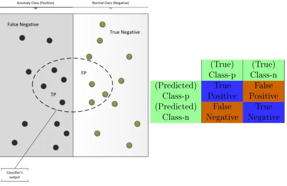
In the eld of machine learning, there exist certain standard evaluation metrics which are commonly used to describe dierent aspects of the systems. The most common forms are accuracy, precision and recall. However, it is hard to select according to which of all the existing measures one should rely on to determine the performance or make a comparison of classication methods. Fig. 2.2 illustrates the major measures in the context of anomaly detection.

• Accuracy describes the ratio of correct classication. It measures how many of samples are assigned to the correct classes and how many are assigned incor-rectly. It is the most common form of performance metrics especially in machi-ne learning. Although it tells about each class, it may fail in class-imbalanced situations as in anomaly detection. Formally, it is dened as follows.

Accuracy= T P +T N

T P +F P +T N +F N

where TP, TN, FP, FN stand for true positive, true negative, false positive and false negative, respectively.

• Precision indicates the rate with which the classier returns the true positives. It is useful, however there is usually a signicant trade-o between precision and recall. Therefore, it is generally not so descriptive of the performance alone. In Fig. 2.2, high precision corresponds to small number of samples from the normal class inside the sphere.

P recision= T P

T P +F P

• Recall measures what percent of the relevant class can be retrieved by the classier. Often it is considered together with precision since there exists a visible trade-o.

Recall = T P

T P +F N

• False Alarm Rate measures how many of the irrelevant class samples are la-beled as relevant. In anomaly detection, false alarm rate refers to the ratio between the number of incorrectly detected normals and total number of nor-mals.

False Alarm Rate= F P

(20)

2.1. Pattern Recognition 9

TP

FP False Negative

True Negative

Anomaly Class (Positive) Normal Class (Negative)

Classifier’s output

(True)

Class-p Class-n(True) (Predicted)

Class-p PositiveTrue PositiveFalse (Predicted)

Class-n NegativeFalse NegativeTrue

Figure 2.2 Common evaluation metrics in the context of anomaly detection.

• Geometric Mean is used to represent two dierent metrics simultaneously (e.g. accuracy and recall). In the scope of this thesis work, it is dened as follows.

Gmean= r T P T P +F N × T N T N+F P

Although these evaluation metrics can provide reasonable amount of information, one can opt for other methods which can be composite of two or more metrics such as Receiver Operating Characteristic (ROC) curves. ROCs can especially be useful in binary classication case when the classier output is score-type. The graph is generated based on the threshold swept through various values. They can be useful when there exists a set of models, methods or parameters involved and a comparison is required. It proves to be more robust against class-imbalancies. Furthermore, the area under the curve (AUC) can also be a good indicator of the performance. However, it may suer since these curves are not unique and multiple methods or parameters can result in the same AUC. This may make drawing a conclusion from them harder.

In supervised learning, there is a problem referred to as overtting which results in low test accuracy (or high test error vice versa) while the training error is low. The problem is due to system's over-learning (memorizing) the training data such that making generalizations on the unseen data becomes harder and less accurate. In order to be able to measure system's performance in generalization,k-fold

(21)

cross-2.2. Anomaly Detection 10 validation is used. It simply divides the dataset into k subsets with equal size and uses only one subset at a time for testing while the remaining k−1 sets are used

for training. The results are calculated by averaging over all folds. In addition to ghting with overtting, it can also give better conclusions for stochastic methods by considering the variations due to the random operations within. Hence, it is a common practice to cross-validate in machine learning.

2.2 Anomaly Detection

Anomaly detection refers to nding non-conforming patterns to normal behavior which is dened by the problem under consideration. These patterns which do not resemble the target (normal) behavior have found many terms such as anomalies, outliers, exceptions, surprises, pecularities and contaminants in many disciplines. However, the terms anomaly and outlier are most commonly used interchangeably. Anomaly detection has been a popular research topic and has great importance in many application domains such as fraud detection, intrusion detection, health care, fault detection and etc.

One of the main reasons why anomaly detection lies at the heart of many critical tasks is that these patterns can be translated into an actionable information im-mediately [13]. In a computer network, an anomaly may correspond to a hacked computer which leaks condential information to unauthorized computers [34]. In credit card transaction data, anomalies can indicate possible fraud attempts [2]. Fi-nally, in the context of this work, anomalies may correspond network elements such as an antenna which is malfunctioning or has broken down.

Anomaly detection faces many diculties arising from the variations in denition of anomaly in the application domain or its abstract notion. In very simple words, it deals with nding the patterns that do not conform to the expected normal behavior. Following this notion, a very straight-forward method would attempt to determine the boundary around the normal points excluding the outliers. However, things might get complicated due to the following reasons listed in [13].

• Dening a very discriminative region for the normal behavior might be imprac-tical since the boundary between normal and anomaly classes can be vague. A normal point very close to this boundary can be anomaly or vice versa. • In case of malicious anomalies such as software viruses, dening the boundary

becomes challenging since these malicious activities can disguise themselves as normal.

(22)

2.2. Anomaly Detection 11 • The normal behavior might not be static, i.e. it can evolve in time, making

the normal representation useless over time.

• The denition of anomaly varies from domain to domain. For instance, small variations in medical data can imply anomaly while similar uctuations fall into normal behavior in weather forecasting. Hence, it becomes less straight-forward to adapt an algorithm from another domain into the problem domain. • The lack of labeled data for training is a major problem.

As a consequence of the given problems, anomaly detection becomes hard to tackle. Almost every problem brings their own formulation leading to hardships for methods to produce a generalized solution.

On top of the conceptual diculties in denition of what is normal or not, anomalies show diversity in type making everything more complicated. There are three major types of anomalies to be considered when designing an anomaly detection system since the type (characteristic) of anomalies being targeted determines the approach to be developed.

• Point anomalies corresponds to data samples which qualify as anomaly with respect to the rest of the data set. It is the simplest type on which the most of the research has been focused. To illustrate, one can imagine a transaction of $1000 as anomaly for a bank account which typically deals with relatively

small amounts such as $50-100.

• Contextual (conditional) anomaly refers to an anomalous behavior which is considered as an anomaly only in certain contexts and not in others. For example, a temperature recording, say 45◦_{C can be considered as an} ano-maly during winter whereas it might be ordinary (normal) for a day during summer.

• Collective anomalies refers to collections of data samples which are anomalous altogether. For instance, in an electrocardiogram output, individual samples with low signal amplitudes may not represent anomalous behavior whereas a collection of similar samples in a consecutive manner can correspond to a collective anomaly.

2.2.1 Anomaly Detection in Unstructured System Log Files

The anomaly detection task in unstructured log les is to identify network compo-nents which signal unexpected signs such as malfunctioning and deactivation. The

(23)

2.2. Anomaly Detection 12 root-cause of a problem can be assumed to stem from the logical or physical neigh-borhood. Hence, in a real setting, the logs reported by physically or logically con-nected elements should reect the situation ongoing in the subgraph (subnetwork). If one can localize the problem by the help of the symptoms broadcast via the logs, then one can get closer to understanding the root-cause.

Unstructured system logs constitutes a time-series signal in which individual lines (logs) do not imply anomalous behavior. The anomalies show themselves in a collec-tive manner but not necessarily sequentially. Unlike host-based intrusion detection systems it is not possible to track sequences of logs to lead to a conclusion, however comparison of the sequences via histograms can bring about solutions.

The key challange in this domain is that the data is in streaming fashion leading to extremely large volumes as in intrusion detection. Therefore it requires ecient on-line analysis methods. Another problem encountered is the false alarm rate due to the large volume of the data. Even very small false alarm rates can cause trouble for the analyst. Hence, the system must be developed such that false alarms are reduced to acceptable levels.

2.2.2 Methods Used in Anomaly Detection

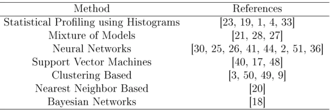
As explained earlier, the problem denition diers in dierent applications, so do the techniques used. In the literature, many have developed various methods according to the data type and the task. Table 2.1 lists some of the approaches and their applications in a compact way. Some of these techniques require labels (supervised) while some do not such as clustering-based techniques.

Method References

Statistical Proling using Histograms [23, 19, 1, 4, 33]

Mixture of Models [21, 28, 27]

Neural Networks [30, 25, 26, 41, 44, 2, 51, 36] Support Vector Machines [40, 17, 48]

Clustering Based [3, 50, 49, 9]

Nearest Neighbor Based [20]

Bayesian Networks [18]

(24)

2.3. Transformations 13

2.3 Transformations

Sometimes, the available features may not serve well in terms of the resulting perfor-mances. This may happen when the true dimensionality of the data is lower than the dimensionality of the data representations, i.e. when the samples lie on a manifold. Dimensionality reduction may become extremely helpful in certain cases in which the algorithms can not model the normal data class against the outlier (anomaly) class well enough. These methods provide more compact and robust representations based on the original feature vectors. In this section, Principal Component Analysis (PCA), which is a baseline method for dimensionality reduction, and autoencoders, a special subcategory of neural networks, will be covered.

2.3.1 Principal Component Analysis (PCA)

Principal component analysis is one of the most widely used unsupervised dimen-sionality reduction methods. Although PCA, in the very basic terms, attempts to describe the data based on a new linear combination of its basis vectors, the orde-ring of the new basis vectors according to how principal they are makes it a viable method to reduce the dimensionality.

To formally express the idea, dene X, Y to be m×n matrices and P to be an

m×m matrix. One can see matrix X as the original feature matrix while Y is the

reexpression of X related by the linear transformation P. Letting columns of X

represent samples and rows represent features (attributes), one can express this transformation as

PX=Y (2.1)

Let pi be the ith row of P and let xi and yi be the ith column of X and Y,

respectively. PX=     p1 ... pm     h x1· · ·xn i Y =     p1·x1 · · · p1·xn ... ... ... pm·x1 · · · pm·xn    

Hence each element of yi is the dot product of corresponding row of P and xi. If

the Eq. 2.1 is considered as change of basis, thenyi is the projection ofxi onto the

(25)

2.3. Transformations 14 In order to determine the best re-expression forX, generally the covariance matrix

is used. Covariance matrix is adequately descriptive to provide all the required in-formation about the features and their interrelations. For better representation of the data, the noise and redundancies should be minimized or removed if possible. Redundancy here may imply that there exist features that are highly correlated and hence some of them can be expressed in terms of the others.

One way to decorrelate the data is to diagonalize the covariance matrix by eigen-vector decomposition. However, to be able to use it properly, one should manipulate the dataset by extracting the mean from each feature so that it is in mean deviation form, i.e. zero mean. For the sake of clarity in the rest of the section, letxi denote

all the observations related to the ith feature (e.g. ith row of X). Then,

V ar[xi] =E[(xi−µi)2] (2.2) whereµi is the expectation ofxi and equal to zero. Therefore,

V ar[xi] =σ2i =E[xixi] (2.3)

In the same spirit, one can show that covariance is equal to the following.

Cov[xi, xj] =σi,j2 =E[xixj] (2.4)

There are two important properties of covariance which will be useful. 1. σ_i,j2 = 0, when featuresi and j are completely uncorrelated. 2. σ_i,j2 =σ_i2, if i=j.

Since xi is dened as row vector, one can calculate covariance with dot product

where expectation is substituted by normalization. Cov[xi, xj] =σ2i,j =

1

n−1xix

T

j (2.5)

Using Eq. 2.5, one can show that covariance matrix of X is

SX =

1

n−1XX

(26)

2.3. Transformations 15 such that SX =          σ2 1,1 · · · σ12,n σ2 2,1 σ22,2 · · · σ22,n ... ... ... ... ... ... ... · · · σ2 n−1,n−1 σn−2 1,n σ2 n,1 · · · σ2n,n         

As σ_i,j2 = σ_j,i2 by denition of covariance, SX is symmetric. The diagonal entries

of SX are the variances while o-diagonals are the covariances. After this point,

solution of PCA requires the eigenvector decomposition as mentioned earlier. The task is to determineP so that SY is diagonalized given Y =PX.

SY = 1 n−1YY T _(2.7) = 1 n−1(PX)(PX) T _(2.8) = 1 n−1(PXX T PT) (2.9) = 1 n−1P(XX T₎_PT _(2.10) = 1 n−1PAP T _(2.11)

whereA=XXT. With the help of the following theorems from linear algebra, one

can proceed to the solution.

Theorem 1. A matrix is symmetric if and only if it is orthogonally diagonalizable. Theorem 2. A symmetric matrix is diagonalized by a matrix of its orthonormal eigenvectors.

Theorem 3. The inverse of an orthogonal matrix is its transpose. By Thm.2, symmetric matrixA can be diagonalized as

A=EDET (2.12)

(27)

PT and substituting 2.12 into 2.11, SY = 1 n−1PAP T _(2.13) = 1 n−1P(P T_DP₎_PT _(2.14) = 1 n−1(PP T₎_D₍_PPT₎ _(2.15) = 1 n−1(PP −1₎_D₍_PP−1₎ _(2.16) = 1 n−1D (2.17)

P−1 ₌_PT _{in 2.16 is the result of Thm.3. From 2.17 it is clear that PCA diagonalizes} SY given P's rows are eigenvectors of XXT. Since the eigenvalues of D are sorted

w.r.t. their magnitudes, one can use this information to reduce dimensionality. The eigenvectors corresponding to smaller eigenvalues can be omitted without much loss (loss will be proportional to the variance they account for). This will lead toY with

˜

m dimensions such thatm < m˜ .

In this thesis work, PCA is generally applied before the decision-making algorithms in order to obtain more robust results. Using the principal components that cor-respond to the largest variances brings about more insight about the data since dynamics of the phenomenon reveals itself in those directions.

2.3.2 Autoencoders

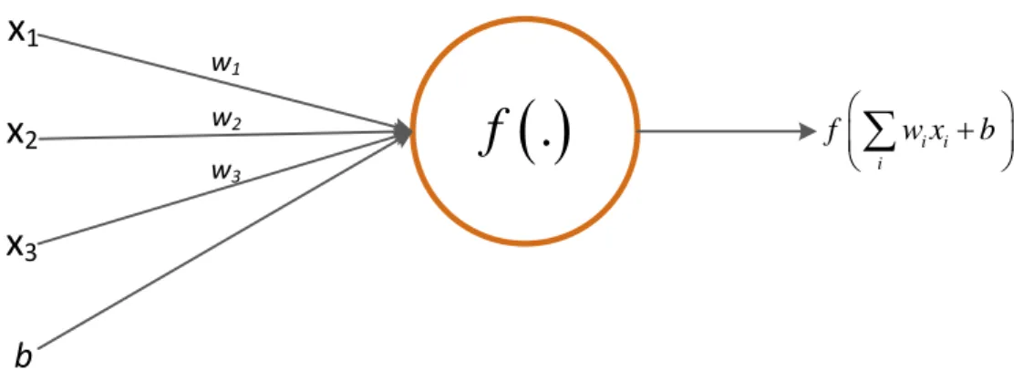
Autoencoders are a subcategory of (feed-forward) articial neural networks (ANN) which possesses auto-association property. It is an unsupervised learning algorithm trained by using backpropagation method [45]. Autoencoders usually have a hidden layer which has less number of neurons compared to visible layers. The main goal of this particular type of networks is to learn how to reconstruct the data from a lower dimensional space representation. Before explaining in further detail, it is useful to dene fundamental building blocks of an ANN.

Neuron

A neuron is the elementary computing unit in neural networks and hence in au-toencoders. It is inspired from the biological structures in the brain which are res-ponsible for learning. The computational counterpart of the biological neurons con-sists of synapse-like components and a body. The synapses have synaptic weights or weights which determine the output of a neuron. The neuron computes the product WT_x _where _x _{∈ <}n_{. However, the output of a neuron is usually determined by a}

(28)

x

1

x

2

x

3

b

w1 w2 w3 i i i f _ w x b_ 





 

.

f

Figure 2.3 Neuron: Elementary unit of Articial Neural Networks (ANN)

f(z) =          1 1 +e−z · · · Sigmoid ez −e−z ez+e−z · · · Tanh

Figure 2.4 Commonly used activation functions

nonlinear activation function f(.) such as sigmoid or tangent-hyperbolic (tanh) as

depicted in Fig. 2.3 and Fig. 2.4. Autoencoder

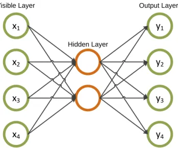
Autoencoders are unsupervised in the sense that labels are not required because the target is the input itself. Due to the shape of conguration as in Fig. 2.5, autoenco-der's task becomes to learn a good representation in a lower dimension imposed by the number of neurons in the hidden layer (bottleneck) so that the reconstruction error at the output is small. Therefore, if the training is successful the autoencoder discovers a new set of features in the bottleneck. In other words, autoencoder tries to learn the identity function which seems trivial unless there are constraints on the size of hidden layer (e.g., <visible layer size).

As a member of feed-forward neural network family, autoencoder has two modes of operation, namely, forward and back propagation. In the former, the input is fed from the input layer and the activations of each neuron are calculated layer-by-layer. The error is calculated at the output and backpropagated. During backpropagation the weights are modied by amounts they account for in the error. In this thesis work, a special type of error function which sets constraints on the activation levels in the hidden layer is used (sparsity condition). In order to explain the dierence between the squared error objective function and the one with the sparsity constraint, denote the dataset as D = n(x(1), y(1)), . . . ,(x(n), y(n))o where (x(i), y(i)) is the ith sample

(29)

x1

x2

x3

x4

y1

y2

y3

y4

Visible Layer Hidden Layer Output Layer

Figure 2.5 Example autoencoder conguration

and its target. Also, denote the hypothesis function the autoencoder learns given the weightsW and biases b as hW,b(x). Then, the squared error cost function becomes

[42]: J(W, b) = 1 n n X i=1 J(W, b;x(i), y(i)) + λ 2 l−1 X l=1 sl X i=1 sl+1 X j=1 (W_ji(l))2 (2.18) J(W, b) = 1 n n X i=1 ||hW,b(x(i))−y(i)||2 + λ 2 l−1 X l=1 sl X i=1 sl+1 X j=1 (W_ji(l))2 (2.19)

where the second term is the weight regularization which makes the network favor smaller weights. The weight decay helps prevent from overtting. The variablesl is the size of lth layer. The parameter λ controls the trade-o between the squared error and the weight decay.

In order to impose the sparsity condition, one should denote the activation of the jth neuron due to input pattern x(i) _{in the hidden layer} _h _with _a(h)

j (x(i)). Then, it is desired to limit the average activation by the sparsity parameter, ρ. The average activation for thejth neuron in the hidden layer in Fig. 2.5 can be calculated as:

ˆ ρj = 1 n n X i=1 a(2)_j (x(i)) (2.20)

(30)

2.3. Transformations 19 divergence, KL(ρ||ρˆj) which is given by:

KL(ρ||ρˆj) =ρlog ρ ˆ ρj + (1−ρ) log 1−ρ 1−ρˆj (2.21) Finally, the cost (objective) function to be minimized becomes:

Jsparse(W, b) = J(W, b) +β s2

X

j=1

KL(ρ||ρˆj) (2.22) whereβ controls the inuence of the sparsity constraint.

The autoencoder using this type of Jsparse(W, b) are referred to as sparse autoenco-ders.

Training of Autoencoders

As in the same fashion with the feed-forward type ANNs, sparse autoencoders can be trained with backpropagation [45]. In the beginning of the training network weights are initialized to small random values. However, the initialization determines the results as gradient-descent or its variants used in backpropagation can get stuck in undesired local minima depending on the initial values. Therefore, pre-training is highly recommended. The pretraining strageties usually involve unsupervised lear-ning approaches. In this way, the network weights are adapted to the properties of the training data. Supervised ne-tuning on top of such an unsupervised learning approach can be used to increase discrimination.

Also, in order to increase the training speed, the inputs should be normalized. This fact results from the partial derivatives which drive the optimization task. When the inputs are large then the derivative of the non-linear function (e.g, sigmoid) becomes too small and it takes more time to converge to the minima.

(31)

20

3. METHODOLOGY

In this chapter, the algorithms which have been used during the experiments and the details of their implementation are given in an elaborate manner. Throughout this chapter, the following steps will be covered respectively: data pre-processing, feature extraction, transformations and classication.

3.1 Data Preprocessing

Most of the pattern recognition/machine learning algorithms usually employ vectors of numerical values, symbols and indicator variables in order to produce a solution for the problem. Therefore, whenever the raw data are not suitable to be immediately fed into the classier/clustering algorithm, the preprocessing need arises.

In problems related to textual data, the general approach is to form dictionary for the most common or relevant words. Hence the preprocessing mainly deals with shaping of the log data to generate a good dictionary. In order for the feature extraction to output powerful representations, the rows (lines) of the system log le should be processed so that certain classes of words or other elements (e.g. ID numbers of network components) are discarded. The point is to extract words that bear useful information.

Based on dierent word selection rules, one can obtain various representations for the data. The purpose of dierent preprocessing methods is to determine the most robust representation leading to a better performance in the decision stages. In the following subsections legal word selection rules utilized are described in algorithmic fashion.

3.1.1 Legal Word Selection Rule Set-1

This procedure ignores any word containing a character which is not an element of the English alphabet. This process is described in Algorithm 1. The features

(32)

3.1. Data Preprocessing 21 generated using this selection rule will be referred to as BoL in the following chapters. Data: Log le

Result: Set of legal words initialization;

legalW ords←− ∅;

while not at the end of le do read current line;

S ←− ∅;

if not empty then

discard the time stamp;

discard all the words containing a character which is not in the English alphabet ;

S ←− eligible words; while S 6=∅ do

if word∈legalW ordsthen do nothing;

else

legalW ords←−word; end S ←−S−word; end else go to next line; end end

Algorithm 1: Word Selection Rule Set-1

3.1.2 Legal Word Selection Rule Set-2

Unlike Legal Word Selection Rule Set-1, this set of rules eliminates only very specic type of words that occurs frequently. These words usually indicate the IDs of network elements which do not necessarily help but increase the size of dictionary.The steps followed for this process is described in Algorithm 2. The features generated using

(33)

3.2. Feature Extraction 22 this selection rule will be referred to as BoL2 in the following chapters.

Data: Log le

Result: Set of legal words initialization;

legalW ords←− ∅;

while not at the end of le do read current line;

S ←− ∅;

if not empty then

discard the time stamp;

discard the words containing '#EID' and/or 'eNodeB'; S ←− eligible words;

while S 6=∅ do

if word∈legalW ordsthen do nothing;

else

legalW ords←−word; end S ←−S−word; end else go to next line; end end

Algorithm 2: Word Selection Rule Set-2

3.2 Feature Extraction

In this section, the details of the feature types and the way they are generated from the data are described.

3.2.1 Windowing

In time-series data analysis, one of the common practices is to partition the data into smaller chunks which are usually called windows. Since the system logs are generated with respect to time, it will be considered as a multi-dimensional time-series signal. Therefore, after the preprocessing step a windowing operation is applied on the logs. At this point, it is reasonable to present two dierent types of windows as follows:

(34)

3.2. Feature Extraction 23 1. Time windows: These windows span certain time frame and are likely to

include distinct number of lines in each window.

2. Fixed-length windows: These windows do not take time frame into account, however contain equal number of lines in every window.

Windowing is done such that the consecutive windows overlap by a rate which is referred to as overlap ratio in general. However, since the experiments did not yield any improvement based on the overlap ratio, we will use an overlap ratio of 33% in

the rest of the thesis.

Throughout the work, features are extracted using the second type (i.e. xed-length) windows. This is due to the fact that we observed no signicant benet is obtained from time windows in the absence of labels.

3.2.2 Feature Descriptions

In tasks such as document classication, the most common practice is to form the histogram of the data given a dictionary. Feature extraction basically means to count the occurrences of each dictionary element in a given window. Hence, the feature vector is the histogram of the window and the size of the feature vector is equal to the size of the dictionary.

In this thesis, two types of features are investigated as listed below.

1. Bag-of-words (BoW): This approach uses the dictionary of words which qua-lify as legal. In the dictionary, each entry is unique. In the datasets provided by Tieto, there exist 285 and 301 words in the BoWs, respectively.

2. Bag-of-lines (BoL): This approach uses the dictionary of unique lines which constitute of the elements of the legal word set. In the aforementioned datasets, the BoL are of sizes 90 and 98, respectively (if generated using Algorithm 1). The bag-of-lines are generated by concatenating the legal words to form a string which is unique. It diers from the traditional bag-of-words approach in the sense that it takes into account the order of the words. We should note that this type of representation may not be useful for other applications on textual data. The reason is that it is based on the assumption that the log information broadcast by dierent machines in the network belong to a certain (shared) set of messages. In other words, the log generation can be imagined as a random process which has a nite sample space. This assumption makes this type of features not easily generalizable.

(35)

3.3. Algorithms 24

3.3 Algorithms

In this section, the methods which have been investigated for anomaly detection are discussed in detail.

3.3.1 A Naive Bayesian Approach (NB)

Naive Bayesian classication scheme is one of the most popular approaches used in text classication applications such as spam ltering. The advantage of this method is that it is relatively simple to implement and its eciency (training and test require one pass over the data). It has been shown that it works eectively in many applications including anti-spam ltering and text categorization [5, 46].

In Naive Bayes classiers, the data is classied using conditional probabilities. It exploits the Bayes' Theory to compute the class conditional probabilities linked to each instance. The naivety in the name comes from the assumption that the attributes of the instances are independent.

Letx= [x1, x2, x3, . . . , xN]T represent the sample (the evidence in Bayesian terms) wherexi is the attribute (feature) i and let c∈ C, where C is the set of all possible classes, represent the classes. Also, let H denote a hypothesis, e.g. thatxbelongs to

normal class. Then, Bayes Theorem states the following.

Pr(H |x) = Pr(x|H) Pr(H)

Pr(x) (3.1)

In the Bayesian context, the terms in 3.1 are interpreted as:

• Pr(H) is the prior probability which indicates the initial degree of belief in

the hypothesis.

• Pr(x|H)is the conditional probability which denotes the likelihood of

obser-ving sample xgiven the hypothesis H.

In traditional Naive Bayesian settings, a joint model for the N -dimensional attribute (feature) vector and the class c is built as follows.

Pr(x,c) = Pr(c)

N

Y

i=1

(36)

3.3. Algorithms 25 For classication problems, the task is reduced to calculatePr(H |x∗)which denotes

the probability of satisfying the hypothesis H given the observation x∗, i.e., the

probability of x∗ belonging to class c. Hence the conditional probability can be

rewritten as Pr(c| x∗) for the sake of formula convention. Now, by using Theorem

( 3.1) combined with the Total Probability Theorem which is given in ( 3.3):

Pr(x) = Pr(x|c1) Pr(c1) +. . .+ Pr(x|ck) Pr(ck) (3.3) will lead to Pr(c|x∗) = Pr(x ∗ _|_c_{) Pr(}_c₎ Pr(x∗₎ = Pr(x∗ |c) Pr(c) P c Pr(x∗ _|_c_{) Pr(}_c₎ (3.4)

where c takes the values in the set of classes C. The anomaly detection problem in this work basically involves two classes (i.e. normal and anomaly), two class scheme is to be assumed throughout this method. The conditional probability in ( 3.4) will assign a score of how likely it is for a novel test sample to belong to the class c when classication is realized.

Parameter Estimation using Maximum Likelihood (ML)

Let D denote the dataset such that D = (xk, ck), k = 1, . . . , M with x having

binary featuresxk_i ∈ {0,1}, i= 1, . . . , n. ckis the class label for thekth instance. For the sake of simplicity of the remaining steps in the Maximum Likelihood procedure, θc_i will be used to represent Pr(xi = 1 | c) as in [8, pp. 234] . After this point, it

is sucient to use 1−θc_i to denote Pr(xi = 0 | c) as axioms of probability assert

normalization.

Using the independence assumption, the conditional probability Pr(x | c) can be

rewritten as: Pr(x|c) = Pr(x1, x2, . . . , xN |c) = N Y i=1 Pr(xi |c) (3.5) = N Y i=1 (θc_i)xi₍₁₋_θc i)1 −xi (3.6)

Since the attributes are assumed to be binary for simplicity,xi can only take values 1 or 0 leading to either θc_i or 1−θ_ic in the product in 3.6. Let's also denote the number of samples in class-0 and class-1 byk0 andk1, respectively. Following these,

(37)

3.3. Algorithms 26 the log-likelihood of the attributes and class labels becomes:

L=X k log Pr(xk, ck) = X k log Pr(ck)Y n Pr(xk_n |ck₎ _(3.7) =    X k X n xk_nlogθc_ik + (1−xk_n) log(1−θc_ik)    +k0log Pr(c= 1) +k1log Pr(c= 2) (3.8) To extract the parameters from the likelihood expression, one should set the deri-vative with respect toθ_ic equal to zero. The resulting parameters are as follows.

θc_i = Pr(xi = 1|c) = number of appereance of

xi = 1 in class c

number of samples in class c (3.9) By setting the derivative ofL w.r.t. class probabilityPr(c) to zero, we obtain

Pr(c) = number of samples in class c

number of samples in whole data set (3.10) Now, one has all the required probabilities for the classication task which will be explained in the next chapter.

Classification of Novel Samples

Classication of novel samples by using the model learnt in training phase is straight-forward. An inputx∗ is classied based on the conditional probabilities.

c=    1, if Pr(c= 1 |x∗)>Pr(c= 0 |x∗) 0, otherwise

The above expressionPr(c= 1 |x∗)>Pr(c= 0 |x∗)can be rewritten using Bayes'

Rule. It can be shown that it becomes

Pr(x∗ |c= 1) Pr(c= 1) Pr(x∗₎ >

Pr(x∗ |c= 0) Pr(c= 0)

Pr(x∗₎ (3.11)

One can omit Pr(x∗) in the denominators easily. Then, taking the logarithm of the

both sides of the inequality, one obtains

(38)

3.3. Algorithms 27 Up to this point, the method has been developed under the assumption that there exist labels, c. However, in order to be able to use Naive Bayes in unsupervised learning problems where labels are not available there are a few more steps to take. The approach here is to adopt Naive Bayesian idea into a scoring function. This scoring function will then be utilized to assign an anomaly score to each point in the data set. The higher the score is, the higher the probability that sample belongs to the normal class is. Let us dene this function asserting the following assumptions on the problem.

1. The number of samples in anomaly (outlier) class is more likely to be much less than the number of samples in the normal class.

2. The attributes are generated from a set of Gaussian distributions, i.e. xn ∼ N(µn, σn).

The rst assumption implies that we can model the normal class using the entire dataset. Modeling can be done by ML as stated earlier. Here, the trick is to treat every element in the data set as if they show normal behavior so that we can omit the priors (i.e. Pr(c)), whose computation is not possible in the absence of labels.

Following the second assumption that each attribute is generated from an unknown normal distribution, we can model θc

is as univariate distributions given the ML parameters. Furthermore, this assumption helps us to break the binary attribute condition.

Finally, the score function is ready to be formulated. Let x∗ be a n-dimensional sample from the data set. The following function will assign this sample a normality score based on 3.12 the rst assumption.

F(x∗) = log Pr(x∗ |c=Normal) =

n

X

i=1

log Pr(xi |c=Normal) (3.13)

Clustering based on Normality Scores

The algorithm terminates after the model is learnt and samples are associated with a normality score which indicate the degree they belong to the normal class. The instances which are likely to be anomalies are determined by setting a threshold Tnormal such that

(39)

3.3. Algorithms 28 c=    normal, if F(x∗)>Tnormal anomaly, otherwise

The selection of the optimal threshold is determined through experimentation. It will be given in detail in the next chapter.

3.3.2 Density-based Approach

Applying clustering algorithms on a data which has a varying distribution in terms of density of points in the multidimensional space is not as straightforward as it seems. Due to the nature of the problem, traditional algorithms such as K-means which partition the multidimensional space into subregions may not give desired output (result). The reason is that they, in certain ways, force every data instance to belong to a certain cluster. However, the fact that the anomalies usually are not many in the population eventually leads them to be assigned to the closest cluster centroid. This is not desirable in the case of anomaly detection. Hence, one needs to approach the problem from dierent perspectives. The approach used in this work stems from the following assumptions on outliers (anomalies).

Assumption 1. Normal data instances are expected to lie closer to the cluster centroid which is the closest.

Assumption 2. It is assumed that normal data points form a larger, more compact (denser), cluster whereas anomalies either group in smaller clusters or form sparser clusters.

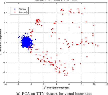
Studying the real data in telecommunicaiton networks has shown that the anoma-lies constitute a considerable amount of the population and they exhibit a group behavior as can be seen in Fig. 3.1. Therefore, the assumptions given above are valid for this problem.

Since being anomaly is not a binary property in this context, a score must be associated with each sample. This score should measure the likelihood that any given sample belongs to the anomaly class. Many researchers have proposed density measures to account for the outlierness such as LOF and OPTICS-OF [10, 11]. However, these methods generally focus on local outliers and may not achieve results as good as desired since the datasets in this thesis contain a large number of anomaly points which tend to group together. Hence, a density measure which is more robust and simpler must be devised and used.

(40)

3.3. Algorithms 29 −4 −2 0 2 4 6 8 10 12 −8 −6 −4 −2 0 2 4 6 8 1st Principal component 2 nd Principal component

Dataset: TTY, Window Size: 1500

Normal Anomaly

(a) PCA on TTY dataset for visual inspection

−2 0 2 4 6 8 10 12 14 −10 −5 0 5 10 15 20 1st Principal component 2 nd Principal component

Dataset: TTY2, Window Size: 1500

Normal Anomaly

(b) PCA on TTY2 dataset for visual inspection

Figure 3.1 Visualisation of the datasets in 2 dimensional space determined by applying PCA helps to understand the problem better. Figures 3.1(a) and 3.1(b) shows that the normal samples lie in a higher density region while anomalies reside in a sparser region.

(41)

3.3. Algorithms 30 Before going into the details of the algorithm, let us denote the dataset with D =

{xk, k = 1, . . . , M} slightly dierent than the previous subsection 3.3.1 for conve-nience. Then, let us dene the local density of a given point in the datasetD. Denition 3.3.1. Letdij be the Euclidean distance between samplexi and sample xj, where i, j ∈ {1,2, . . . , M}. From the symmetry of Euclidean distance function, dij =dji. Also, let Pi denote the set whose elements are thek-nearest neighbors of samplexi. Then, the radius of the smallest hypersphere surrounding elements of Pi is given byRi = max{dij | j ∈ Pi}. Finally, the local density for the sample xi is dened by:

Local Density=LD(xi)=

k

Volume of the hypersphere ≈ k

R2

i

In the above Def. 3.3.1, the volume of the hypersphere is approximated byR2

i assu-ming a regular sphere as this normalization factor is to be used in the same order for all samples in the dataset. Finally, the outlierness (normality) score can be dened as follows.

Denition 3.3.2. Given the local density of a sample, the density outlier score is given as

Density Outlier Score=DOS(xi)

= 1

LD(xi)

Since outliers lie in a larger sphere as their pairwise distances are relatively larger, their local densities are smaller. As a consequence, their density outlier score (DOS) gets larger compared to normal samples. However, density outlier score may suer in identifying certain anomalous objects even if they are clearly behaving oddly. This situation may arise when anomalies tend to cumulate around a certain point in space, i.e. when they form clusters themselves. Although Assumption 2 takes into account these phenomena, if the density of these clusters gets similar to those of normal samples, it breaks. Therefore, one must include another term in the nal outlier score in order to identify those ones correctly. Using Assumption 1, those objects located far away (relatively) w.r.t. the mean can be penalized. Hence, the

(42)

3.3. Algorithms 31 nal outlier score becomes:

Outlier Score=OS(xi)

=Density Outlier Score(xi)+β Distance to Mean

= 1

LD(xi)

+β×diµ

where diµ is the euclidean distance of object (sample) xi to the mean (µ) of the dataset. The variable β is controlling the penalization. Setting β = 0 would imply

that the anomality is solely based on the local density whereas any nonzeroβ implies that both assumptions are taken into account simultaneously.

Clustering based on Outlier Scores

Similar to the Naive Bayesian approach, clustering is conducted by simple threshol-ding after every data instance is associated with an outlier score. Let us denote the threshold according to which the instances are categorized asToutlier such that

c=    anomaly, if OS(xi)>Toutlier normal, otherwise

The selection of the optimal threshold is again determined through experimentation. It will be given in detail in the next chapter.

3.3.3 Ordering Points to Identify the Clustering Structure

(OPTICS)-based Approach

In this section, another density-based clustering method OPTICS [6] will be inves-tigated as well as its anomaly detection variant OPTICS-OF [10]. OPTICS simply uses the denitions of anomalies to generate an ordering of the samples in a da-taset (based on their density characteristics) rather than clustering it explicitly. In the context of this thesis, OPTICS is to be used with its variant OPTICS-OF to produce an anomaly score as have been done in the previous sections. In the way to construct a metric to evaluate samples, one should consider the denitions to be given step-by-step. These denitions are usually used for density-based cluste-ring approaches to identify samples' characteristics relative to their neighborhoods in high-dimensional feature space.

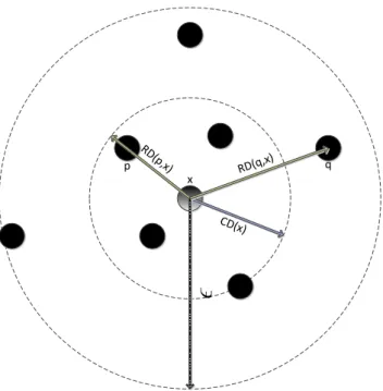
Denition 3.3.3. (-neighborhood)

The -neighborhood denes a set of samples which lie within a (hyper)sphere of radius.

(43)

3.3. Algorithms 32 r x q

ϵ

t s p v u

Figure 3.2 The -neighborhood (N(x)) constitutes of the neighbors, xi, of x which

satisfykx−xik ≤. In this gure, xi ∈N(x) ={p, q, r, s, t, u, v, x}. The sample x is by

denition in this set.

Denition 3.3.4. (directly-density-reachable)

A samplexis said to be density-reachable from another sampleqin datasetDgiven an and MinPts if

• x∈N(q), where N(q)is the set of samples in -neighborhood of q. and

• |N(q)| ≥ MinPts. This is referred to as core object condition. Denition 3.3.5. (Density-reachable)

A samplexis density-reachable from another sample q in datasetDgiven an and MinPts if there exists a chain of samples x1 = x, . . . ,xn =q such that every xi+1

is directly-density-reachable fromxi. To note, density reachability is not necessarily symmetric and only those core samples can have this symmetry.

Denition 3.3.6. (Density-connected)

A samplexis density-connected from another sampleqin dataset Dgiven anand MinPts if there exists a sampleo such that x and q are density-reachable from it.

Unlike density-reachability, densitiy connectedness is symmetric.

The above denitions can be used to conduct density-based clustering as DBSCAN does [22]. A densitycluster consists of density connected samples. Any sample in

(44)

3.3. Algorithms 33 D that does not belong to any of the existing clusters is considered as noise (not necessarily anomaly).

Although the idea in DBSCAN sorts out the clustering problem when there is noise in the dataset, it relies on the choice of parameters,MinPts which in return aect the performance of the operation. OPTICS aims at going around this pitfall by con-sidering multiple density clusters w.r.t. multiple parameters simultaneously. In order to be able to achieve this, it follows an order by which the clusters are expanded. This order imposes to choose the density-reachable object w.r.t. the smallest va-lue. Consequently, the higher density clusters are handled rst. While forming this ordering, core-distance and reachability-distance are stored and they will be utilized in the anomaly detection.

Denition 3.3.7. (Core-distance)

A samplex's core distance is dened as follows given ,MinPts. CD(x) =

 



UNDEFINED, if |N(x)|<MinPts M inP ts−distance(x), otherwise

where MinPts-distance(x) is dened as the distance between x and its MinPts' -neighbor. The core-distance can be interpreted as the minimum distance (¯) between samplexandq ∈N(x)such that xbecomes a core object w.r.t. ¯whenx satises core object condition (see Def.3.3.4). In Fig. 3.3, core-distance notion is illustrated. Denition 3.3.8. (Reachability-distance)

The reachability distance of sample q w.r.t. another sample xis dened to be:

RD(q,x) =

 



UNDEFINED, if |N(x)|<MinPts

max(CD(x), distance(q,x)), otherwise

This denition is very useful in the sense that anomalies are lying relatively remotely to such core objects. To exploit it, further denitions are necessary to be made. Additionally, to simplify the calculations all the samples will be considered as core objects [16]. Thus, denition of core-distance and reachability-distance will demand slight changes.

• Core-distance is modied to be the distance between samplexand its MinPtsth

nearest neighbor.

(45)

3.3. Algorithms 34 p x q CD(x) RD (p,x₎

ϵ

RD(q,x)

Figure 3.3 Illustration of core and reachability distances when MinPts is set to 5. The

-neighborhood (N(x)) contains more than MinPts samples implying that x is satisfying

the core object condition.

RD(x) = max(CD(q), distance(x,q)), where q is the nearest neighbor of

sample x.

Based on [10], the following will be used to compute outlier scores. Denition 3.3.9. (Local reachability density)