TEXT ANALYTICS METHODS FOR
SENTENCE-LEVEL SENTIMENT ANALYSIS
Faculty of Information Technology and Communication Sciences Master of Science thesis May 2019
ABSTRACT
Nannan Zou: Text Analytics Methods for Sentence-level Sentiment Analysis Master of Science thesis
Tampere University
Degree Programme in Electrical Engineering May 2019
Opinions have important effects on the process of decision making. With the explosion of text information on networks, sentiment analysis, which aims at predicting the opinions of people about specific entities, has become a popular tool to make sense of countless text information. There are multiple approaches for sentence-level sentiment analysis, including machine-learning methods and lexicon-based methods. In this MSc thesis we studied two typical sentiment analysis techniques – AFINN and RNTN, which are also the representation of lexicon-based and machine-learning methods, respectively.
The assumption of a lexicon-based method is that the sum of sentiment orientation of each word or phrase predicts the contextual sentiment polarity. AFINN is a word list with sentiment
strength ranging from −5 to +5, which is constructed with the inclusion of Internet slang and
obscene words. With AFINN, we extract sentiment words from sentences and sentiment scores are then assigned to these words. The sentiment of a sentence is aggregated as the sum of scores from all its words.
The Stanford Sentiment Treebank is a corpus with labeled parse trees, which provides the community with the possibility to train compositional models based on supervised machine learn-ing techniques. The labels of Stanford Sentiment Treebank involve 5 categories: negative, some-what negative, neutral, somesome-what positive and positive. Compared to the standard recursive neural network (RNN) and Matrix-Vector RNN, Recursive Neural Tensor Network (RNTN) is a more powerful composition model to compute compositional vector representations for input sen-tences. Dependent on the Stanford Sentiment Treebank, RNTN can predict the sentiment of input sentences by its computed vector representations.
With the benchmark datasets that cover diverse data sources, we carry out a thorough parison between AFINN and RNTN. Our results highlight that although RNTN is much more com-plicated than AFINN, the performance of RNTN is not better than that of AFINN. To some extent, AFINN is more simple, more generic and takes less computation resources than RNTN in senti-ment analysis.
Keywords: text mining, sentiment analysis, machine-learning methods, lexicon-based methods, AFINN, RNTN, performance assessment, hypothesis test, bootstrap, cross-validation
PREFACE
First, lots of thanks to my supervisor, Prof. Frank Emmert-Streib. During the thesis process, he created the topic, provided assistance and feedback to my research and writing. From him, I learned how to start the research and a serious attitude to my work. He is so patient and he is also one of the best professors in my life.
Second, thanks to the authors of the LATEX community and R packages. With their work, I can carry out my experiments successfully and present a beautiful thesis format. Third, thanks to the authors who provided the original datasets that are used in our ex-periments and the computational resources provided by Tampere University.
Fourth, I would like to thank my family for their encouragements to take on this study and putting up with me for the past four years.
And last but not least, I am grateful to my friend, Han Feng. During my thesis writing, I got into trouble with my life and sometimes I almost gave up the thesis. It was him who was always encouraging me to believe that the life would become better and I could make it. I also would like to thank my friend Shubo Yan for his encouragements, dumplings and help for printing. A big thank you to my favorite singer Chenyu Hua whose songs accompanied me every day and night, and all friends who supported and comforted me during this period.
Tampere, 9th May 2019
CONTENTS
List of Figures . . . v
List of Tables . . . vii
List of Symbols and Abbreviations . . . ix
1 Introduction . . . 1
2 Theoretical background . . . 4
2.1 Natural language processing . . . 4
2.2 Text mining . . . 6 2.3 Text encoding . . . 7 2.3.1 Tokenization . . . 7 2.3.2 Filtering . . . 8 2.3.3 Lemmatization . . . 8 2.3.4 Stemming . . . 9 2.3.5 Linguistic processing . . . 9
2.4 Machine learning classifiers . . . 10
2.4.1 Naive Bayes classifier . . . 10
2.4.2 Nearest Neighbor classifier . . . 10
2.4.3 Maximum Entropy . . . 11
2.4.4 Decision trees . . . 11
2.4.5 Support Vector Machines . . . 12
2.4.6 Deep learning . . . 12 2.5 Lexicon-based methods . . . 12 2.5.1 Emoticons . . . 13 2.5.2 LIWC . . . 13 2.5.3 SentiStrength . . . 14 2.5.4 SentiWordNet . . . 14 2.5.5 SenticNet . . . 15 2.5.6 Happiness Index . . . 16
3 Research methodology and materials . . . 17
3.1 Software and hardware . . . 17
3.2 A Lexicon-based method for sentiment analysis (AFINN) . . . 17
3.2.1 Construction of AFINN . . . 18
3.2.2 Sentiment prediction . . . 19
3.3 Stanford Recursive Neural Tensor Network (RNTN) . . . 20
3.3.1 Stanford Sentiment Treebank . . . 21
3.3.2 Recursive Neural Models . . . 22
3.4 Data . . . 25
3.5 Performance assessment . . . 27
3.5.1 Cross validation . . . 28
3.5.2 Bootstrap . . . 29
4 Results and discussion . . . 30
4.1 2-Class comparisons . . . 30 4.1.1 Bootstrap . . . 30 4.1.2 Cross validation . . . 35 4.2 3-Class comparisons . . . 43 4.2.1 Bootstrap . . . 43 4.2.2 Cross validation . . . 51 4.3 Discussion . . . 59 5 Conclusion . . . 62 References . . . 64
LIST OF FIGURES
2.1 A simple procedure of Text Mining [17]. . . 7 3.1 Histogram of sentiment scores for AFINN [42]. . . 19 3.2 An example of RNTN [62]. . . 21 3.3 The normalized histogram of sentiment labels at eachn-gram length [62]. . 21 3.4 Approach of computing compositional vector representations for phrases
[62]. . . 22 4.1 The LS regression model (the red line) and the diagonal model (the black
line) for the standard errors of fundamental errors of AFINN and RNTN in 2-class bootstrap. . . 32 4.2 The LS regression model (the red line) and the diagonal model (the black
line) for the fundamental errors of AFINN and RNTN in 2-class bootstrap. . 33 4.3 The LS regression model (the red line) and the diagonal model (the black
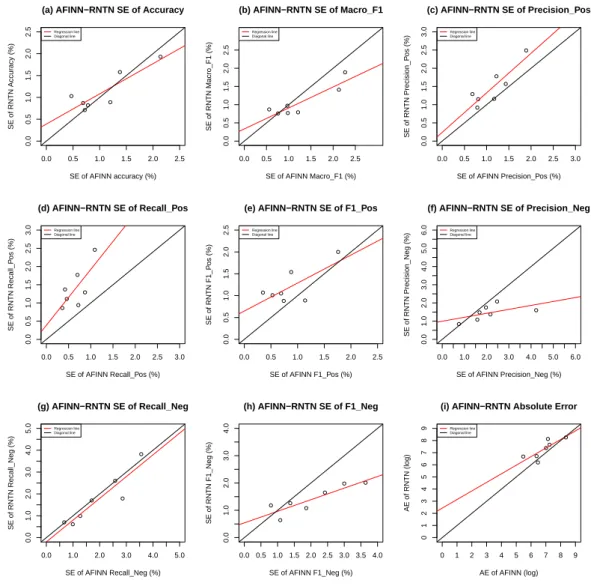
line) for the standard errors of performance assessment results of AFINN and RNTN in 2-class bootstrap. . . 35 4.4 The LS regression model (the red line) and the diagonal model (the black
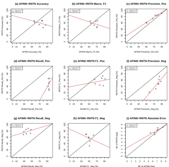
line) for the performance assessment results of AFINN and RNTN in 2-class bootstrap. . . 36 4.5 The LS regression model (the red line) and the diagonal model (the black
line) for the standard errors of fundamental errors of AFINN and RNTN in 2-class cross-validation. . . 38 4.6 The LS regression model (the red line) and the diagonal model (the black
line) for the fundamental errors of AFINN and RNTN in 2-class cross-validation. . . 39 4.7 The LS regression model (the red line) and the diagonal model (the black
line) for the standard errors of performance assessment results of AFINN and RNTN in 2-class cross-validation. . . 41 4.8 The LS regression model (the red line) and the diagonal model (the black
line) for the performance assessment results of AFINN and RNTN in 2-class cross-validation. . . 42 4.9 The LS regression model (the red line) and the diagonal model (the black
line) for the standard errors of fundamental errors of AFINN and RNTN in 3-class bootstrap. . . 44 4.10 The LS regression model (the red line) and the diagonal model (the black
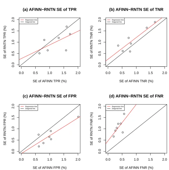
4.11 The LS regression model (the red line) and the diagonal model (the black line) for the standard errors of performance assessment results of AFINN and RNTN in 3-class bootstrap. . . 47 4.12 The LS regression model (the red line) and the diagonal model (the black
line) for the performance assessment results of AFINN and RNTN in 3-class bootstrap. . . 50 4.13 The LS regression model (the red line) and the diagonal model (the black
line) for the standard errors of fundamental errors of AFINN and RNTN in 3-class cross-validation. . . 52 4.14 The LS regression model (the red line) and the diagonal model (the black
line) for the fundamental errors of AFINN and RNTN in 3-class cross-validation. . . 53 4.15 The LS regression model (the red line) and the diagonal model (the black
line) for the standard errors of performance assessment results of AFINN and RNTN in 3-class cross-validation. . . 55 4.16 The LS regression model (the red line) and the diagonal model (the black
line) for the performance assessment results of AFINN and RNTN in 3-class cross-validation. . . 58
LIST OF TABLES
2.1 Sample emoticons and their variations [22]. . . 13
2.2 A simple example of LIWC2007 lexicon [63]. . . 14
2.3 Sample words from the lexicon of SentiStrength [65]. . . 14
2.4 The 5 top-ranked positive and negative synsets in SentiWordNet 3.0 [16]. . 15
2.5 Sample concepts with sentiment scores in SenticNet [7]. . . 15
2.6 Sample words from the lexicon of Happiness Index [6]. . . 16
3.1 An example of AFINN lexicon [42]. . . 19
3.2 Overview of our datasets for sentiment analysis. . . 27
3.3 A 3×3 confusion matrix for 3-class classification [53]. . . 27
3.4 A 2×2 confusion matrix for 2-class classification [15]. . . 28
4.1 The hypothesis test in each experiment. . . 30
4.2 The fundamental errors of 2-class bootstrap with seven datasets for senti-ment analysis, classifier=AFINN. . . 31
4.3 The fundamental errors of 2-class bootstrap with seven datasets for senti-ment analysis, classifier=RNTN. . . 31
4.4 The hypothesis testing results for Figure 4.1. . . 31
4.5 The hypothesis testing results for Figure 4.2 . . . 32
4.6 The performance assessment results of 2-class bootstrap with seven datasets for sentiment analysis, classifier=AFINN. . . 33
4.7 The performance assessment results of 2-class bootstrap with seven datasets for sentiment analysis, classifier=RNTN. . . 34
4.8 The hypothesis testing results for Figure 4.3. . . 34
4.9 The hypothesis testing results for Figure 4.4. . . 36
4.10 The fundamental errors of 2-class cross-validation with seven datasets for sentiment analysis, classifier=AFINN. . . 37
4.11 The fundamental errors of 2-class cross-validation with seven datasets for sentiment analysis, classifier=RNTN. . . 37
4.12 The hypothesis testing results for Figure 4.5. . . 37
4.13 The hypothesis testing results for Figure 4.6. . . 38
4.14 The performance assessment results of 2-class cross-validation with seven datasets for sentiment analysis, classifier=AFINN. . . 39
4.15 The performance assessment results of 2-class cross-validation with seven datasets for sentiment analysis, classifier=RNTN. . . 40
4.16 The hypothesis testing results for Figure 4.7. . . 40
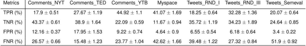
4.18 The fundamental errors of 3-class bootstrap with seven datasets for senti-ment analysis, classifier=AFINN. . . 43 4.19 The fundamental errors of 3-class bootstrap with seven datasets for
senti-ment analysis, classifier=RNTN. . . 43 4.20 The hypothesis testing results for Figure 4.9. . . 45 4.21 The hypothesis testing results for Figure 4.10. . . 45 4.22 The performance assessment results of 3-class bootstrap with seven datasets
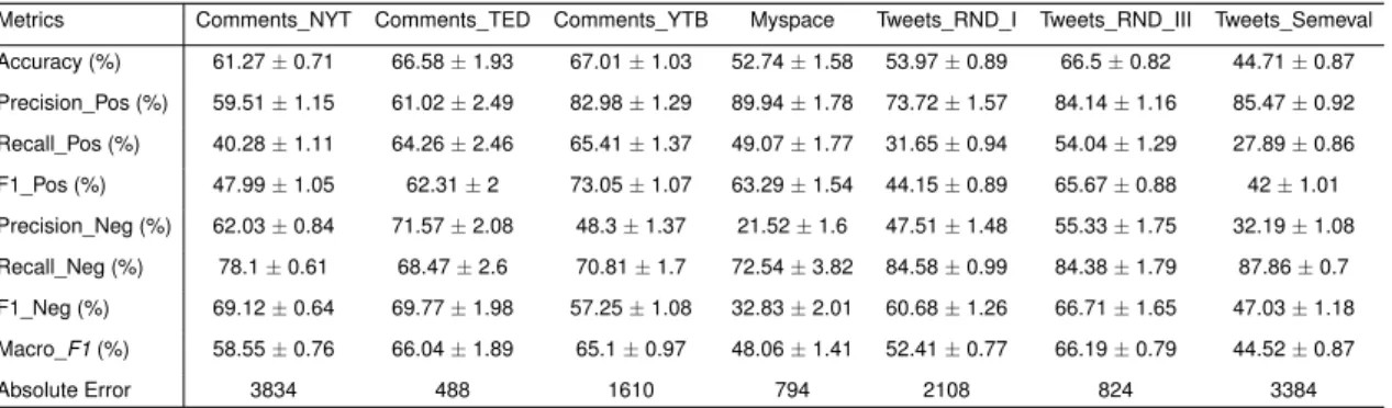
for sentiment analysis, classifier=AFINN. . . 48 4.23 The performance assessment results of 3-class bootstrap with seven datasets
for sentiment analysis, classifier=RNTN. . . 48 4.24 The hypothesis testing results for Figure 4.11. . . 49 4.25 The hypothesis testing results for Figure 4.12. . . 49 4.26 The fundamental errors of 3-class cross-validation with seven datasets for
sentiment analysis, classifier=AFINN. . . 51 4.27 The fundamental errors of 3-class cross-validation with seven datasets for
sentiment analysis, classifier=RNTN. . . 51 4.28 The hypothesis testing results for Figure 4.13. . . 54 4.29 The hypothesis testing results for Figure 4.14. . . 54 4.30 The performance assessment results of 3-class cross-validation with seven
datasets for sentiment analysis, classifier=AFINN. . . 56 4.31 The performance assessment results of 3-class cross-validation with seven
datasets for sentiment analysis, classifier=RNTN. . . 56 4.32 The hypothesis testing results for Figure 4.15. . . 57 4.33 The hypothesis testing results for Figure 4.16. . . 57
LIST OF SYMBOLS AND ABBREVIATIONS
A accuracy
AFINN a lexicon-based method for sentiment analysis
AI artificial intelligence
AMT Amazon Mechanical Turk
ANEW Affective Norms for English Words
CK Cohen’s Kappa
Dt data set
D data set
E error function
F1 the harmonic average of precision and recall
f NN function
FNeR false neutral ratio
FNR false negative ratio
FPR false positive ratio
h the output of a tensor product
IVR Interactive Voice Response
kNN k-nearest neighbor classification
λ a weight vector in Maximum Entropy
LIWC a dictionary-based analysis tool
LOOCV leave-one-out cross validation
Macro-F1 averageF1scores over all classes
MaxEnt maximum entropy
MV-RNN matrix-vector recursive neural network
Neg negative class
Neu neutral class
NLP natural nanguage processing
NYT New York Times
p the parent vector
P(c) the prior probability of class
PM E the conditional probability in Maximum Entropy
P(X|c) the probability of predictor given class
P(X) the prior probability of predictor
P precision of a class
POS part-of-speech
Pos positive class
R recall of a class
RNN recursive neural network
RNTN Stanford Recursive Neural Tensor Network
SE standard error
SVM support vector machine
TCSC Tampere Center for Scientific Computing
TED a media organization
TNR true negative ratio
TPR true positive ratio
U a uniform distribution
V matrix of each tensor slice
Ws the sentiment classification matrix
W weight of neuron
WSD word sense disambiguation
1 INTRODUCTION
Opinions from ordinary people and experts always have significant influences on the pro-cess of decision making. Finding out "What others think" forms an important part for most of us to gather information. Even before the World Wide Web, we always asked friends to explain their opinions about political events, requested colleagues for recommendation letters, or consulted a shopping-guide to determine what dishwasher to purchase [47]. As the Internet and the Web became more and more widespread, it is now possible for people to search for various views. For instance, in two surveys of more than 2000 Amer-ican adults, 32% have posted ratings regarding a product or service, and more than 73% report that online comments had important effects on their purchase [47]. Similarly, ac-cording to another survey of over 2500 American adults, approximate 30% have the need for political information [47]. However, the problem of overwhelming and confusing on-line information leads to a rapidly increasing demand for better information-understanding system.
Data science is a novel discipline that emphasizes on extracting implicit, nontrivial and potentially meaningful information from data [14]. The basic motivation behind data sci-ence is that valuable information is contained in these large databases but concealed within the mass of uninteresting data. Data science combines techniques and theories drawn from many fields like statistics, mathematics, and computer science. Primarily, predictive causal analytics, prescriptive analytics and machine learning are used to make decisions and predictions in data science [25].
Mining information from large databases has been recognized as an important topic in research, and it also provides a great opportunity of revenues for many industrial com-panies. The applications of extracted information consist of decision making, information management, process control, query processing and etc. Moreover, some emerging ap-plications in information delivery services, such as online services, also use a variety of information mining approaches to improve their work [8].
Text mining is known as information extraction from textual database [27]. It is the ex-traction of novel and interesting knowledge from diverse written resources. However, text mining is different from what users usually do in web search [24]. In web search, the pur-pose is to look for something that is already aware of and has been written by someone else. The only difficulty is to select what you need and push aside all the materials that are not relevant. In text mining, user are trying to discover something that is non-trivial and so could not have been yet written down [24].
Due to such a fact, sentiment analysis, which aims at predicting the opinions of authors about specific entities, is a currently hot research area in text mining. Explosive social media sites, such as Twitter, Facebook, blogs, user forums and message boards, provide an extremely convenient way for individuals and organizations to monitor their reputation and get real-time feedback [19]. Nevertheless, since privately and publicly available in-formation is constantly growing over Internet, it is tricky for a human reader to identify relevant sites and accurately summarize the opinions within them [36]. Furthermore, it is difficult for people to produce consistent results with a large amount of information, due to their physical and mental limitations [36]. Thus, sentiment analysis has become a popular tool to make sense of countless text information.
Nowadays, there is a considerable number of applications of sentiment analysis. Over 7,000 articles have been written about such a technique, and various startups are de-veloping solutions and packages to analyze and monitor sentiments on social networks [19]. Many online merchants enable their customers to review the products they have purchased, and keep track customer opinions with the analysis of their reviews [28]. In finance, financial investors make use of sentiment analysis to discover public moods on the market and indicate analytical perspective [5, 43]. Another successful application is in politics, where the analysis of political sentiment closely relates to the candidates’ political positions [66]. In some ways, it can reflect the election result.
Sentiment analysis can be categorized into three specific groups: document-level senti-ment analysis, sentence-level sentisenti-ment analysis, and aspect-based sentisenti-ment analysis [19]. Document-level sentiment analysis is the simplest form of sentiment analysis and its assumption is that the author expresses an opinion on one major object in this docu-ment. A document can be segmented into multiple sentences; therefore, sentence-level sentiment analysis means obtaining the sentiment of an individual sentence. Neverthe-less, not all the sentences contain opinions and present sentiment polarity [69]. Because objective sentences have no help to infer the polarity, only subjective sentences deserves further analyzing. In other words, sentence-level sentiment analysis is also known as po-larity classification. One entity usually have numerous attributes and people often have different opinions about each of these attributes. Thus, aspect-based sentiment analysis provides the possibility to detect all the sentiments within the given entity. Due to the particular short sentences that people prefer to use on social networks, in this thesis we mainly focus on the sentence-level sentiment analysis [19].
In recent years, a huge amount of approaches have been proposed for sentence-level sentiment analysis. To achieve state-of-the-art performance, recent methods mostly adopt machine learning algorithms or lexical-based algorithms. With advances in com-puter technology, machine learning is an application of artificial intelligence (AI) which is undergoing intense development. It denotes methods which provide computers with the ability to learn and improve automatically without human intervention or assistance [1]. Machine learning techniques usually include two categories: supervised learning and unsupervised learning [1].
Supervised learning, where the desired outputs have been labeled, aims to learn a func-tion that best approximates the relafunc-tionship between inputs and outputs. In contrast, the goal of unsupervised learning, without labeled outputs, is to automatically identify the natural structure in data. Machine learning has been applied successfully on many fields, for instance, it has demonstrated outstanding performance in bioinformatics [4], natural language processing [10], computer vision [55], and data mining [67]. Moreover, machine learning methods are currently active and showing significant performances on sentiment analysis tasks. These techniques are completely prior-knowledge-free, and they attempt to learn an end-to-end mapping between sentences and sentiment polarities. The most common machine learning methods in sentiment analysis include Neural Networks, Naive Bayes classification, Support Vector Machines and Maximum Entropy classification [46]. However, lexicon-based methods need strong prior information. The lexicon-based meth-ods use a predefined dictionary in which each word corresponds to a specific sentiment. The sentiment dictionary plays a key role in sentiment analysis tasks. Mostly, subjective sentences can be separated into sentiment terms (words or phrases) which convey pos-itive or negative sentiment polarities [50]. The identification of polarities for such terms would help in better inferring sentiment of the whole sentence. Nevertheless, these ap-proaches require diverse predefined dictionaries to adapt to varying contexts. For exam-ple, PANAS-t was proposed to analyze sentiments based on a well-established psycho-metric scale [23], whereas Linguistic Inquiry and Word Count (LIWC) was proposed to measure more formal psychological words [63].
Since the state-of-the-art performance has not been clearly confirmed, any popular ma-chine learning or lexicon-based approaches are acceptable by the research community to measure sentiments. Nevertheless, we are aware of little about relative efficiency and performance of the two different approaches. In other words, many recently proposed techniques are widely deployed for developing applications without deeper comparing their efficiency in distinct contexts with each other [19]. Therefore, it is necessary to con-duct a thorough comparison of machine learning and lexicon-based sentiment analysis approaches across multiple datasets.
In this thesis, we introduce various approaches for sentence-level sentiment analysis, including machine-learning methods and lexicon-based methods. Additionally, we study two typical sentiment analysis techniques: AFINN and RNTN. With the benchmark datasets that cover diverse data sources, we also carry out a thorough comparison between AFINN and RNTN.
The remainder of this thesis is organized as follows. In Chapter 2, we briefly review the-oretical background. In Chapter 3, we describe the software and hardware resources, sentiment analysis techniques that we compared, datasets and performance assess-ment approaches. Chapter 4 summarizes our results and analysis. Finally, Chapter 5 concludes the thesis and presents direction for future work.
2 THEORETICAL BACKGROUND
In this chapter, we shall first discuss natural language processing, text mining and text en-coding that forms the basic components of sentiment analysis. Furthermore, background and existing related work on sentence-level sentiment analysis are briefly reviewed.
2.1 Natural language processing
Natural Language Processing (NLP) focuses on the field that aids computers to under-stand and manipulate the human’s natural language. NLP researchers are interested in exploring how humans understand and communicate with natural language, and then the computer systems can use these techniques to manipulate natural languages to solve target problems. NLP combines the fields of linguistics, electrical and electronic engi-neering, robotics, statistics, psychology, artificial intelligence, and computer sciences [9]. NLP can perform outstanding in a number of common applications, such as language translation (e.g. Google Translate), Interactive Voice Response (IVR), personal assistant (e.g. Siri), and speech recognition.
The core idea behind NLP is natural language understanding. For computers, there are three principal problems in understanding humans’ natural languages: thought proce-dures, the representation and meaning of the linguistic input, and the world knowledge [9]. When a text has been provided, the NLP program will utilize algorithms to decide the morphological structure and nature at the word level. Then, it will try to extract mean-ing associated with the whole sentence and collect the essential information. Finally, the program will consider the context or the overall domain of the given text. Sometimes, the NLP program may fail to correctly understand the meaning of a sentence, since the given context has a significant effect on the connotation of words or sentences.
A program that actually "understands" natural language is difficult to be determined in the NLP research. All we can actually test is whether a program appears to understand humans’ language by successfully completing its task. The Turing test (q.v.), proposed by Turing, has been the classical model [9]. In this test, the NLP program has to be undis-tinguishable from a human when both answer arbitrary interrogation by a human over a terminal. A growing concern in NLP is developing more sensitive models of evaluation that can measure progress. The common method is to carry out evaluation tests within restricted domains to examine specific capabilities. For instance, statistical measures
can be computed relied on the set of human-generated questions collected in protocols (q.v.) that use another human to simulate the program.
Actually, the pervasive ambiguity is the major problem in processing natural language. Several common ambiguity are introduced in the following:
• Simple lexical ambiguity. For example, "bank" can be a noun (the financial insti-tution) or a verb (to tip laterally).
• Structural or syntactic ambiguity. For example, in the sentence "Jack helped the woman with a wheelchair", the wheelchair might be utilized for the help or might be used by the woman being helped.
• Semantic ambiguity. For example, the word "make" has more than 10 different meanings in any dictionary.
• Pragmatic ambiguity. For example, "Could you pass the water to me?" may be a request to pass the water or a yes/no question.
• Referential ambiguity. For example, "Jorge talked with Frank in Starbucks. He looked bad . . . ," it is not clear who looks bad, even the remainder of the sentence might suggest a correct answer.
The history of NLP could be divided into four phases [30] with different concerns and styles. The first phase emerged from the need of Machine Translation in the 1940s [30]. Initially, machine translation mainly focused on English and Russian. Gradually, other languages such as Chinese also became popular in the 1960s. However, machine trans-lation had little development during 1966 as the research of this field almost died at that time [56].
Since the need of Artificial Intelligence (AI) emerged, NLP acquired a new life in the 1980s [30]. This phase focused on meaning representation and gave more attention to world knowledge. LUNAR, developed by W.A woods in 1978, is a pioneering work of the question-answering systems influenced by AI [56]. The Yale group early recognized the need to explore the humans’ goals if the NLP techniques wanted to completely un-derstand the natural language. Thus, this phase also emphasized on both surface and underlying meanings of the language.
In the period of 1990s, NLP started to grow quickly. This trend was stimulated by the development of grammars, tools and practical resources [30]. For example, word sense disambiguation and statistically colored NLP had become the most striking feature of this decade. Additionally, NLP techniques of this phase involved other essential topics, such as semantic classification, information extraction, statistical language processing, and automatic summarizing [56].
Currently, everyone expects the machine to think and talk like humans, and the Natural Language Processing is the only method which can help us to achieve this goal. Many talking machines named Chatbot, such as Alexa developed by Amazon, can manage complicated interactions with human beings and process the streamlined business [56].
Particularly, the integration with Machine Learning and Deep Learning greatly expands the capabilities of NLP technology. Nowadays NLP techniques can be used to handle many different areas, such as health care, sentiment analysis, cognitive analytics, spam detection, human resources and conversational framework.
Text mining is the process to discover and extract useful and nontrivial information from unstructured text. This process involves the disciplines of information retrieval, text classi-fication and clustering, and event extraction. NLP is the technique that attempts to explore the patterns to represent a full meaning of the unstructured text. NLP typically utilizes syntax techniques such as lemmatization, morphological segmentation, word segmenta-tion, part-of-speech tagging, parsing, sentence breaking and stemming; semantics such as named entity recognition, word sense disambiguation and natural language genera-tion; grammatical structure such as noun phrase, prepositional phrase, and dependency relations [31].
Modern NLP includes machine learning, machine translation, speech recognition, and machine text reading. Combining these branches together means that AI has the ability to acquire real knowledge from the world, not just learning the experience from humans. In the future, computers will have the capability of gaining information online and learn from it. With the continuous research, NLP will reach at a human level of understanding and awareness [35].
2.2 Text mining
Text mining is a young subject which focuses on detecting useful patterns from large database [3]. It combines the fields of information retrieval, data mining, machine learn-ing, statistics and computational linguistics together, and extracts new pieces of knowl-edge from textual data. Although the sources of new knowlknowl-edge are diverse, unstructured texts, such as webpages, e-mail messages, and many business documents etc., are still the largest readily accessible source of discovery [27]. Thus, the obvious distinction be-tween text mining and regular data mining is that the patterns of data mining are extracted from structured database of facts [26].
With electronic files becoming the main method of sorting, storing and accessing written information, managing electronic information is changing the world greatly. Many other fields, like manufacturing, education, business, health care and government, can ben-efit from text-mining techniques. As a result, text mining technology and solutions are considered to have a high potential worth.
The main problem of text mining is machine intelligence [17]. It is easy for humans to identify and employ linguistic patterns to text and overcome obstacles like spelling variations, a slang and contextual meaning, while computers cannot manage them easily. On the other hand, humans are not able to handle texts in large volumes or at high speeds [17], though they are capable of comprehending unstructured data. Therefore,
creating a technique with both a computer’s speed and accuracy and a human’s linguistic capabilities is the key to text mining.
Figure 2.1. A simple procedure of Text Mining [17].
Figure 2.1 exhibits a simple example of the text mining procedure. It starts with a group of documents, and then checks the format and word lists of the retrieved particular doc-ument. After that, it implements text analysis, repeating a combinations of techniques, such as information extraction, clustering and summarization, to extract the targeted in-formation. Finally, the management information system can process the resulting infor-mation to generate knowledge for its users.
In order to narrow the gap between humans and computers, various technologies that teach computers to analyze and understand natural languages have been produced. They consist of topic tracking, categorization, information extraction, information visu-alization, summarization, question answering, clustering, and concept linkage [17]. With these techniques, text mining has been demonstrated to be helpful in telecommunica-tions, biomedical engineering, climate data, and geospatial data sets.
2.3 Text encoding
Preprocessing the text files and storing the contents in a data structure is a necessary step for text mining, which is convenient for further processing. Although exploring the syntactic structure and semantics is a key point in some methods, many text mining techniques rely on the concept that a set of words can describe a text document (bag-of-words representation). Due to the importance of bag-(bag-of-words representation, we will briefly describe how it can be obtained in the following.
2.3.1 Tokenization
The tokenization step is necessary to obtain all contained words for a given sentence. A token is a unit of text that is meaningful for analysis, such as a phrase or a word. Tokenization removes all punctuation marks and replaces other characters with white spaces, and then splits a text document into tokens. For text mining, it is easier and more
effective to use the specific tidy text format which is defined as a table with one-token-per-row [60]. In this one-token-per-one-token-per-row structure, the token can be a single word, an n-gram, a sentence or a paragraph. This tidy-text structure is then used for further processing. For example, we have a sentence "Because I could not stop f or Death". The process of tokenization needs to break the text into individual tokens "because", "i", "could", "not", "stop", "f or", "death". For another example, the phrases "new york university", right
direction, andgreen gascan also be considered as tokens.
2.3.2 Filtering
Filtering approaches can filter words from the tidy text structure and thereby from the text document. A well known filtering approach is the removal of stop words [57]. Stop words, such as articles, conjunctions, prepositions etc., represent the items bearing little or no information of the contents. Moreover, words occurring extremely often are likely to bear-ing little knowledge, and also words occurrbear-ing very seldom can be said to be no statistical relevance. Thus, all of these words belong to stop words. Stop-word filtering relies on the concept that removing non-discriminative words decreases the feature space of the classifier and assists them to generate more correct results [61]. For this reason, a stop dictionary includes the words that should be removed in the bag-of-words representation procedure. Although a set of general words, likeandandor, can be seen as stop words in almost all cases, words of the stop dictionary are dependent in languages and tasks.
2.3.3 Lemmatization
For many applications of text mining, lemmatization is a significant preprocessing step. It is also extensively applied in NLP and other domains related to linguistics [49]. Lemma-tization attempts to replace nouns with the singular form and verb forms with the infinite tense. In other words, lemmatization always looks for a transformation which can be ap-plied to a word to obtain its normalized form. The lemmatization methods are similar to word stemming, except that lemmatization only requires to find the normalized form of a word but not to generate the word stem [49].
For example, the normalized form of the wordsworking,works,workediswork; and the word stem of them is alsowork. In this context, lemmatization is equal to word stemming. However, sometimes the normalized form is different with the stem of the word [49]. For instance, the words computes, computing, computed would change to the normalized
2.3.4 Stemming
Generally, the morphological variants of words express the similar semantic meaning, and it consumes much time if each word form is considered different. Hence, it is essential to distinguish every word form with its basic form [29]. Stemming is also a preprocessing step in text-mining applications. It attempts to retrieve the base forms of words, i.e. re-move the ’s’ from nouns, the ’ed’ from verbs, or other affixes. In a word, stemming means a process to normalize all words that have the same stem to a basic form [37].
Stemming:
introduction,introducing,introduces–introduc
walked,walking,walks–walk
As explained in Lemmatization part, lemmatization requires to find the normalized form of a word (examples are showed in Lemmatization part). But stemming works by cutting off the common prefixes and suffixes of the word. This indiscriminate cutting offers limitations in some occasions. For example, the stem word of studieswould be studi which is not so meaningful for our analysis. However, a lemma word is always the base form of all its inflectional forms. For the same examplestudies, its lemma word isstudy.
2.3.5 Linguistic processing
In addition to basic text-mining preprocessing, usually linguistic processing methods are also utilized to explore more information about text. For this reason, some frequently applied approaches are introduced in the following.
Part of speech (POS) is the conventional term that classifies words in a language [58]. The grammatical property of a word is the primary criteria for part-of-speech classifica-tion. In text mining, POS tagging is usually used to determine the part-of-speech tag, such as verb, noun, and adjective, for each item.
The textual unit of adjacent tokens is named as chunk [18], and text chunking means grouping an unstructured sequence of adjacent text units in a piece of text. Each chunk includes a set of adjacent words which are mutually linked through dependency chains of some specifiable kinds [18].
Human language is ambiguous and many words bear different interpretation based on the context. Word sense disambiguation (WSD) is a technique that attempts to recognize the interpretation of single word or phrase in the context [41]. For example, the word
bank clearly denotes meanings: a financial institution that accepts deposits or the slope beside a body of water. Although WSD causes a more complex dictionary, the core idea of considering many semantics of a term is close to human comprehension.
Parsing, also known as syntactic analysis, refers to the procedure that analyzes sentence structure and generates a full parse tree of a sentence [38]. With parsing, the relation
between every word and all the others can be easily explored.
2.4 Machine learning classifiers
In this section, we briefly review six machine-learning classifiers [11, 21, 34, 51, 54, 59] which are extensively applied in the field of sentiment analysis.
2.4.1 Naive Bayes classifier
The Naive Bayes classifier is dependent on the Bayes theorem with an assumption of independent predictors [54]. Despite its simplicity, Naive Bayes classifier works well on sentiment analysis. With Bayesian theorem, we can calculate posterior probabilityP(c|X) fromP(c),P(X)andP(X|c)[54]:
P(c|x) = P(x|c)P(c)
P(x) (2.1)
P(c|X) =P(x1|c)×P(x2|c)× · · · ×P(xn|c)×P(c) (2.2)
whereP(X)is the prior probability of predictor,P(X|c)is the probability of predictor given class, andP(c)is the prior probability of class [54].
Naive Bayes classifier is simple and fast to classify the target data and it also performs outstanding in multiclass classification. Especially, Naive Bayes classifier needs less training data and performs better compared to other classifiers when holding independent assumption. However, its assumption also gives an obvious limitation, where indepen-dent predictors are almost impossible in real life.
2.4.2 Nearest Neighbor classifier
In text mining, the sentiment of the given sentence may be predicted from the sentiments of other similar sentences. Thus, this method is called as nearest neighbor classifier, wherek-nearest neighbor classification (kNN) is the most frequently useful one [11].kNN includes a training dataset of both positive and negative classes, and a target sentence is classified by computing the distance to theknearest points and assigning the label of the majority [11]. To find out the best k, a cross validation method is often carried out. We generally create a list ofkvarying among some range and then the testing accuracy is given based on the validation set. Finally, a graphkvsaccuracyis plotted, and we can determine the bestkamong the range using the plot.
computational effort during classification. In another term, it is not practical enough and takes much time to test the data, where we tend to have fast testing to have real-time results.
2.4.3 Maximum Entropy
Maximum Entropy (MaxEnt) principle arises in statistical mechanics. Unlike Naive Bayes, MaxEnt has no assumptions of independence for its attributes. To model a given data set, it indicates that the most appropriate distribution is the one with highest entropy among all those satisfying the constrains of prior knowledge [21]. Because maximizing entropy minimizes the amount of prior information built into the distribution. The MaxEnt can be represented as the following:
PM E(c|d, λ) = exp[∑ iλifi(c, d)] ∑ cexp[ ∑ iλifi(c, d)] (2.3)
Herecmeans the class, d describes the sentence, andλindicates a weight vector. The weight vectors are optimized by numerical optimization ofλto maximize the conditional probability [21].
In text mining practice, the features to model MaxEnt are linguistically simple, but yet outperform many of learning algorithms under similar circumstances. The major disad-vantage is that the exact maximum entropy solution does not exist in some cases, where the probability distribution may lead to poor testing accuracy [52].
2.4.4 Decision trees
Decision tree classifier, which involves decision nodes and leaf nodes, yields a final deci-sion by repetitively dividing a dataset into gradually smaller subsets [51]. A decideci-sion node includes two or more branches, while a leaf node states a decision. Once the decision tree has been constructed, classifying a sentence is straightforward. Hence, constructing an optimal decision tree is the key aspect in the decision tree classifier. LetDt be the training dataset and the attributeti is selected. Then Dt is split into two subsets. The subset Dt+i contains the sentences includingti, and the subset Dt−i includes the sen-tences withoutti. This process is recursively applied toDt+i andDt−i until all sentences in a subset are classified as the same class.
Decision trees can easily handle irrelevant attributes and missing data, and they are also quite fast at testing time [51]. Nevertheless, the disadvantage is that the final decision is determined only on relatively few features in sentiment analysis. And also, sometimes they may not find the best tree in real world.
2.4.5 Support Vector Machines
The Support Vector Machine (SVM) means a discriminative classifier which attempts to find a separating hyperplane that distinctly classifies the data points in ann-dimensional space [59]. In other terms, SVMs output an optimal decision surface that categorizes new samples dependent on labeled training data. In sentiment analysis, the SVM classifier decides a hyperplane that is settled between the positive and negative categories of the dataset, where the margin is particularly maximized.
The learning of SVMs is almost regardless of the dimensionality of its feature space. Because feature selection is rarely required in SVM, SVM classifier is particularly suitable for text classification which usually involves a large amount of features. In addition, the kernel function does not have an important effect on the performance of text classification, since kernels are subject to overfitting [27].
2.4.6 Deep learning
In representation learning, the raw data is fed into a computer and the computer would au-tomatically explore the needed representations for classification or detection [34]. Deep learning classifiers belong to representation learning approaches, which involve multiple levels of representation. As the non-linear modules of deep learning transform the repre-sentation between different levels, the classifier will learn quite complex functions during this process. For sentiment classification in text, the features that are significant for iden-tification are amplified and the irrelevant parameters are suppressed by deeper layers of representation. Particularly, deep learning can use their purposed learning process to learn these layers of features, instead of designed by human engineers [34].
In recent years, deep learning has demonstrated outstanding performance in solving problems. It shows great capability in discovering intricate patterns for high-dimensional data, and it has been widely used in science, business and government [34]. However, there are a few challenges that have to be tackled to develop it. First, large amounts of data are required to train deep learning algorithms – as they learn progressively. More-over, data availability for some sectors may be sparse and thus hamper deep learning in practice. Additionally, the high performing graphics processing units of deep learning require and consume a lot of power and are thereby a costly affair.
2.5 Lexicon-based methods
In this part, we briefly introduce six Lexicon-based approaches [7, 12, 16, 22, 63, 65] that are widely applied in the field of sentiment analysis.
2.5.1 Emoticons
Recently, Emoticons have become increasingly popular. Detecting the emoticons con-tained in the sentences is the simplest way for sentiment classification [22]. Because emoticons can represent happy or sad feelings, a set of common emoticons are utilized to extract polarity, such as exhibited in Table 2.1. This table consists of most popular emoticons and also their variations, which express positive, negative, and neutral polar-ities. If some sentences have more than one emoticon, then the polarity is determined with the first appeared emoticon in the text [22]. However, compared to total subjective sentences, the rate of online-social-network texts which contained at least one emoti-con is less than 10% [22]. Hence, emotiemoti-cons are usually used in combination with other methods for sentiment analysis.
Table 2.1. Sample emoticons and their variations [22].
Polarity Positive Negative Neutral
Symbols
:) :] :} :o) :o] :o} :-] :-) :-} =) =] =} =^] =^) =^} :B :-D :-B :^D :^B =B =^B =^D :’) :’] :’} =’) =’] =’} <3 ^.^^-^^_^^^:* =* :-* ;) ;] ;} :-p :-P :-b :^p :^P :^b =P =p \o\/o/ :P :p :b =b =^p =^P =^b \o/ D: D= D-: D^: D^= :( :[ :{ :o( :o[ :^( :^[ :^{ =^( =^{ >=( >=[ >={ >=( >:-{ >:-[ >:-( >=^[ >:-( :-[ :-( =( =[ ={ =^[ >:-=( >=[ >=^( :’( :’[ :’{ =’{ =’( =’[ =\:\ =/ :/ o.O O_o Oo =$ :$ :-{ >:-{ >=^{ :o{ :| =| :-| >.<><>_<:o :0 =O :@ =@ :^o :^@ -.--.-’ -_- -_-’ :x =X :# =# :-x :-@ :-# :^x :^#
2.5.2 LIWC
LIWC is a dictionary-based analysis tool, evaluating emotional, cognitive, and structural items of a given sentence [63]. Besides negative and positive categories, LIWC also detects other classes of sentiment. For instance, the term "agree" can be categorized into six word groups: affective, assent, positive feeling, positive emotion, and cognitive process. The LIWC2007 version contains labels for 100 word categories and more than 4500 English words, and Table 2.2 lists a simple example of LIWC2007 lexicon [63]. Currently, LIWC provides a commercial software and optimization option which allows users to create customized dictionaries rather than the standard ones. The LIWC soft-ware is accessible athttp://www.liwc.net/.
Table 2.2.A simple example of LIWC2007 lexicon [63].
Category Affective process Cognitive process Perceptual process
Examples
happy, cried, abandon, love, nice, sweet, hurt, ugly, nasty,
worried, fearful, nervous, hate, kill, annoyed, crying, grief, sad
cause, know, ought, think, know, consider, because, effect, hence
observing, heard, feeling, view, saw, seen,
listen, hearing, feels, touch
2.5.3 SentiStrength
The core idea of SentiStrength depends on the list of words from the LIWC lexicon. The authors added some new features, including a set of positive and negative words, the words to weaken (e.g., "a bit") or strengthen (e.g., "too") sentiments, emoticons, and re-peated punctuation (e.g., "Good!!!!") to strengthen sentiments, to expand the baseline for the online-social-network context [65]. In the experiments, the authors evaluated six dif-ferent datasets from Web 2.0: MySpace, BBC Forum, Twitter, Digg, YouTube Comments, and Runners World Forum [65]. Now, the authors also provides a useful tool to produce almost state-of-the-art results. Table 2.3 illustrates some sample words from the lexicon of SentiStrength.
Table 2.3. Sample words from the lexicon of SentiStrength [65].
List Name Sentiment word list Booster word list Idiom list Negation word list Emoticon word list Sample Word and Score Awful (-4) Blissful (+5) Slightly (-1) Extremely (+2) Shocker horror (-2) Whats good (+2) Cant (-) Never (-) :’( (-1) :-D (+1)
2.5.4 SentiWordNet
SentiWordNet relies on an English lexicon named WordNet. WordNet classifies nouns, verbs, adjectives and other grammatical groups into synsets [16]. The SentiWordNet using three values with synsets to state the polarity of the sentence: negative, positive, and neutral. The values are in the range of [0, 1] and the total sum is 1 [16]. For example, we have a given synset s = [bad, wicked, terrible], and then SentiWordNet will score negative sentiment with 0.850, positive sentiment with 0.0, and neutral sentiment with 0.150, respectively.
Generally, scores from neutral sentiment have no effect on final sentiment decision. If the average positive score of all associated synsets of a target sentence is higher than that of the negative score, the polarity would be considered to be positive. Table 2.4 lists the 5 top-ranked positive and negative synsets in SentiWordNet 3.0.
Table 2.4. The 5 top-ranked positive and negative synsets in SentiWordNet 3.0 [16]. Rank 1 2 3 4 5 Positive good#n#2 goodness#n#2 better_off#a#1 divine#a#6 elysian#a#2 inspired#a#1 good_enough#a#1 solid#a#1
Negative abject#a#2 deplorable#a#1
distressing#a#2 lamentable#a#1 pitiful#a#2 sad#a#3 sorry#a#2 bad#a#10 unfit#a#3 unsound#a#5 scrimy#a#1 cheapjack#a#1 shoddy#a#1 tawdry#a#2
2.5.5 SenticNet
SenticNet is a tool extensively utilized in opinion mining, and its goal is to infer the polarity at a semantic level instead of the syntactic level [7]. SenticNet utilizes NLP approaches to create a polarity for almost 14000 concepts [7] which are defined as common sense – obvious things we normally know and usually leave unstated . For example, suppose that a given sentence "Great, it is Friday evening" is ready for sentiment classification, Sen-ticNet first identifies concepts, which are "great" and "Friday evening" in this task. Then it produces sentiment score, between the values of -1 and 1, to every concept. In this task, "great" gets +0.383 and "Friday evening" gets +0.228, thereby the final sentiment score +0.3055 which is the average of the total values.
The authors of SenticNet evaluated it with the data of patients’ opinions about the National Health Service in England and posts with over 130 moods from LiveJournal blogs [7]. Table 2.5 exhibits some sample concepts with sentiment scores in SenticNet.
Table 2.5. Sample concepts with sentiment scores in SenticNet [7].
Concept Sentiment Score Concept Sentiment Score
Want degree 0.020 A lot +0.970
Child play 0.023 A way of +0.303
Grow up 0.290 Abandon -0.858
Birthday cake 0.292 Abash -0.130
Enough food 0.580 Abhor -0.376
Wood spoon -0.023 Able use +0.941
Death row -0.290 Abhorrent -0.396
2.5.6 Happiness Index
The method of Happiness Index bases on the Affective Norms for English Words (ANEW) [12]. ANEW involves a list of 1034 unique words which are widely associated with their valence (ranging from pleasant to unpleasant), arousal (ranging from calm to excited)), and dominance [6]. Osgood’s [44] seminal work indicates that these three dimensions can account for the variance in emotional assessments. Happiness Index indicating the quantity of happiness present in the message by giving scores for given terms between the values of 1 and 9. To increase the accuracy, the authors computed the appearing frequency of ANEW words in the sentences and calculated a weighted valence. When the weighted valence is evaluated on the song titles, song lyrics, and micro-blogs, the authors explored that the happiness value had decreased from 1961 to 2007 for song lyrics, while the value for blogs had increased during the same time [12].
To adapt this method for polarity classification, sentence that is categorized with Happi-ness Index in the spanning of [1, 5) is considered to be negative and in the spanning of [5, 9] is considered to be positive [12]. Table 2.6 presents some sample words from the lexicon of Happiness Index.
Table 2.6. Sample words from the lexicon of Happiness Index [6].
Words Valence Arousal Dominance
Abduction 2.76 5.53 3.49 Bench 4.61 3.59 4.68 Carcass 3.34 4.83 4.90 Dawn 6.16 4.39 5.16 Ecstasy 7.98 7.38 6.68 False 3.27 3.43 4.10 Game 6.98 5.89 5.70 Happy 8.21 6.49 6.63 Illness 2.48 4.71 3.21
3 RESEARCH METHODOLOGY AND MATERIALS
The software and hardware resources, sentiment analysis techniques, datasets and per-formance assessment approaches are introduced in this section.
3.1 Software and hardware
All calculations were carried out in R. The R librarytidytext (version 0.2.0) [64] provided the text mining methods, i.e. word processing and sentiment analysis.
To accelerate parallel computing, we used the local grid computing resources (TUTGrid) provided by Tampere Center for Scientific Computing (TCSC), since the bootstrap and cross-validation parts could be evaluated independently at the same time.
3.2 A Lexicon-based method for sentiment analysis (AFINN)
The assumption of a lexicon-based method is that the sum of sentiment orientation of each word or phrase predicts the contextual sentiment orientation [68]. This approach creates a sentiment lexicon and rates the sentence according to the function that evalu-ates how the words and phrases of the sentence matches the lexicon. Sentiment analy-sis on web messages is challenging, which needs to process emoticons, informal words, word shortening, and spelling variation.
In different lexicon-based approaches, e.g., ANEW, SentiWordNet, and SentiStrength, the word dictionaries differ by the words they contain. Some word lists do not contain Internet slang acronyms and strong obscene words, such as "ROFL" and "WTF" [42]. However, such terms could play an important role in reaching outstanding performance while working with short informal texts from social networks. Another significant differ-ence between word lists is that some word lists are scored with sentiment strength (e.g. specific scores) and the others are rated with positive/negative polarity (e.g. negative, positive or very positive) [42].
3.2.1 Construction of AFINN
Many lexicons have been developed for sentiment analysis, such as ANEW, SenticNet, and SentiWordNet. To analyze the sentiment of microblogs (e.g. Twitter), the need for novel word lists has obtained lots of attention. A New ANEW, which is termed as AFINN, is one of the simplest sentiment analysis methods [42]. AFINN is a word list with senti-ment strength, which was constructed with the inclusion of Internet slang and obscene words. Initially, it was built up for sentiment analysis of tweets in relation to the United Nation Climate Conference in 2009 [42]. Since then AFINN has been gradually devel-oped for various activities. The version named AFINN-96 is consist of 1468 different words, including a few phrases (i.e. right direction and not working). The improved version named AFINN-111 includes 2477 unique words, including 15 phrases (i.e. does
not work,dont like,green washing, andnot good). Currently, the size of AFINN has been
extended into 3383 English words [42].
AFINN initiates from a set of obscene words as well as a few positive words. Gradually, it was expanded with tweets collected for the United Nation Climate Conference, the public dictionaryOriginal Balanced Affective Word Listby Greg Siegle, Internet slang acronyms such as WTF, LOL and ROFL, and the word listThe Compass DeRose Guide to Emotion Words by Steven J. DeRose [42]. The author determined in which contexts the word appeared by using Twitter, and he also discovered relevant words by using the Microsoft Web n-gram similarity Web service. To avoid ambiguities, the author excluded words like power, firm, patient, mean and frank. And also the words with high arousal but with variable sentiment, such as "surprise", were excluded from AFINN.
Like SentiStrength [65] rating range from−5to+5, the author also scored AFINN from
−5to+5 for ease of labeling. Figure 3.1 exhibits the histogram of sentiment scores for AFINN. As illustrated in Figure 3.1, the majority of the negative words were labeled by
−2 and most of the positive words by +2 in AFINN. But some strong obscene words were scored with either −4 or−5, such as asshole (−4), bastard (−5), bitch (−5), and bullshit (−4). Compared to the number of positive words (878), AFINN has a bias towards negative words (1598), which also occurs similarly in the OpinionFinder sentiment lexicon (2718 positive and 4911 negative words) [42].
Table 3.1 shows a simple example of AFINN lexicon. Definitely, AFINN is one of the most popular word lists that could be utilized widely for sentiment analysis. Although AFINN was initially constructed for sentiment analysis on Twitter, we can get a good idea of general sentiment statistics across different text categories with it. The author has also created nice wrapper libraries in bothRandPython, which could be used directly for analysis. All versions of this lexicon can be found at the author’s official GitHub repository.
Table 3.1. An example of AFINN lexicon [42]. Scores -5 -4 -3 -2 -1 1 2 3 4 5 Words bastard bitch cock cunt prick bullshit catastrophic damn dick fraud fuck jackass motherfucker nigger abhor abuse acrimonious agonize anger angry anguish bad betray disastrous disgusted distrust douche dreadful abandon abduction accident accusation accuse ache admonish afraid aggravate aggression aghast alarm degrade distort embarrass emergency absentee admit affected afflicted affronted alas alert ambivalent apology empty envy escape eviction aboard absorbed accept achievable active adequate adopt advanced agree backs ability absolve accomplish acquit advantage adventure agog agreeable amaze ambitious defender admire adorable affection amuse astound audacious award beautiful best amazing awesome brilliant ecstatic overjoyed breathtaking hurrah outstanding 0 250 500 750 1000 −6 −3 0 3 6 Sentiment Score Absolute frequency
Figure 3.1. Histogram of sentiment scores for AFINN [42].
3.2.2 Sentiment prediction
A typical sentence includes word variations, emoticons, hashtags etc. Therefore, we need the preprocessing steps to normalize the sentence before sentiment prediction.
• POS Tagging: POS tagging indicates the procedure of identifying a particular part of speech of a word, given both its definition and context. The process is compli-cated because a single word possibly has an unique part of speech tag in different sentences given different contexts. POS Tagger could give part-of-speech tag as-sociated with words.
• Stemming:As explained in previous part, stemming means a process to normalize all words that have the same stem to a basic form. And this process could help the computer to match the word in the sentence to the lexicon.
• Exaggerated word shortening: AFINN lexicon contains normal English words only. Thus, if words have same letter more than twice but not existing in AFINN, the words will be simplified to the word with the repeating letter just once [68]. For instance, the exaggerated word "Yessssss" is reduced to "Yes".
• Hashtag detection:Hashtag is a phrase which starts with # with no space between them. If a sentence contains a hashtag, the hashtag will be a topic or a keyword of the sentence. Hashtags could provide important information for sentiment analysis. Sentiment prediction indicates the aggregation of the sentiment bearing words of the sentence. We extract sentiment words from sentences and sentiment scores are then assigned to these words. The final polarity of a sentence bases on the sum of scores from all its words. Algorithm 1 shows the sentiment prediction algorithm.
Algorithm 1Sentiment Prediction
Require: Preprocessed sentences
Ensure: Results: Positive, Negative, Neutral
Build up the table of sentiment wordsSentiW ords;
SentiScore= 0;
foreach word in the SentiW ords do
SentiScore=SentiScore+ sentiment ofword;
end for
ifHashtag is existing then
Extract all the sentiment words in hashtag and add them toSentiW ords
end if SentiClass= "Neutral"; ifSentiScore >0then SentiClass= "Positive"; end if ifSentiScore <0then SentiClass= "Negative"; end if return SentiClass
3.3 Stanford Recursive Neural Tensor Network (RNTN)
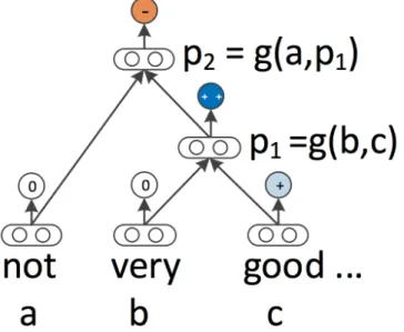
Although semantic vector spaces have been used widely to represent single words, they cannot represent longer phrases appropriately. The problem is that capturing such pat-tern in the sentences requires powerful models and large training resources. To remedy this, the Stanford Sentiment Treebank and the Recursive Neural Tensor Network (RNTN) [62] are used to predict the compositional semantic effects. Figure 3.2 shows one ex-ample of RNTN with clear compositional structure. In Figure 3.2, RNTN can capture the negation and its scope in the sentence and predict 5 sentiment classes (−−, −, 0, +,
++) at each node of a parse tree.
Figure 3.2.An example of RNTN [62].
3.3.1 Stanford Sentiment Treebank
The Stanford Sentiment Treebank is a corpus with labeled parse trees, which allowing us to analyze completely the sentiment in a language [62]. The original dataset of movie reviews, including 10,662 single sentences, was initially collected by Pang and Lee [45]. Moreover, half sentences of this dataset were considered negative and the other half positive. All these sentences were parsed with the Stanford Parser [32], thereby result-ing 215,154 unique phrases from these parse trees [62]. These phrases are labeled with Amazon Mechanical Turk, forming the corpus of Stanford Sentiment Treebank. This new corpus provides the community with the possibility to train compositional models by machine learning techniques [62].
Figure 3.3 illustrates the normalized histogram of sentiment labels at eachn-gram length. The authors noticed that longer phrases often represented stronger sentiment and the majority of the shorter phrases were neutral [62]. Since the extreme values were quite rare, the labels of the Stanford Sentiment Treebank only covered 5 classes: negative, somewhat negative, neutral, somewhat positive and positive [62].
Figure 3.4. Approach of computing compositional vector representations for phrases [62].
3.3.2 Recursive Neural Models
Figure 3.4 displays the approach of computing compositional vector representations for phrases. When an n-gram is given as an input, a binary tree is built up by parsing the input into separate words which are corresponding to each leaf node. The recursive neutral model will then use various functionsgto compute parent vectors in a bottom up fashion. And the parent vectors will work as features for classification.
Ad-dimensional vector is utilized to represent each word. And the word vector is initialized by randomly sampling from a uniform distribution: U(−r, r), where r = 0.0001[62]. The embedding matrix L ∈ ℜd×|V| stacks all the word vectors, and |V|indicates the size of the vocabulary. Moreover, the word vectors can work as features and also parameters to optimize a sof tmaxclassifier [62]. For five-class classification, the posterior probability with labels is computed based on the word vector:
ya=sof tmax(Wsa) (3.1)
whereWs∈ ℜ5×dis the sentiment classification matrix. Similarly, we can get the posterior probability for the vectorsbandcin Figure 3.4 using the same step.
text mining. The Equations 3.2 represent that how RNNs compute the parent vectors: p1=f ⎛ ⎝W ⎡ ⎣ b c ⎤ ⎦ ⎞ ⎠, p2 =f ⎛ ⎝W ⎡ ⎣ a p1 ⎤ ⎦ ⎞ ⎠ (3.2)
wheref =tanhdenotes a standard element-wise nonlinearity,W ∈ ℜd×2d indicates the main parameters, and the bias is omitted for simplicity. The parent vectors must have the same dimensionality and each parent vector pi uses the samesof tmaxfunction of Equation 3.1 to compute its label probability.
Most parameters of Matrix-Vector RNN (RNN) are associated with words. The MV-RNN uses both a vector and a matrix to represent each word or phrase in a parse tree [62]. The matrix of every word is initialized as ad×didentity matrix with a minor number of Gaussian noise. For the parse tree containing vector and matrix nodes, the MV-RNN computes the first parent vector and its matrix:
p1=f ⎛ ⎝W ⎡ ⎣ Cb Bc ⎤ ⎦ ⎞ ⎠, P1 =f ⎛ ⎝WM ⎡ ⎣ B C ⎤ ⎦ ⎞ ⎠ (3.3)
whereWM ∈ ℜd×2dis ad×dmatrix. Similarly, we can compute the second parent node using the previous (vector, matrix) pair (p1,P1).
3.3.3 Recursive Neural Tensor Network
However, both RNN and MV-RNN have their own problems. The problem of RNN is that the input vectors only implicitly interact through the non-linearity function, and the number of parameters in MV-RNN is too large for processing. In order to address these problems, the authors proposed a more powerful single composition model: the Recursive Neural Tensor Network (RNTN). For all nodes in the parse tree, RNTN attempts to use the same and tensor-based composition function, which is also the core idea of RNTN [62].
For each sliceV[i]∈ ℜd×d, the output of a tensor producth∈ ℜdis defined as:
h= ⎡ ⎣ b c ⎤ ⎦ T V[1:d] ⎡ ⎣ b c ⎤ ⎦;hi = ⎡ ⎣ b c ⎤ ⎦ T V[i] ⎡ ⎣ b c ⎤ ⎦ (3.4)
The RNTN uses this definition to computep1: p1=f ⎛ ⎜ ⎝ ⎡ ⎣ b c ⎤ ⎦ T V[1:d] ⎡ ⎣ b c ⎤ ⎦+W ⎡ ⎣ b c ⎤ ⎦ ⎞ ⎟ ⎠ (3.5)
whereW is the same with that defined in the previous models. The same weights can be used to compute the next parent vectorp2in Figure 3.4:
p2 =f ⎛ ⎜ ⎝ ⎡ ⎣ a p1 ⎤ ⎦ T V[1:d] ⎡ ⎣ a p1 ⎤ ⎦+W ⎡ ⎣ a p1 ⎤ ⎦ ⎞ ⎟ ⎠ (3.6)
The following part describes the training step for the RNTN model. As explained above, each node predicts the target vector t via a sof tmax classifier which is trained on its vector representation. It is assumed that the target distribution vector at each node has a 0-1 encoding [62]. If there areC classes, the assumption is that the target vector has lengthC and all other entries are 0 except a 1 at the correct label.
The error function of the RNTN parametersθ= (V, W, Ws, L)for a sentence is:
E(θ) =∑
i
∑
j
tijlogyji +λ||θ||2 (3.7)
xi denotes the vector at nodei. Each node back-propagates its error to the recursively used weightsV,W. Thenδi,s∈ ℜd×1will be thesof tmaxerror vector at nodei:
δi,s=( WsT ( yi−ti)) ⊗f′( xi) (3.8) where⊗is the Hadamard product between the two vectors.f′is the element-wise deriva-tive off =tanh.
For the derivative of each slicek= 1, . . . , d:
∂Ep2 ∂V[k] =δ p2,com k ⎡ ⎣ a p1 ⎤ ⎦ ⎡ ⎣ a p1 ⎤ ⎦ T (3.9) whereδp2,com
k is thek’th element. Next, the error message for the two children ofp2 can be computed: δp2,down=( WTδp2,com+S) ⊗f′ ⎛ ⎝ ⎡ ⎣ a p1 ⎤ ⎦ ⎞ ⎠ (3.10)
where S = d ∑ k=1 δpk2,com ( V[k]+(v[k])T ) ⎡ ⎣ a p1 ⎤ ⎦ (3.11)
The completeδcomes from two parts. One is that the children ofp2each take half of this
vector and the other is their ownsof tmaxerror message [62]. Then we have:
δp1,com =δp1,s+δp2,down[d+ 1 : 2d] (3.12)
wherep1 is the right child ofp2 and hence takes the2nd half of the error ofp2.
For the tri-gram tree in Figure 3.4, the full derivative for sliceV[k]is calculated:
∂E ∂V[k] = Ep2 ∂V[k]+δ p1,com k ⎡ ⎣ b c ⎤ ⎦ ⎡ ⎣ b c ⎤ ⎦ T (3.13)
and similarly forW.
3.4 Data
Using gold standard labeled datasets is a key aspect in comparing sentiment analysis methods. Table 3.2 presents the main characteristics of seven datasets covering a wide range of sources. For example, the number of messages, the number of messages in each sentiment class, and the average number of words per message are summarized in Table 3.2. "#Pos" indicates the positive class, "#Neg" means the negative class, and "#Neu" states the neutral class. Additionally, Table 3.2 also states the methodology ap-plied in the sentiment classification. Labeling with Amazon Mechanical Turk (AMT) was carried out in three out of the seven datasets, while the left datasets use volunteers and other strategies which contain non-expert annotators. Generally, an agreement strategy, such as majority voting, ensures that each sentence has an agreed-upon polarity in each dataset. Table 3.2 also shows the number of evaluators who labeled the datasets. The New York Times (NYT) is an American newspaper which has significant worldwide influence and readership. The NYT provides its readers with different sections on various topics, such as sports, arts, science, home, and travel. Comments_NYT includes 5190 sentence-level snippets from 500 New York Times opinion editorials [20]. This dataset was labeled with AMT, and there are 2204 positive messages, 2742 negative messages and 244 neutral messages.
TED (www.ted.com) is a popular media organization which posts public talks and user-contributed material (favorites, comments) [48]. It is an online repository that includes
talks on many political, scientific, academic, and cultural topics under a Creative Com-mons license. The authors of Comments_TED crawled the TED website in September 2012, and they collected sentences from 74,760 users and 1,203 talks, with 134,533 favorites and 209,566 comments [48]. Comments_TED, including 839 comments, is a subset of original dataset with 839 positive sentences, 318 negative sentences and 409 neutral sentences.
YouTube is a popular American video-sharing website, allowing its users to watch, share, and comment on videos. YouTube provides a wide range of contents, such as movie trailers, music videos, documentary films, and TV shows. Comments_YTB includes 3407 text comments posted to videos on the YouTube website [65]. In Comments_YTB, there are 1665 positive comments, 767 negative comments and 975 neutral comments. Myspace is a social networking website, offering an interactive network of friends, blogs, photos, personal profiles, groups, videos, and music. Myspace was the most common so-cial networking from 2005 to 2009 in the world [65]. In this thesis, Myspace is a corpus of 1041 comments from the social network site MySpace, including 702 positive comments, 132 negative comments and 207 neutral comments [65].
Twitter is a microblogging site in the Web. Furthermore, we usually gather tweets which express sentiment on popular topics from Twitter. Tweets_Semeval is the dataset used in SemEval-2013 task 2, and the authors first used a Twitter-tuned NER system to extract name entities from millions of tweets, which they gathered over a one-year period ranging from January 2012 to January 2013 [39]. Here, Tweets_Semeval is just a subset of the original dataset with 6087 tweets, including 2223 positive tweets, 837 negative tweets and 3027 neutral tweets.
Tweets_RND_I comes from Thewall’s study that attempted to explore the representative patterns of sentiment changes in an event. In addition, the data was used to determine whether sentiment changes could indicate the amount of interest in an event during the early sta
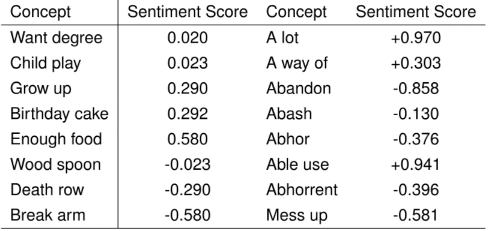
![Figure 3.3. The normalized histogram of sentiment labels at each n-gram length [62].](https://thumb-us.123doks.com/thumbv2/123dok_us/59786.2507075/32.892.178.801.811.1093/figure-normalized-histogram-sentiment-labels-n-gram-length.webp)