Database Management
Subject: DATABSE MANAGEMENT
Credits: 4
SYLLABUS
Introduction to data base management system – Data versus information, record, file; data dictionary, database
administrator, functions and responsibilities; file-oriented system versus database system
Database system architecture – Introduction, schemas, sub schemas and instances; data base architecture, data
independence, mapping, data models, types of database systems
Data base security – Threats and security issues, firewalls and database recovery; techniques of data base
security; distributed data base
Data warehousing and data mining – Emerging data base technologies, internet, database, digital libraries,
multimedia data base, mobile data base, spatial data base
Lab:
Working over Microsoft Access
Suggested Readings:
1.
A Silberschatz, H Korth, S Sudarshan, “Database System and Concepts”; fifth Edition; McGraw-Hill
2.
Rob, Coronel, “Database Systems ”, Seventh Edition, Cengage Learning
DATABASE MANAGEMENT
D A T A B A S E M A N A G E M E N T S Y S T E M
COURSE OVERVIEW
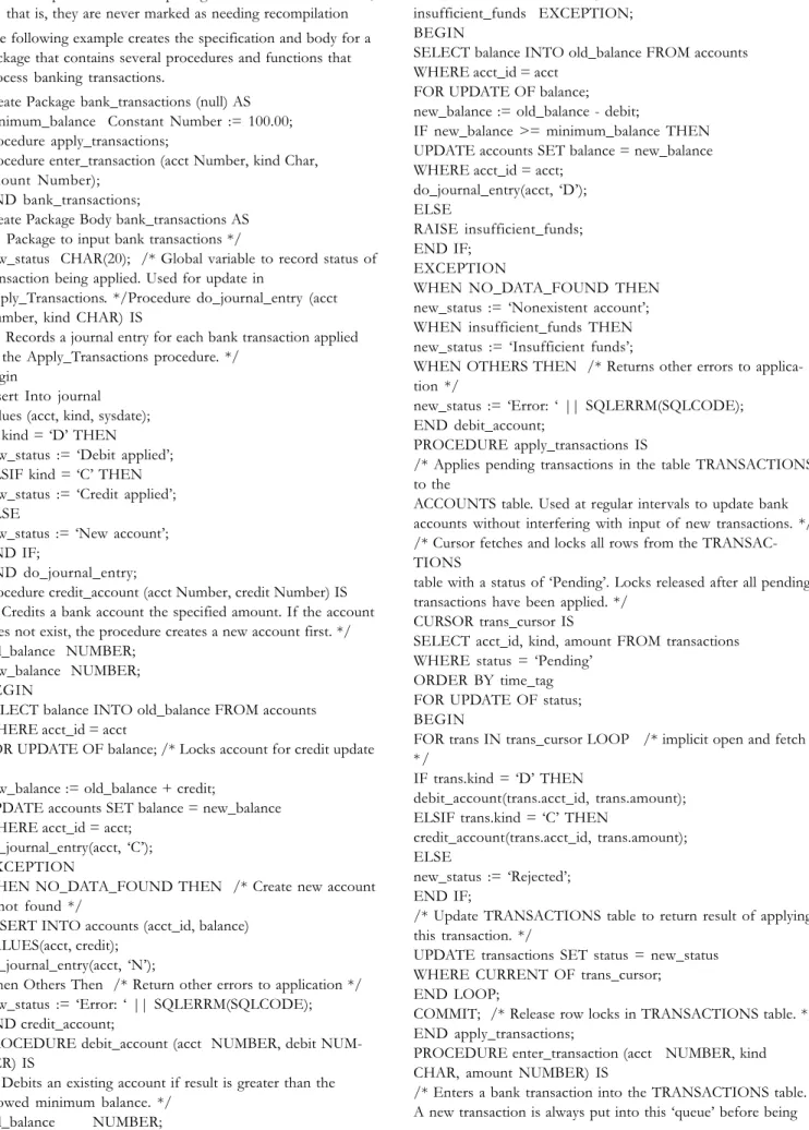
This course provides an immediately useable tools and the techniques in the methods of database management system, requirements analysis, definition, specification and design etc. It provides participants with the details if the tools, techniques and methods to lead or participate in the front-end phases. Database systems are designed to manage large bodies of information.Management of data involves both defining structures for storage of information & providing way for manipulation of data. In addition, the database system must ensure safety of data.
DBMS is collection of programs that enables you to store, modify, and extract important information from a database. There are many different types of DBMS, ranging from small sys-tems that run on personal computers to huge systems that run on mainframes.
Objectives
• To help you to learn DBMS and design technique: what it is and how one goes about doing it.
• The primary goal of DBMS is to provide an environment that is both convenient & efficient for people to use in retrieving & storing information..
• Database systems are designed to store large bodies of information.
By the end of this material, you will be equipped with good knowledge of technical information that will help you develop & understand DBMS
The students on completion of the course shall develop the following skills and competencies:
• Database
• DBMS
• Database System Application • File System
DATABASE MANAGEMENT
Lesson No. Topic Page No.
Lesson 1 Introduction to Database I 1 Lesson 2 Introduction to Database II 5 Lesson 3 Tutorial 8 Lesson 4 Database Concepts I 9 Lesson 5 Database Concepts II 13
Lesson 6 Data Models 17
Lesson 7 Relational Database Management System I 21 Lesson 8 Relational Database Management System II 27
Lesson 9 E-R ModelI 31
Lesson 10 E-R Model II 36
Lesson 11 Structured Query Language(SQL) I 40
Lesson 12 LAB 45 Lesson 13 Lab 46 Lesson 14 SQLII 47 Lesson 15 LAB 55 Lesson 16 LAB 56 Lesson 17 SQLIII 57 Lesson 18 Lab 62 Lesson 19 Lab 63 Lesson 20 SQLIV 64 Lesson 21 Lab 67 Lesson 22 Lab 68
Lesson 23 Integrity and security 69
Lesson 24 LAB 75
Lesson 25 LAB 76
Lesson 26 PL/SQL 77
Lesson 27 Lab 82
Lesson 28 Lab 83
Lesson 29 Database Triggers 84
Lesson 30 LAB 89
C O N T E N T
D A T A B A S E M A N A G E M E N T
RELATIONAL DATA BASE MANAGEMENT SYSTEM
STRUCTURED QUERY LANGUAGES INTRODUCTION TO DBMS
DATABASE MANAGEMENT
Lesson No. Topic Page No.
Lesson 31 LAB 90
Lesson 32 Database Cursors 91
Lessom 33 LAB 100
Lesson 34 LAB 101
Lesson 35 NormalisationI 102
Lesson 36 Normalisation I I 107 Lesson 37 Normalisation III 112
Lesson 38 File Organization Method I 118
Lesson 39 File Organization Method II 123
Lesson 40 Transactions Management 130
Lesson 41 Concurrency Control I 136 Lesson 43 Concurrency Control III 146
C O N T E N T
D A T A B A S E M A N A G E M E N T
NORMALIZATION
FILE ORGANIZATION METHODS
Lesson 42 Concurency Control II 141
DATA BASE OPERATIONAL MAINTENANCE
DATABASE MANAGEMENT
LESSON 1:
INTRODUCTION TO DATABASE I
Lessons Objective
• Database• Database management system • Essentials of data
• Benefits of DBMS
• Database system application • Purpose of database system
1.1 What is Database Management
System(DBMS)
A database can be termed as a repository of data. A collection of actual data which constitutes the information regarding an organisation is stored in a database. For ex. There are 1000 students in a college & we have to store their personal details, marks details etc., these details will be recorded in a database. A collection of programs that enables you to store, modify, and extract information from a database is known as DBMS.The primary goal of a DBMS is to provide a way to store & retrieve database information that is both convenient & efficient.
Database systems are designed to manage large bodies of information.Management of data involves both defining structures for storage of information & providing way for manipulation of data. In addition, the database system must ensure safety of data.
DBMS is collection of programs that enables you to store, modify, and extract important information from a database. There are many different types of DBMS, ranging from small sys-tems that run on personal computers to huge systems that run on mainframes.
Good data management is an essential prerequisite to corporate success. Data Information Information Knowledge Knowledge Judgment Judgment Decision Decision Success
provided that data is: • complete • accurate • timely • easily available
1.2 Database System Applications
There are many different types of DBMSs, ranging from small systems that run on personal computers to huge systems that run on mainframes. Database are applied in wide no. of applications. Following are some of the examples
:-• Banking: For customer information, accounts, loans & other banking transactions
• Airlines: For reservation & schedule information • Universities: For student information, course
registration,grades etc.
• Credit card transaction: For purchase of credit cards & generation of monthly statements.
• Tlecommunication: For keeping records of calls made , generating monthly billetc.
• Finance: For storing information about holdings, sales & purchase of financial statements
• Sales: For customer,product & purchase information • Manufacturing: For management of supply chain. • Human Resource: For recording information about
employees,salaries,tax,benefits etc.
We can say that when ever we need to have a computerised system, we need a database system
1.3 Purpose of Database system
A file system is one in which we keep the information in operating system files. Before the evolution of DBMS, organisations used to store information in file systems. A typical file processing system is supported by a conventional operating system. The system stores permanent records in various files & it need application program to extract records , or to add or delete records .We will compare both systems with the help of an example. There is a saving bank enterprise that keeps information about all customers & saving accounts. Following manipulations has to be done with the system
• A program to debit or credit an account • A program to add a new account. • A program to find balance of an account. • A program to generate monthly statements.
As the need arises new applications can be added at a particular point of time as checking accounts can be added in a saving account. Using file system for storing data has got following
disadvantages:-1. Data Redundancy and Inconsistency
Different programmers work on a single project , so various files are created by different programmers at some interval of time. So various files are created in different formats & different programs are written in different programming language. Actual data
DATABASE MANAGEMENT
Same information is repeated.For ex name & address may appear in saving account file as well as in checking account. This redundancy sesults in higher storage space & access cost.It also leads to data inconsistency which means that if we change some record in one place the change will not be reflected in all the places. For ex. a changed customer address may be reflected in saving record but not any where else.
2. Difficulty in Accesing data
Accessing data from a list is also a difficulty in file
system.Suppose we want to see the records of all customers who has a balance less than $10,000, we can either check the list & find the names manually or write an application program .If we write an application program & at some later time, we need to see the records of customer who have a balance of less than $20,000, then again a new program has to be written.
It means that file processing system do not allow data to be accessed in a convenient manner.
3. Data Isolation
As the data is stored in various files, & various files may be stored in different format, writing application program to retrieve the data is difficult.
4. Integrity Problems
Sometimes, we need that data stored should satisfy certain constraints as in a bank a minimum deposit should be of $100. Developers enforce these constraints by writing appropriate programs but if later on some new constraint has to be added then it is difficult to change the programs to enforce them.
5. Atomicity Problems
Any mechanical or electrical devive is subject to failure, and so is the computer system. In this case we have to ensure that data should be restored to a consistent state.For example an amount of $50 has to be transferred from Account A to Account B. Let the amount has been debited from account A but have not been credited to Account B and in the mean time, some failure occurred. So, it will lead to an inconsistent state.
So,we have to adopt a mechanism which ensures that either full transaction hould b executed or no transaction should be excuted i.e. the fund transfer should be atomic.
6. Concurrent access Problems
Many systems allows multiple users to update the data simultaneously. It can also lead the data in an inconsistent state.Suppose a bank account contains a balance of $ 500 & two customers want to withdraw $100 & $50 simultaneously. Both the transaction reads the old balance & withdraw from that old balance which will result in $450 & &400 which is incorrect.
7.Security Problems
All the user of database should not be able to access all the data. For example a payroll
Personnel needs to access only that part of data which has information about various employees & are not needed to access information about customer accounts.
Points to Ponder
• A DBMS contains collection of inter-related data & collection of programs to access the data.
• The primary goal of DBMS is to provide an environment that is both convenient & efficient for people to use in retrieving & storing information.
• DBMS systems are ubiquitous today & most people interact either directly or indirectly with database many times every day.
• Database systems are designed to store large bodies of information.
• A major purpose of a DBMS is to provide users with an abstract view of data i.e. the system hides how the data is stored & maintained.
Review Terms
• Database• DBMS
• Database System Application • File System • Data Ionsistency • Consistency constraints • Atomicity • Redundancy • Data isolation • Data Security
Students Activity
1. What is database?Explain with example?
2. What is DBMS?Explain with example?
3. List four significant difference between file system & DBMS?
DATABASE MANAGEMENT 4. What are the advantages of DBMS?
5. Explain various applications of database?
6. Explain data inconsistency with example?
7. Explain data security? Why it is needed?Explain with example?
8. Explain isolation & atomicity property of database?
9. Explain why redundancy should be avoided in database?
DATABASE MANAGEMENT
DATABASE MANAGEMENT
Lesson Objective
• Data abstraction • View of data • Levels of data • Physical level • Logical level • View level • Database language • DDL,DMLView of Data
A database contains a no. of files & certain programs to access & modify these files.But the actual data is not shown to the user, the system hides actual details of how data is stored & main-tained.
Data Abstraction
Data abstraction is the process of distilling data down to its essentials. The data when needed should be retrieved efficiently. As all the details are not of use for all the users, so we hide the actual(complex) details from users. Various level of abstraction to data is provided which are listed
below:-• Physical level
It is the lowest level of abstraction & specifies how the data is actually stored. It describes the complex data structure in details.
• Logical level
It is the next level of abstraction & describes what data are stored in database & what relationship exists between varius data. It is less complex than physical level & specifies simple structures. Though the complexity of physical level is required at logical level, but users of logical level need not know these complexities.
LESSON 2:
INTRODUCTION TO DATABASE II
• View level
This level contains the actual data which is shown to the users. This is the highest level of abstraction & the user of this level need not know the actual details(complexity) of data storage.
Database Language
As a language is required to understand any thing, similarly to create or manipulate a database we need to learn a
language.Database language is divided into mainly 2 parts :-1. DDL(Data definition language)
2. DML(Data Manipulation language)
Data Definition Language (DDL)
Used to specify a database scheme as a set of definitions expressed in a DDL1. DDL statements are compiled, resulting in a set of tables stored in a special file called a data dictionary or data directory.
2. The data directory contains metadata (data about data) 3. The storage structure and access methods used by the
DATABASE MANAGEMENT
special type of DDL called a data storage and definition language
4. basic idea: hide implementation details of the database schemes from the users
Data Manipulation Language (DML)
1. Data Manipulation is:• retrieval of information from the database • insertion of new information into the database • deletion of information in the database • modification of information in the database 2. A DML is a language which enables users to access and
manipulate data. The goal is to provide efficient human interaction with the system.
3. There are two types of DML:
• procedural: the user specifies what data is needed and how to get it
• nonprocedural: the user only specifies what data is needed
• Easier for user
• May not generate code as efficient as that produced by procedural languages
4. A query language is a portion of a DML involving information retrieval only. The terms DML and query language are often used synonymously.
Points to Ponder
• DBMS systems are ubiquitous today & most people interact either directly or indirectly with database many times every day.
• Database systems are designed to store large bodies of information.
• A major purpose of a DBMS is to provide users with an abstract view of data i.e. the system hides how the data is stored & maintained.
• Structure of a database is defined through DDL. & manipulated through DML.
• DDL statements are compiled, resulting in a set of tables stored in a special file called a data dictionary or data directory.
• A query language is a portion of a DML involving information retrieval only. The terms DML and query language are often used synonymously.
Review Terms
• Data Security • Data Views • Data Abstraction • Physical level • Logical level • View level • Database language • Ddl • Dml • Query languageStudents Activity
1. Define data abstraction?2. How many views of data abstraction are there? Explain in details?
3. Explain database language? Differentiate between DDL & DML?
DATABASE MANAGEMENT
DATABASE MANAGEMENT
LESSON 3:
TUTORIAL
DATABASE MANAGEMENT
Lesson objective
• Data dictionary • Meta data • Database schema • Database Instance • Data independenceData Dictionary
English language dictionaries define data in terms such as “…known facts or things used as a basis for inference or reckoning, typically (in modern usage) operated upon or manipulated by computers, or Factual information used as a basis for discussion, reasoning, or calculation
Data dictionary may cover the whole organisation, a part of the organisation or a database. In its simplest form, the data dictionary is only a collection of data element definitions. More advanced data dictionary contains database schema with reference keys, still more advanced data dictionary contains entity-relationship model of the data elements or objects.
Parts of Data Dictionary
1. Data Element Definitions
Data element definitions may be independent of table defini-tions or a part of each table definition
• Data element number
Data element number is used in the technical documents. • Data element name (caption)
Commonly agreed, unique data element name from the application domain. This is the real life name of this data element.
• Short description
Description of the element in the application domain. • Security classification of the data element
Organisation-specific security classification level or possible restrictions on use. This may contain technical links to security systems.
• Related data elements
List of closely related data element names when the relation is important.
• Field name(s)
Field names are the names used for this element in computer programs and database schemas. These are the technical names, often limited by the programming languages and systems.
• Code format
Data type (characters, numeric, etc.), size and, if needed, special representation. Common programming language notation, input masks, etc. can be used.
• Null value allowed
Null or non-existing data value may be or may not be allowed for an element. Element with possible null values needs special considerations in reports and may cause problems, if used as a key.
• Default value
Data element may have a default value. Default value may be a variable, like current date and time of the day (DoD). • Element coding (allowed values) and intra-element
validation details or reference to other documents
Explanation of coding (code tables, etc.) and validation rules when validating this element alone in the application domain.
• Inter-element validation details or reference to other documents
Validation rules between this element and other elements in the data dictionary.
• Database table references
Reference to tables the element is used and the role of the element in each table. Special indication when the data element is the key for the table or a part of the key. • Definitions and references needed to understand the
meaning of the element
Short application domain definitions and references to other documents needed to understand the meaning and use of the data element.
• Source of the data in the element
Short description in application domain terms, where the data is coming. Rules used in calculations producing the element values are usually written here.
• Validity dates for the data element definition
Validity dates, start and possible end dates, when the element is or was used. There may be several time periods the element has been used.
• History references
Date when the element was defined in present form, references to superseded elements, etc.
• External references
References to books, other documents, laws, etc. • Version of the data element document
Version number or other indicator. This may include formal version control or configuration management references, but such references may be hidden, depending on the system used.
• Date of the data element document
Writting date of this version of the data element document.
LESSON 4:
DATABASE MANAGEMENT
• Quality control references
Organisation-specific quality control endorsements, dates, etc.
• Data element notes
Short notes not included in above parts.
Table Definitions
Table definition is usually available with SQL command help table
Tablename • Table name
• Table owner or database name
• List of data element (column) names and details • Key order for all the elements, which are possible keys • Possible information on indexes
• Possible information on table organisation
Technical table organisation, like hash, heap, B+ tree, AVL -tree, ISAM, etc. may be in the table definition.
• Duplicate rows allowed or not allowed
• Possible detailed data element list with complete data element definitions
• Possible data on the current contents of the table The size of the table and similar site specific information may be kept with the table definition.
• Security classification of the table
Security classification of the table is usually same or higher than its elements. However, there may be views accessing parts of the table with lower security.
Database schema
It is the overall structure is called a database schema. Database schema is usually graphical presentation of the whole database. Tables are connected with external keys and key colums. When accessing data from several tables, database schema will be needed in order to find joining data elements and in complex cases to find proper intermediate tables. Some database products use the schema to join the tables automatically. Database system has several schemas according to the level of abstraction.The physical schema describes the database design at physical level. The logical schema describes the database design at logical level.A database can also have sub-schemas(view level) that describes different views of database.
Database Instance
1. Databases change over time.
2. The information in a database at a particular point in time is called an instance of the database
3. Analogy with programming languages: • Data type definition - scheme • Value of a variable - instance
Meta-Data
Meta-data is definitional data that provides information about or documentation of other data managed within an application or environment.
For example, meta-data would document data about data elements or attributes, (name, size, data type, etc) and data about records or data structures (length, fields, columns, etc) and data about data (where it is located, how it is associated, ownership, etc.). Meta-data may include descriptive information about the context, quality and condition, or characteristics of the data.
Data Independence
1. The ability to modify a scheme definition in one level without affecting a scheme definition in a higher level is called data independence.
2. There are two kinds:
• Physical data independence
• The ability to modify the physical scheme without causing application programs to be rewritten • Modifications at this level are usually to improve
performance
• Logical data independence
• The ability to modify the conceptual scheme without causing application programs to be rewritten
• Usually done when logical structure of database is altered
3. Logical data independence is harder to achieve as the application programs are usually heavily dependent on the logical structure of the data. An analogy is made to abstract data types in programming languages.
Points to Ponder
• Data dictionary is a collection of data elements & its definition.
• Database Schema is the overall structure of a database. • Database instance is the structure of a database at a
particular time.
• Meta-data is the data about data.
• The ability to modify a scheme definition in one level without affecting a scheme definition in a higher level is called data independence.
Review Terms
• Database Instance • Schema Database Schema Physical schema Logical schema • Physical data independence • Database Language DDL DML Query Language • Data dictionary • MetadataDATABASE MANAGEMENT
Student Activity
1. What is difference between database Schema & database instance?
2. What do you understand by the structure of a database?
3. Define physical schema and logical schema?
4. Define data independence?Explain types of data independence?
5. Define data dictionary, meta-data?
DATABASE MANAGEMENT
DATABASE MANAGEMENT
Lesson Objective
• Database manager • Database user• Database administrator • Role of Database administrator • Role of Database user
• Database architecture
Database Manager
The database manager is a program module which provides the interface between the low-level data stored in the database and the application programs and queries submitted to the system. 1. Databases typically require lots of storage space (gigabytes). This must be stored on disks. Data is moved between disk and main memory (MM) as needed.
2. The goal of the database system is to simplify and facilitate access to data. Performance is important. Views provide simplification.
3. So the database manager module is responsible for • Interaction with the file manager: Storing raw data
on disk using the file system usually provided by a conventional operating system. The database manager must translate DML statements into low-level file system commands (for storing, retrieving and updating data in the database).
• Integrity enforcement: Checking that updates in the database do not violate consistency constraints (e.g. no bank account balance below $25)
• Security enforcement: Ensuring that users only have access to information they are permitted to see • Backup and recovery: Detecting failures due to
power failure, disk crash, software errors, etc., and restoring the database to its state before the failure • Concurrency control: Preserving data consistency
when there are concurrent users.
4. Some small database systems may miss some of these features, resulting in simpler database managers. (For example, no concurrency is required on a PC running MS-DOS.) These features are necessary on larger systems
Database Administrator
The database administrator is a person having central control over data and programs accessing that data. Duties of the database administrator include:
• Scheme definition: the creation of the original database scheme. This involves writing a set of definitions in a DDL (data storage and definition language), compiled by the DDL compiler into a set of tables stored in the data dictionary.
• Storage structure and access method definition: writing a set of definitions translated by the data storage and definition language compiler
• Scheme and physical organization modification: writing a set of definitions used by the DDL compiler to generate modifications to appropriate internal system tables (e.g. data dictionary). This is done rarely, but sometimes the database scheme or physical organization must be modified. • Granting of authorization for data access: granting
different types of authorization for data access to various users
• Integrity constraint specification: generating integrity constraints. These are consulted by the database manager module whenever updates occur.
Database Users
The database users fall into several categories:
Application programmers are computer professionals interact-ing with the system through DML calls embedded in a program written in a host language (e.g. C, PL/1, Pascal).
• These programs are called application programs. • The DML precompiler converts DML calls (prefaced by a
special character like $, #, etc.) to normal procedure calls in a host language.
• The host language compiler then generates the object code. • Some special types of programming languages combine
Pascal-like control structures with control structures for the manipulation of a database.
• These are sometimes called fourth-generation languages. • They often include features to help generate forms and
display data.
• Sophisticated users interact with the system without writing programs.
• They form requests by writing queries in a database query language.
• These are submitted to a query processor that breaks a DML statement down into instructions for the database manager module.
• Specialized users are sophisticated users writing special database application programs. These may be CADD systems, knowledge-based and expert systems, complex data systems (audio/video), etc.
• Naive users are unsophisticated users who interact with the system by using permanent application programs (e.g. automated teller machine).
1. Database systems are partitioned into modules for different functions. Some functions (e.g. file systems) may be provided by the operating system.
LESSON 5:
DATABASE MANAGEMENT
2. Components include:
• File manager manages allocation of disk space and data structures used to represent information on disk. • Database manager: The interface between low-level
data and application programs and queries. • Query processor translates statements in a query
language into low-level instructions the database manager understands. (May also attempt to find an equivalent but more efficient form.)
• DML precompiler converts DML statements embedded in an application program to normal procedure calls in a host language. The precompiler interacts with the query processor.
• DDL compiler converts DDL statements to a set of tables containing metadata stored in a data dictionary. In addition, several data structures are required for physical system implementation:
• Data files: store the database itself.
• Data dictionary: stores information about the structure of the database. It is used heavily. Great emphasis should be placed on developing a good design and efficient
implementation of the dictionary.
• Indices: provide fast access to data items holding particular values.
Database System Architecture
Database systems are partitioned into modules for different functions. Some functions (e.g. file systems) may be provided by the operating system.
Components Include
• File manager manages allocation of disk space and data structures used to represent information on disk. • Database manager: The interface between low-level data
and application programs and queries.
• Query processor translates statements in a query language into low-level instructions the database manager
understands. (May also attempt to find an equivalent but more efficient form.)
• DML precompiler converts DML statements embedded in an application program to normal procedure calls in a host language. The precompiler interacts with the query processor.
• DDL compiler converts DDL statements to a set of tables containing metadata stored in a data dictionary.
In addition, several data structures are required for physical system implementation:
• Data files: store the database itself.
• Data dictionary: stores information about the structure of the database. It is used heavily. Great emphasis should be placed on developing a good design and efficient
implementation of the dictionary.
• Indices: provide fast access to data items holding particular values. DML PreCompiler Query processor DDL compiler Application Program object code Database Manager File Manager Data files Data dictionary Data storage Naïve
Users Application Programs
Sophisticated Users
Database Administrator
Application
Interfaces Application programs Query Database Schema
Points to Ponder
• Database manager is a program module which provides the interface between the low-level data stored in the database and the application programs
• Database administrator is a person having central control over data
• Database user is a person who access the database at various level.
• Data files: store the database itself.
• Data dictionary: stores information about the structure of the database.
• DML precompiler converts DML statements embedded in an application program to normal procedure calls in a host language.
• File manager manages allocation of disk space and data structures used to represent information on disk.
Review Terms
• Database Instance • Schema Database Schema Physical schema Logical schema • Physical data independenceDATABASE MANAGEMENT • Database Language DDL DML Query Language • Data dictionary • Metadata • Database Administrator • Database User
Student Activity
1. What are the various kinds of database users?
2. What do you understand by the structure of a database?
3. Define physical schema and logical schema?
DATABASE MANAGEMENT
DATABASE MANAGEMENT
LESSON 6:
DATA MODELS
Lesson objective
• Understsnding data models • Different types of data models • Hierchachical data model • network data model • Relational modelData models are a collection of conceptual tools for describing data, data relationships, data semantics and data constraints. A data model is a “description” of both a container for data and a methodology for storing and retrieving data from that container. Actually, there isn’t really a data model “thing”. Data models are abstractions, oftentimes mathematical algorithms and concepts. You cannot really touch a data model. But nevertheless, they are very useful. The analysis and design of data models has been the cornerstone of the evolution of databases. As models have advanced so has database efficiency. There are various kinds of data models i.e. in a database records can be arranged in various ways.The various ways in which data can be represented
are:-1. Hierarchial data model 2. Network data model 3. Relational Model 4. E-R-Model
The Hierarchical Model
Organization of the records is as a collection of trees. As its name implies, the Hierarchical Database Model defines hierarchi-cally-arranged data.
Perhaps the most intuitive way to visualize this type of relationship is by visualizing an upside down tree of data. In this tree, a single table acts as the “root” of the database from which other tables “branch” out.
You will be instantly familiar with this relationship because that is how all windows-based directory management systems (like Windows Explorer) work these days.
Relationships in such a system are thought of in terms of children and parents such that a child may only have one parent but a parent can have multiple children. Parents and children are tied together by links called “pointers” (perhaps physical addresses inside the file system). A parent will have a list of pointers to each of their children.
If we want to create a structure where in a course various students are there & these students are given certain marks in assignment.
However, as you can imagine, the hierarchical database model has some serious problems. For one, you cannot add a record to a child table until it has already been incorporated into the parent table. This might be troublesome if, for example, you wanted to add a student who had not yet signed up for any courses.
Worse, yet, the hierarchical database model still creates repetition of data within the database. You might imagine that in the database system shown above, there may be a higher level that includes multiple course. In this case, there could be redundancy because students would be enrolled in several courses and thus each “course tree” would have redundant student information. Redundancy would occur because hierarchical databases handle one-to-many relationships well but do not handle many-to-many relationships well. This is because a child may only have one parent. However, in many cases you will want to have the child be related to more than one parent. For instance, the relationship between student and class is a “many-to-many”. Not only can a student take many subjects but a subject may also be taken by many students. How would you model this relationship simply and efficiently using a hierarchical database? The answer is that you wouldn’t.
Though this problem can be solved with multiple databases creating logical links between children, the fix is very kludgy and awkward.
Faced with these serious problems, the computer brains of the world got together and came up with the network model.
Network Databases
In many ways, the Network Database model was designed to solve some of the more serious problems with the Hierarchical Database Model. Specifically, the Network model solves the problem of data redundancy by representing relationships in terms of sets rather than hierarchy. The model had its origins in
DATABASE MANAGEMENT
the Conference on Data Systems Languages (CODASYL) which had created the Data Base Task Group to explore and design a method to replace the hierarchical model.
The network model is very similar to the hierarchical model actually. In fact, the hierarchical model is a subset of the network model. However, instead of using a single-parent tree hierarchy, the network model uses set theory to provide a tree-like hierarchy with the exception that child tables were allowed to have more than one parent. This allowed the network model to support many-to-many relationships.
Visually, a Network Database looks like a hierarchical Database in that you can see it as a type of tree. However, in the case of a Network Database, the look is more like several trees which share branches. Thus, children can have multiple parents and parents can have multiple children.
Nevertheless, though it was a dramatic improvement, the network model was far from perfect. Most profoundly, the model was difficult to implement and maintain. Most imple-mentations of the network model were used by computer programmers rather than real users. What was needed was a simple model which could be used by real end users to solve real problems.
Relational Model
The relational model was formally introduced by Dr. E. F. Codd in 1970 and has evolved since then, through a series of writings. The model provides a simple, yet rigorously defined, concept of how users perceive data. Network model solves the problem of data redundancy by representing relationships in terms of sets. A relational database is a collection of two-dimensional tables. The organization of data into relational tables is known as the logical view of the database. That is, the form in which a relational database presents data to the user and the programmer. The way the database software physically stores the data on a computer disk system is called the internal view. The internal view differs from product to product and does not concern us here.
A relational database allows the definition of data structures, storage and retrieval operations and integrity constraints. In such a database the data and relations between them are organised in tables. A table is a collection of records and each record in a table contains the same fields.
Properties of Relational Tables
• Values Are Atomic• Each Row is Unique
• Column Values Are of the Same Kind
• The Sequence of Columns is Insignificant • The Sequence of Rows is Insignificant • Each Column Has a Unique Name
Certain fields may be designated as keys, which means that searches for specific values of that field will use indexing to speed them up. Where fields in two different tables take values from the same set, a join operation can be performed to select related records in the two tables by matching values in those fields. Often, but not always, the fields will have the same name in both tables. For example, an “orders” table might contain (customer-ID, product-code) pairs and a “products” table might contain (product-code, price) pairs so to calculate a given customer’s bill you would sum the prices of all products ordered by that customer by joining on the product-code fields of the two tables. This can be extended to joining multiple tables on multiple fields. Because these relationships are only specified at retreival time, relational databases are classed as dynamic database management system. The RELATIONAL database model is based on the Relational Algebra.
A basic understanding of the relational model is necessary to effectively use relational database software such as Oracle, Microsoft SQL Server, or even personal database systems such as Access or Fox, which are based on the relational model.
Points to Ponder
• Data models are a collection of conceptual tools for describing data, data relationships, data semantics and data constraints.
• Types of data models are:-1. Hierarchial data model 2. Network data model 3. Relational Model 4. E-R-Model
• The Hierarchical Database Model defines hierarchically-arranged data.
• Network model solves the problem of data redundancy by representing relationships in terms of sets.
• Network model solves the problem of data redundancy by representing relationships in terms of sets.
Review Terms
• Data models • Hierchical data model • Network data model • Relational data modelDATABASE MANAGEMENT
Students Activity
1. Define data models?
2. Define hierarchichal data model?
3. Define relational data model?
DATABASE MANAGEMENT
DATABASE MANAGEMENT
LESSON 7:
RELATIONAL DATABASE MANAGEMENT SYSTEM I
Lesson Objective
• Understanding RDBMS • Understanding data structures • Understanding data manipulation• Understanding various relational algebra operation • Understanding data integrity
The relational model was proposed by E. F. Codd in 1970. It deals with database management from an abstract point of view. The model provides specifications of an abstract database management system.To use the database management systems based on the relational model however, users do not need to master the theoretical foundations. Codd defined the model as consisting of the following three components:
1. Data Structure - a collection of data structure types for building the database.
2. Data Manipulation - a collection of operators that may be used to retrieve, derive or modify data stored in the data structures.
3. Data Integrity - a collection of rules that implicitly or explicitly define a consistent database state or changes of states
Data Structure
Often the information that an organisation wishes to store in a computer and process is complex and unstructured. For example, we may know that a department in a university has 200 students, most are full-time with an average age of 22 years, and most are females. Since natural language is not a good language for machine processing, the information must be structured for efficient processing. In the relational model the information is structures in a very simple way
We consider the following database to illustrate the basic concepts of the relational data model.
The above database could be mapped into the following relational schema which consists of three relation schemes. Each relation scheme presents the structure of a relation by specifying its name and the names of its attributes enclosed in parenthe-sis. Often the primary key of a relation is marked by
underlining.
student(student_id, student_name, address) enrolment(student_id, subject_id)
subject(subject_id, subject_name, department)
An example of a database based on the above relational model is:
The relation student
The relation enrolment
We list a number of properties of relations: 1. Each relation contains only one record type. 2. Each relation has a fixed numer of columns that are
explicitly named. Each attribute name within a relation is unique.
3. No two rows in a relation are the same.
4. Each item or element in the relation is atomic, that is, in each row, every attribute has only one value that cannot be decomposed and therefore no repeating groups are allowed. 5. Rows have no ordering associated with them.
6. Columns have no ordering associated with them (although most commercially available systems do).
The above properties are simple and based on practical consider-ations. The first property ensures that only one type of
information is stored in each relation. The second property involves naming each column uniquely. This has several benefits. The names can be chosen to convey what each column is and the names enable one to distinguish between the column and its domain. Furthermore, the names are much easier to remember than the position of the position of each column if the number of columns is large.
The third property of not having duplicate rows appears obvious but is not always accepted by all users and designers of DBMS. The property is essential since no sensible context free
student_id student_name address
8656789 8700074 8900020 8801234 8654321 8712374 8612345 Peta Williams John Smith Arun Kumar Peter Chew Reena Rani Kathy Garcia Chris Watanabe 9, Davis Hall 9, Davis Hall 90, Second Hall 88, Long Hall 88, Long Hall 88, Long Hall 11, Main Street
student_id subject_id
8700074
8900020
8900020
8700074
8801234
8801234
CP302
CP302
CP304
MA111
CP302
CH001
subject_id subject_name department
CP302 CP304 CH001 PH101 MA111 Database Management Software Engineering Introduction to Chemistry Physics Pure Mathematics Comp. Science Comp. Science Chemistry Physics Mathematics
DATABASE MANAGEMENT
meaning can be assigned to a number of rows that are exactly the same.
The next property requires that each element in each relation be atomic that cannot be decomposed into smaller pieces. In the relation model, the only composite or compound type (data that can be decomposed into smaller pieces) is a relation. This simplicity of structure leads to relatively simple query and manipulative languages.
The relation is a set of tuples and is closely related to the concept of relation in mathematics. Each row in a relation may be viewed as an assertion. For exaple, the relation student asserts that a student by the name of Reena Rani has student_id 8654321 and lives at 88, Long Hall. Similarly the relation subject asserts that one of the subjects offered by the Department of Computer Science is CP302 Database Manage-ment.
In the relational model, a relation is the only compound data structure since relation do not allow repeating groups or pointers.
We now define the relational terminology:
Relation - essentially a table
Tuple - a row in the relation
Attribute - a column in the relation
Degree of a relation - number of attributes in the relation
Cardinality of a relation - number of tuples in the relation
Domain - a set of values that an attribute is permitted to take. Same domain may be used by a number of different attributes.
Primary key - as discussed in the last chapter, each relation must have an attribute (or a set of attributes) that uniquely identifies each tuple.
Each such attribute (or a set of attributes) is called a candidate key of the relation if it satisfies the following properties: • (a) the attribute or the set of attributes uniquely identifies
each tuple in the relation (called uniqueness), and
• (b) if the key is a set of attributes then no subset of these attributes has property (a) (called minimality).
There may be several distinct set of attributes that may serve as candidate keys. One of the candidate keys is arbitrarily chosen as the primary key of the relation.
The three relations above student, enrolment and subject have degree 3, 2 and 3 respectively and cardinality 4, 6 and 5 respec-tively. The primary key of the the relation student is student_id, of relation enrolment is (student_id, subject_id), and finally the primary key of relation subject is subject_id. The relation student probably has another candidate key. If we can assume the names to be unique than the student_name is a candidate key. If the names are not unique but the names and address together are unique, then the two attributes (student_id, address) is a candidate key. Note that both student_id and (student_id, address) cannot be candidate keys, only one can. Similarly, for the relation subject, subject_name would be a candidate key if the subject names are unique.
The relational model is the most popular data model for commercial data processing applications.It is very much simple due to which the programmer’s work is reduced.
Data Manipulation
The manipulative part of relational model makes set processing (or relational processing) facilities available to the user. Since relational operators are able to manipulate relations, the user does not need to use loops in the application programs. Avoiding loops can result in significant increase in the produc-tivity of application programmers.
The primary purpose of a database in an enterprise is to be able to provide information to the various users in the enterprise. The process of querying a relational database is in essence a way of manipulating the relations that are the database. For example, one may wish to know
1. names of all students enrolled in CP302, or 2. names of all subjects taken by John Smith.
The Relational Algebra
The relational algebra is a procedural query language. It consists of a set of operations that take one or two relations as input and produce a new relation as their result. The fundamental operations in the relational algebra are select, project, union, set difference, Cartesian product, and rename. In addition to the fundamental operations, there are several other operations-namely, set intersection, natural join, division, and assignment. We will define these operations in terms of the fundamental operations.
Fundamental Operations
The select, project, and rename operations are called unary operations, because they operate on one relation. The other three operations operate on pairs of relations and are, therefore, called binary operations.
Various operations are shown as follows:
The Select Operation
The select operation selects tuples that satisfy a given condition.. The argument relation is in parentheses after the σ. Thus, to select those tuples of the loan relation where the branch is “Perryridge,” we write
σ branch-name = “Perryridge” (loan)
If the loan relation is as shown , then the relation that results from the preceding query will be a different relation.
We can find all tuples in which the amount lent is more than $1200 writing σ amount>1200 (loan) Operation Symbol Projection Selection Renaming Union Intersection Assignment Operation Symbol Cartesian product Join
Left outer join
Right outer join
Full outer join
DATABASE MANAGEMENT In general, we allow comparisons using =, ≠, <, ≤, >, ≥ in the
selection predicate. Furthermore, we can combine several predicates into a larger predicate by using the connectives and (Λ), or (V), and not (¬). Thus, to find those tuples pertaining to loans of more than $1200 made by the Perryridge branch, we write
σ branch-name = “Perryridge” L amount>1200 (loan)
The selection predicate may include comparisons between two attributes. To Illustrate, consider the relation loan-officer that consists of three attributes: customer-name, banker-name, and loan-number, which specifies that a particular banker is the loan officer for a loan that belongs to some customer. To find all customers who have the same name as their loan officer, we can write
σ customer-name = banker-name (loan-officer)
Projection
Projection is the operation of selecting certain attributes from a relation R to form a new relation S. For example, one may only be interested in the list of names from a relation that has a number of other attributes. Projection operator may then be used. Like selection, projection is an unary operator.
II loan-number, amount (loan)
Composition of Relational Operations
The fact that the result of a relational operation is itself a relation is important. Consider the more complicated query “Find those customers who live in Harrison.” We write:II customer-name (σ customer-city = “Harrison” (customer)) Notice that, instead of giving the name of a relation as the argument of the projection operation, we give an expression that evaluates to a relation.
In general, since the result of a relational-algebra operation is of the same type (relation) as its inputs, relational-algebra opera-tions can be composed together into a
Loan number and the amount of the loan.
Relational-algebra expression. Composing relational-algebra operations into relational-algebra expressions in just like composing arithmetic operations (such as +, -, *, and %) into arithmetic expressions.
Cartesian Product
The cartesian product of two tables combines each row in one table with each row in the other table.
Perryridge 1500 loan-number amount L-11 L-14 L-15 L-16 L-17 L-23 L-93 900 1500 1500 1300 1000 2000 500
Example: The table E (for Employee)
Example: The table D (for Department)
• Seldom useful in practice. • Can give a huge result.
The Union Operation
Consider a query to find the names of all bank customers who have either an account or a loan or both. Note that the customer relation does not contain the information, since a customer does not need to have either an account or a loan at the bank. To answer this query, we need the information in the depositor relation and in the borrower relation . We know how to find the names of all customers with a loan in the bank:
II customer-name (borrower)
We also know how to find the names of all customers with an account in the bank:
II customer-name (depositor)
To answer the query, we need the union of these two sets; that is, we need all customer names that appear in either or both of the two relations. We find these data by the binary operation union, denoted, as in set theory, by U. So the expression needed is
II customer-name (borrower) U II customer-name (depositor) There are 10 tuples in the result, even though there are seven distinct borrowers and six depositors. This apparent discrepancy occurs because Smith, Jones, and Hayes are borrowers as well as depositors. Since relations are sets, duplicate values are elimi-nated.
enr ename dept
1 Bill A 2 Sarah C 3 John A customer-name Adams Curry Hayes Jackson Jones Smith Williams Lindsay Johnson Turner dnr dname A Marketing B Sales C Legal
Result Relational algebra
enr ename dept dnr dname E X D 1 Bill A A Marketing 1 Bill A B Sales 1 Bill A C Legal 2 Sarah C A Marketing 2 Sarah C B Sales 2 Sarah C C Legal 3 John A A Marketing 3 John A B Sales 3 John A C Legal
DATABASE MANAGEMENT
Names of all customers who have either a loan or an account. For a union operation r U s to be valid, we require that two conditions hold:
1. The relations r and s must have the same number of attributes.
2. The domains of the ith attribute of r and the ith attribute of s must be the same, for all i.
Note that r and s can be, in general, temporary relations that are the result of relational-algebra expressions.
The Set-Intersection Operation
The first additional-relational algebra operation that we shall define is set intersection ( )I. Suppose that we wish to find all customers who have both a loan and an account. Using set intersection, we can write
IIcustomer-name (borrower) IIcustomer-name (deposi-tor)
Note that we can rewrite any relational algebra expression that uses set intersection by replacing the intersection operation with a pair of set-difference operations as:
Thus, set intersection is not a fundamental operation and does not add any power to the relational algebra. It is simply more convenient to write rIs than to write r – (r – s).
The Set Difference Operation
The set-difference operation, denoted by -, allows us to find tuples that are in one relation but are not in another. The expression r – s produces a relation containing those tuples in r but not in s.
We can find all customers of the bank who have an account but not a loan by writing
II customer-name (depositor) – II customer-name (borrower) As with the union operation, we must ensure that set differ-ences are taken between compatible relations. Therefore, for a set difference operation r – s to be valid,
we require that the relations r and s be of the same arity, and that the domains of the ith attribute of r and the ith attribute of s be the same.
The Assignment Operation
It is convenient at times to write a relational-algebra expression by assigning parts of it to temporary relation variables. The assignment operation, denoted by
←
, works like assignment in a programming language.temp1 amount>1200 (loan) temp2 II loan-number, amount (loan)
result = temp1 – temp2
The evaluation of an assignment does not result in any relation being displayed to the user. Rather, the result of the expression to the right of the is assigned to the relation variable on the left of the . This relation variable may be used in subsequent expressions.
With the assignment operation, a query can be written as a sequential program consisting of a series of assignment followed by an expression whose value is displayed as the result
of the query. For relational-algebra queries, assignment must always be made to a temporary relation variable.Note that the assignment operation does not provide any additional power to the algebra. It is, however, a convenient way to express complex queries.
Points to Ponder
• The relational model was proposed by E. F. Codd in 1970.
• provides specifications of an abstract database management system
• It consists of the following three components:
1. Data Structure – a collection of data structure types for building the database.
2. Data Manipulation – a collection of operators that may be used to retrieve, derive or modify data stored in the data structures.
3. Data Integrity – a collection of rules that implicitly or explicitly define a consistent database state or changes of. • Relational algebra describes a set of algebraic
operations that operates on tables, & output a table as a result.
Review Terms
• Table/Relation • Tuple • Domain • Database schema • Database instance • Keys Primary key Foreign key • Relational algebraStudent Activity
1. Why do we use RDBMS? 2. Define relation,tuple,domain,keys?DATABASE MANAGEMENT 3. What is the difference between Intersection, Union &
DATABASE MANAGEMENT
DATABASE MANAGEMENT
LESSON 8:
RELATIONAL DATABASE MANAGEMENT SYSTEM II
Lesson Objectives
• Elaborating various other features of Relational algebra • Understanding aggregate function
• Understanding joins
Understanding natural, outer, inner joins?
Aggregate Functions
Aggregate functions take a collection of values and return a single value as a result. For example, the aggregate function sum takes a collection of values and returns the sum of the values. Thus, the function sum applied on the collection
{1,1,3,4,4,11}
returns the value 24. The aggregate function avg returns the average of the values. When applied to the preceding collection, it returns the value 4. The aggregate function count returns the number of the elements in the collection, and returns 6 on the preceding collection. Other common aggregate function include min and max, which return the minimum and maximum values in a collection; they return 1 and 11, respectively, on the preceding collection.
The collections on which aggregate functions operate can have multiple occurrences of a value; the order in which the values appear is not relevant. Such collections are called multisets. Sets are a special case of multisets where there is only one copy of each element.
To illustrate the concept of aggregation, we take the following example
G sum(salary) (pt-works)
The symbol G is the letter G in calligraphic fount; read it as “calligraphic G.” The relational-algebra operation Gsignifies that aggregation is to be applied, and its subscript specifies the aggregate operation to be applied. The result of the expression above is a relation with a single attribute, containing a single row with a numerical value corresponding to the sum of all the series of all employees working part-time in the bank.
There are cases where we must eliminate multiple occurrences of a value before computing an aggregate function. If we do want to eliminate duplicates, we use the same function names as before, with the addition of the hyphenated string “distinct” appended to the end of the function name (for example,
count-Adams
Brown
Gopal
Johnson
Loreena
Peterson
Rao
Sato
Perryridge
Perryridge
Perryridge
Downtown
Downtown
Downtown
Austin
Austin
1500
1300
5300
1500
1300
2500
1500
1600
distinct). An example arises in the query “Find the number of branches appearing in the pt-works relation.” In this case, a branch name count only once, regardless of the number of employees working that branch. We write this query as follows: Gcount-distinct(branch-name) (pt-works)
In the above figure, the result of this query is a single row containing the value 3.
Suppose we want to find the total salary sum of all part-time employees at each branch of the bank separately, rather than the sun for the entire bank. To do so, we need to partition the relation pt-works into group based on the branch, and to apply the aggregate function on each group.
The following expression using the aggregation operator G achieves the desired result:
branch-nameG sum(salary) (pt-works)
In the expression, the attribute branch-name in the left-hand subscript of G indicates that the input relation pt-works must be divided into groups based on the value of branch-name. Following Figure shows the resulting groups.
The expression sum(salary) in the right-hand subscript of G indicates that for each group of tuples (that is, each branch), the aggregation function sum must be applied on the collection of values of the salary attribute. The output relation consists of tuples with the branch name, and the sum of the salaries for the branch, as shown in Figure
The general from of the aggregation operation G is as follows: G1,G2,…,GnG F1 (A1), F2(A2),…,Fm(Am)(E)
Where E is any relational-algebra expression; G1, G2,…, Gn constitute a list of attributes on which to group; each Fi is an aggregate function; and each Ai is an attribute
Join
The Natural-Join Opeation
If is often desirable to simplify certain queries that require a Cartesian product. Usually, a query that involves a Cartesian
employee-name branch-name salary Rao
Sato Austin Austin 1500 1600
Johnson Loreena Peterson Downtown Downtown Downtown 1500 1300 2500 Adams Brown Gopal Perryridge Perryridge Perryridge 1500 1300 5300
branch-name sum of salary
Austin Downtown Perryridge 3100 5300 8100
DATABASE MANAGEMENT
product includes a selection operation on the result of the Cartesian product. Consider the query “Find the names of all customers who have a loan at the bank, along with the loan number and the loan amount.” We first form the Cartesian product of the borrower and loan relations. Then, we select those tuples that pertain to only the same loan-number, followed by the projection of the resulting customer-name, loan-number, and amount:
IIcustomer-name, loan.loan-number, amount
(σ borrower.loan-number = loan.loan-number (borrower x loan))
The natural join is a binary operation that allows us to combine certain selections and a Cartesian product into one operation. It is denoted by the “join” symbol ( ). The natural-join opera-tion forms a Cartesian product of its two arguments, performs a selection forcing equality on those attributes that appear in both relation schemas, and finally removes duplicate attributes.
Outer Join
The outer-join operation is an extension of the join operation to deal with missing information. Suppose that we have the relations with the following schemas, which contain data on full-time employees:
employee (employee-name, street, city) ft-works (employee-name, branch-name, salary) Suppose that we want to generate a single relation with all the information (street, city, branch name, and salary) about full-time employees. A possible approach would be to use the natural join operation as follows:
employee ft-works
We can use the outer-join operation to avoid this loss of information. There are actually three forms of the operation: let outer join, denoted ; right outer join, denoted ; and full outer join, denoted . All three forms of outer join compute the join, and add extra tuples to the result of the join.
The result of employee ft-works.
Result of employee ft-works.
The left outer join ( ) takes all tuples in the left relation that did not match with any tuple in the right relation, pads the tuple with null values for all other attributes from the right relation, and adds them to the result of the natural join. The tuple (Smith, Revolver, Death Valley, null, null) is such a tuple. All information from the left relation is present in the result of the left outer join.
The right outer join ( ) is symmetric with the left outer join: It pads tuples from the right relation that did not match any from the left relation with nulls and adds them to the result of
the natural join. The tuple (Gates, null, null, Redmond, 5300) is such a tuple. Thus, all information from the right relation is present in the result of the right outer join.
The full outer join ( ) does both of those operations, padding tuples from the left relation that did not match any from the right relation, as well as tuples from the right relation that did not match any from the left relation, and adding them to the result of the join.
Result of employee ft-works.
Result of employee ft-works.
Renaming Tables and Columns
Example: The table E (for Employee)
Example: The table D (for Department)
nr name A Marketing B Sales C Legal We want to join these tables, but:
• Several columns in the result will have the same name (nr and name).
• How do we express the join condition, when there are two columns called nr?
Solutions
• Rename the attributes, using the rename operator.
• Keep the names, and prefix them with the table name, as is done in SQL. (This is somewhat unorthodox.)
You can use another variant of the renaming operator to change the name of a table, for example to change the name of E to R. This is necessary when joining a table with itself (see below). .p R(E)
A third variant lets you rename both the table and the columns:
.p R(enr, ename, dept)(E)
Result Relational algebra
enr ename dept dnr dname
1 Bill A A Marketing 2 Sarah C C Legal 3 John A A Marketing
(p (enr, ename, dept)(E)) ?dept = dnr (p (dnr, dname)(D))
DATABASE MANAGEMENT
Points to Ponder
• Aggregate functions take a collection of values and return a single value as a result.
• Usually, a query that involves a Cartesian product includes a selection operation on the result of the Cartesian product.
Review Terms
• Aggregate functions • Joins
• Natural join • Outer join • Right outer join • Left outer join
Student Notes
1. Define aggregate functions with example?
2. Define joins?What is natural join?
3. Differentiate between inner join & outer join?
4. Differentiate between left outer join & right outer join with the help of example?
DATABASE MANAGEMENT
DATABASE MANAGEMENT
LESSON 9:
E-R MODEL - I
Lesson Objective
• Understanding entity • Understanding relationship• Understanding attribute, domain, entity set • Understanding Simple & composit Attributes • Understanding Derived Attribute
• Understanding relationship set • Components of E-R-Diagrams • Designing E-R-diagrams
ER considers the real world to consist of entities and relation-ships among them. An Entity is a ‘thing’ which can be distinctly identified, for example a person, a car, a subroutine, a wire, an event.
A Relationship is an association among entities, eg person Owns car
is an association between a person and a car person EATS dish IN place is an association among a person, a dish and a place.
Attribute, Value, Domain, Entity Set
The information about one entity is expressed by a set of (attribute,value) pairs, eg a car model could be:Name = R1222 Power = 7.3 Nseats = 5
Values of attributes belong to different value-sets or domains, for example, for a car,
Nseats is an integer between 1 and 12
Entities defined by the same set of attributes can be grouped into an Entity Set (abbreviated as ESet) as shown in
An Entity Set
A given set of attributes may be referred to as an entity type. All entities in a given ESet are of the same type, but sometimes there can be more that one set of the same type. The set of all persons who are customers at a given bank can be defined as an entity set customer. The individual entity that constitutes a set are said to be extension to entity set. So all the individual bank customers are the extension of entity set customer.
|---| | ESET : CarModel | |---| | Name | Power | Nseats | |---|---| | R1222 | 7.3 | 5 | | HZ893 | 6.8 | 5 | | R1293 | 5.4 | 4 | |---|
Each entity has a value for each of its attributes.For each attribute ,there is a set of permitted values called domain or value set.