DEPARTMENT OF ECONOMICS AND FINANCE
COLLEGE OF BUSINESS AND ECONOMICS
UNIVERSITY OF CANTERBURY
CHRISTCHURCH, NEW ZEALAND
Risk Measurement and Risk Modelling
Using Applications of Vine Copulas
David E. Allen
Michael McAleer
Abhay K. Singh
WORKING PAPER
No. 12/2014
Department of Economics and Finance
College of Business and Economics
University of Canterbury
Private Bag 4800, Christchurch
Risk Measurement and Risk Modelling
Using Applications of Vine Copulas
David E. Allen
1Michael McAleer
2Abhay K. Singh
3May 8, 2014
Abstract:
This paper features an application of Regular Vine copulas which are a novel and
recently developed statistical and mathematical tool which can be applied in the assessment
of composite financial risk. Copula-based dependence modelling is a popular tool in financial
applications, but is usually applied to pairs of securities. By contrast, Vine copulas provide
greater flexibility and permit the modelling of complex dependency patterns using the rich
variety of bivariate copulas which may be arranged and analysed in a tree structure to explore
multiple dependencies. The paper features the use of Regular Vine copulas in an analysis of
the co-dependencies of 10 major European Stock Markets, as represented by individual
market indices and the composite STOXX 50 index. The sample runs from 2005 to the end of
2011 to permit an exploration of how correlations change in different economic
circumstances using three different sample periods: pre-GFC (Jan 2005- July 2007), GFC
(July 2007-Sep 2009), and post-GFC periods (Sep 2009 - Dec 2011). The empirical results
suggest that the dependencies change in a complex manner, and are subject to change in
different economic circumstances. One of the attractions of this approach to risk modelling is
the flexibility in the choice of distributions used to model co-dependencies. The practical
application of Regular Vine metrics is demonstrated via an example of the calculation of the
VaR of a portfolio made up of the indices.
Keywords:
Regular Vine Copulas, Tree structures, Co-dependence modelling, European
stock markets.
JEL Classifications:
G11, C02.
1School of Mathenatics and Statistics, Sydney University, NSW, and Centre for Applied
Financial Studies, University of South Australia, Adelaide, SA.
2
Department of Quantitative Finance, National Tsing Hua University, Taiwan;
Econometric Institute. Erasmus School of Economics, Erasmus University Rotterdam
and Tinbergen Institute, The Netherlands; and Department of Quantitative Economics
Complutense University of Madrid
3
School of Business, Edith Cowan University, Joondalup, WA.
1. Introduction
In the last decade copula modelling has become a frequently used tool in nancial economics. Accounts of copula theory are available in Joe (1997) and Nelsen (2006). Hierarchical, copula-based structures have recently been used in some new developments in multivariate modelling; notable among these structures is the pair-copula construction (PCC). Joe (1996) originally proposed the PCC and further exploration of its properties has been undertaken by Bedford and Cooke (2001, 2002) and Kurowicka and Cooke (2006). Aas et al. (2009) provided key inferential insights which have stimulated the use of the PCC in various applications, (see, for example, Schirmacher and Schirmacher (2008), Chollete et al. (2009), Heinen and Valdesogo (2009), Berg and Aas (2009), Min and Czado (2010), and Smith et al. (2010). Allen et al. (2013) provide an illustration of the use of R-Vine copulas in the modelling of the dependences amongst Dow Jones Industrial Average component stocks, and this study is a companion piece.
There have also been some recent applications of copulas in the context of time series models (see the survey by Patton (2009), and the recently developed COPAR model of Breckmann and Czado (2012), which provides a vector autoregressive VAR model for analysing the non-linear and asymmetric co-dependencies between two series). Nevertheless, in this paper we focus on static modelling of de-pendencies based on R Vines in the context of modelling the co-dede-pendencies of ten major European markets as captured by ten major indices and one composite European index. We use the British market represented by the FTSE100, the German market as captured by the DAX, the French market via the CAC40, the Netherlands, via the AEX index, the Spanish market represented by the IBEX35, the Danish market by means of the OMX Copenhagen 20, the Swedish market represented by the OMX Stockholm PI Index, the Finnish market using the OMXHPI, the Portuguese market using the PSI General Index (BVLG) and the Belgian market via the Belgian market via the Bell 20 Index (BFX). We also use the EURO STOXX 50 Index, Europe's leading Blue-chip index for the Eurozone, which consists of 50 ma-jor stocks from 12 Eurozone countries: Austria, Belgium, Finland, France, Germany, Greece, Ireland, Italy, Luxembourg, the Netherlands, Portugal and Spain. We undertake our analysis in three dierent sample periods which include the GFC; pre-GFC (Jan 2005- July 2007), GFC (July 2007-Sep 2009), and post-GFC periods (Sep 2009 - Dec 2011). To further show the capabilities of this exible modelling technique, we also use R-Vine Copulas to quantify Value at Risk for an equally weighted portfolio of our ten European indices, as an empirical example. The main aim of the paper is to demonstrate the useful application of both C-Vine and R-Vine measures of co-dependency at at time of extreme nancial stress and its eectiveness in teasing out changes in co-dependency.
The paper is divided into ve sections: the next section provides a review of the background theory and models applied, section 3 introduces the sample, sections 4 and 5 present the results for our analyses featuring C-Vine and R-Vines, section 6 provides an example of the use of R-Vines to forecast the Value-at-Risk (VaR) and a brief conclusion follows in section 7.
2. Background and models
The discussion of the models in this section corresponds closely to that in Allen et al. (2013), as the analysis and applications share many common features. Copulas are parametrically specied joint distributions that are generated from given marginals. It follows that the properties of copulas are analogous to properties of joint distributions. Sklar (1959) provides the basic theorem describing the role of copulas for describing dependence in statistics, providing the link between multivariate distribution functions and their univariate margins. We can speak generally of the copula of continuous random variables X = (X1, ....Xd) ∼ F. The problem in practical applications is the identication of the
appropriate copula.
Standard multivariate copulas, such as the multivariate Gaussian or Student-t, as well as exchange-able Archimedean copulas, suer from a lack of exibility in the accurate modelling of structure the dependence among larger numbers of variables. By contrast, Vine copulas, the focus of this paper, do not suer from any of these problems.
Joe (1996) rst proposed Vines and Bedford and Cooke (2001, 2002) and in Kurowicka and Cooke (2006) develped them further. Vines are a exible graphical model for describing multivariate copulas built up using a cascade of bivariate copulas, so-called pair-copulas. Aas, Czado, Frigessi, and Bakken
(2009) provided a key innovation when they developed statistical inference techniques for the two classes of canonical C-vines and D-vines. These belong to a general class of Regular Vines, or R-vines which can be depicted in a graphical theoretic model to determine which pairs are included in a pair-copula decom-position. Therefore a vine is a graphical tool for labelling constraints in high-dimensional distributions. Czado et al. (2013) suggest that Vine copula models are a very exible class of multivariate copula models which can be used to model symmetry and tail dependence for pairs of variables. A regular vine is a special case for which all constraints are two-dimensional or conditional two-dimensional. Regular vines generalize trees, and are themselves specializations of Cantor trees. Copulas are multivariate distributions with uniform univariate margins. Representing a joint distribution as univariate margins plus copulas allows the separation of the problems of estimating univariate distributions from problems of estimating dependence.
Figure 1 provides an example of two dierent vine structures, with a regular vine on the left and a non-regular vine on the right, both for four variables.
Figure 1: Vines
A vine V on n variables is a nested set of connected treesV ={T1, ...., Tn−1},where the edges of tree
j are the nodes of treej+ 1, j= 1, ...., n−2. A regular vine onnvariables is a vine in which two edges in tree j are joined by an edge in treej = 1only if these edges share a common node,j = 1, ..., n−2. Kurowicka and Cook (2003) provide the following denition of a Regular vine.
Denition 1. (Regular vine)
V is a regular vine onnelements withE(V) =E1∪...∪En−1 denoting the set of edges ofV if
1. V ={T1, ...., Tn−1},
2. T1is a connected tree with nodesN1={1, ...., n}, plus edgesE1; fori= 2, ...., n−1,Tiis a tree with
nodesNi=Ei−1,
3. (proximity) fori= 2, ..., n−1, {a, b} ∈Ei#(a4b= 20, where4denotes the symmetric dierence
operator and # denotes the cardinality of a set.
An edge in a tree Tj is an unordered pair of nodes of Tj or equivalently, an unordered pair of edges of
Tj−1. By denition, the order of an edge in tree Tj isj−1, j = 1, ..., n−1. The degree of a node is
determined by the number of edges attached to that node. A regular vine is called acanonical vine, or C−vine, if each tree Ti has a unique node of degreen−1 and therefore, has the maximum degree. A
regular vine is termed aD−vine if all the nodes inT1have degrees no higher than 2.
Denition 2. (The following denition is taken from Cook et al. (2011)). For e ∈ Ei, i ≤ n−1,
the constraint set associated with e is the complete union of Ue∗ of e, which is the subset of {1, ...., n} reachable fromeby the membership relation.
Fori= 1, ...., n−1, e ∈Ei,ife={j, k}, then the conditioning set associated witheis
De=Uj∗∩Uk∗
and the conditioned set associated witheis
{Ce,j, Ce,k}=
Uj∗\De, Uk∗\De .
2.1 Modelling Vines 3 2.1. Modelling Vines
Vine structures are developed from pair-copula constructions, in which d(d−1)/2 pair-copulas are arranged ind−1 trees (in the form of connected acyclic graphs with nodes and edges). At the start of the rst C-vine tree, the rst root node models the dependence with respect to one particular variable, using bivariate copulas for each pair. Conditioned on this variable, pairwise dependencies with respect to a second variable are modelled, the second root node. The tree is thus expanded in this manner; a root node is chosen for each tree and all pairwise dependencies with respect to this node are modelled conditioned on all previous root nodes. It follows that C-vine trees have a star structure. Brechmann and Schepsmeier (2012) use the following decomposition in their account of the routines incorporated in the R Library CDVine, which was used for some of the empirical work in this paper. The multivariate density, theC V ine density w.l.o.g. root nodes1, ..., d,
f(x) = d Y k=1 fk(xk)× d−1 Y i=1 d−i Y j=1 ci,i+j|1:(i−1)(F(xi|x1, ...., xi−1), F(xi+j|x1, ..., xi−1)|θi,+j|1:(i−1)) (1) where fk, k = 1, ..., d, denote the marginal densities and ci,i+j|1:(i−1)bivariate copula densities with
parameter(s)θi,i+j|1:(i−1) (in general, ik : immeans ik, ...., im). The outer product runs over the d−1
trees and root nodesi, while the inner product refers to thed−ipair copulas in each treei= 1, ...., d−1. D-Vines follow a similar process of construction by choosing a specic order for the variables. The rst tree models the dependence of the rst and second variables, of the second and third, and so on,... using pair copulas. If we assume the order is1, ..., d,then rst the pairs (1,2), (2,3), (3,4) are modelled. In the second tree, the co-dependence analysis can proceed by modelling the conditional dependence of the rst and the third variables, given the second variable; the pair(2,4|3), and so forth. This process can then be continued in the next tree, in which variables can be conditioned on those lying between entriesa and bin the rst tree, for example, the pair(1,5|2,3,4). The D-Vine tree has a path structure which leads to the construction of theD−vinedensity, which can be constructed as follows:
f(x) = d Y k=1 fk(xk)× d−1 Y i=1 d−i Y j=1 cj,j+i|(j+1):(j+i−1)(F(xj|xj+1, ..., xj+i−1), F(xj+i|xj+1, ...., xj+i−1)|θj,j+i|(j+1):(j+i−1)) (2)
The outer product runs overd−1trees, while the pairs in each tree are determined according to the inner product. The conditional distribution functionsF(x|ν)can be obtained for anm−dimensional vectorν. This can be done in a pair copula term in treem−1,by using the pair-copulas of the previous trees1, ...., m,and by sequentially applying the following relationship:
h(x|ν, θ) :=F(x|ν) =∂Cxνj|ν−j(F(x|ν−j), F(νj |ν−j)|θ)
∂F(νj |ν−j) (3)
whereνj is an arbitrary component ofν, andν−j denotes the(m−1)- dimensional vectorν excluding
νj. The bivariate copula function is specied byCxνj|v−j with parameters θspecied in treem. The model of dependency can be constructed in a very exible way because a variety of pair copula terms can be tted between the various pairs of variables. In this manner, asymmetric dependence or strong tail behaviour can be accommodated. Figure 3 shows the various copulae available in the CDVine library in R.
Figure 2: Notation and Properties of Bivariate Elliptical and Archimedean Copula Families included in CDVine
The attraction of the pair-wise construction in Vines is that dierent types of tail behaviour and dependency can be captured at dierent levels in the tree. Figure 3 shows the tail characteristics of some of the copulas shown in Figure 2 above and is taken from Breckmann and Czado (2013).
Figure 3: Bivariate copula families and their properties
Source: Breckmann and Czado (2013).
Figure 3 shows that the Gaussian, Student t and Frank copulas feature both positive and negative dependencies. The Clayton, Joe and Gumbel and combinations of them have tail asymmetry and dierent properties of upper and lower tail dependence, as shown in the bottom panel of Table 3. Thus, dierent types of dependence can be captured at dierent levels in the tree, when tting vine copulas.
2.2. Regular vines
Until recently, the focus had been on modelling using C and D vines. However, Dissmann (2010) has pointed the direction for constructing regular vines using graph theoretical algorithms. This interest in pair-copula constructions/regular vines is doubtlessly linked to their high exibility as they can model a wide range of complex dependencies.
Figure 4 shows an R-Vine on 4 variables, and is sourced from Dissman (2010). The node names appear in the circles in the trees and the edge names appear below the edges in the trees. Given that an edge is a set of two nodes, an edge in the third tree is a set of a set. The proximity condition can be seen in tree T2, where the rst edge connects the nodes{1,2}and{2,3}, plus both share the node2in
2.3 Prior work with R-Vines 5
Figure 4: Example of R-Vine on 4 Variables. (Source Dissman (2010))
The drawback is the curse of dimensionality: the computational eort required to estimate all pa-rameters grows exponentially with the dimension. Morales-Na´poles et al (2009) demonstrate that there are n!
2 ×2 ( n−2
2 ) possible R-Vines on n nodes. The key to the problem is whether the regular vine can be either truncated or simplied. Brechmann et al, (p2, 2012) discuss such simplication methods. They explain that: by a pairwisely truncated regular vine at level K, we mean a regular vine where all pair-copulas with conditioning set equal to or larger than K are replaced by independence copulas. They pairwise simplify a regular vine at level K by replacing the same pair-copulas with Gaussian cop-ulas. Gaussian copulas mean a simplication since they are easier to specify than other copulas, easy to interpret in terms of the correlation parameter, and quicker to estimate.
They identify the most appropriate truncation/simplication level by means of statistical model selection methods; specically, the AIC, BIC and the likelihood-ratio based test proposed by Vuong (1989). For R-vines, in general, there are no expressions like equations (2) and (3). This means that an ecient method for storing the indices of the pair copulas required in the joint density function, as depicted in equation (5), is required; (5) is a more general case of (2) and (3).
f(x1, ...., xd) = " d Y k=1 fx(xk) # × "d−1 Y i=1 Y e∈Ei cj(e),k(e)|D(e)(F(xj(e)|xD(e)), F(xk(e)|xD(e))) # (4)
Kurowicka (2011) and Dissman (2010) have recently suggested a method of proceeding which involves specifying a lower triangular matrix M = (mi,j |i, j = 1, ...., d)∈ {0, ..., d}
d×d
, withmi,i =d−i+ 1.
This means that the diagonal entries ofM are the numbers1, ...., din descending order. In this matrix, each row proceeding from the bottom represents a tree, the diagonal entry represents the conditioned set and by the corresponding column entry of the row under consideration. The conditioning set is given by the column entries below this row. The corresponding parameters and types of copula can be stored in matrices relating to M.
2.3. Prior work with R-Vines
The literature was initially mainly concerned with illustrative examples, (see, for example, Aas et al. (2009), Berg and Aas (2009), Min and Czado (2010) and Czado et al. (2011)). Mendes et al. (2010) use a D-Vine copula model to a six-dimensional data set and consider its use for portfolio management. Dissman (2010) uses R-Vines to analyse dependencies between 16 nancial indices covering dierent European regions and dierent asset classes, including ve equity, nine xed income (bonds), and two commodity indices. He assesses the relative eectiveness of the use of copulas, based on mixed distribu-tions, t distributions and Gaussian distribudistribu-tions, and explores the loss of information from truncating the R-Vine at earlier stages of the analysis and the substitution of independence copula. He also analyses exchange rates and windspeed data sets with fewer variables.
The research in this paper is a companion paper to Allen at al. (2013). Both studies apply R-Vines to nancial data sets. The previous study investigated Dow Jones constituent stocks and featured an exploration of how their dependency structures change through periods of extreme stress as represented by the GFC. The current paper explores the relationship between major European markets, as represented by their indices. This study features and application of both C and R Vine copulas. The paper also
features an example of how the dependencies captured by the R-Vine analysis can be used to assess portfolio Value at Risk (VaR) in the a manner that closely parallels Breckmann and Czado (2011) who adopted a factor model approach.
There have been other studies on European stock return series: Heinen and Valdesogo (2009) con-structed a CAPM extension using theirCanonical V ine Autoregressive(CAVA) model using marginal GARCH models and a canonical vine copula structure. Breckmann and Czado (2013) develop a regular vine market sector factor model for asset returns that uses GARCH models for margins, and which is similarly developed in a CAPM framework. They explore systematic and unsystematic risk for individual stocks, and consider how vine copula models can be used for active and passive portfolio management and VaR forecasting. Breckmann and Czado (2014) use an Italian Database of Operational Losses (DIPO) and R Vines to model and evaluate the eects of accurately capturing tail co-dependencies on the po-tential reduction of risk capital estimates compared to the standard Basel assumption of comonotonic losses and reveal potentially quite large reductions in capital requirements.
3. Sample
We use a data set of daily returns, which runs from 1 January 2005 to 31 December 2011 for ten European indices and the composite blue chip STOXX50 European index. We use the British FTSE 100 Index, the German DAX Index, the French CAC 40 Index, the Netherlands AEX Amsterdam Index, the Spanish Ibex 35 Index, the Danish OMX Copenhagen 20 Index, the Swedish OMX Stockholm All Share Index, the Finnish OMX Helsinki All Share Index, the Portuguese PSI General Index, and the Belgian Bell 20 Index. As a composite European market index we use the STOXX 50. This index covers 50 stocks from 12 Eurozone countries: Austria, Belgium, Finland, France, Germany, Greece, Ireland, Italy, Luxembourg, the Netherlands, Portugal and Spain. We divide our sample into returns for the pre-GFC (Jan 2005- July 2007), GFC (July 2007-Sep 2009) and post-GFC (Sep 2009 - Dec 2011) periods. The sample is shown in Table 1.
Table 1: Index Data
Reuters RIC Code Index
.FTSE British FTSE Index
.GDAXI German DAX Index
.FCHI French CAC 40 Index
.AEX AEX Amsterdam Index
.IBEX Spanish Ibex 35 Index
.OMXC20 OMX Copenhagen 20 Index
.OMXSPI OMX Stockholm All Share Index .OMXHPI OMX Helsinki All Share Index
.BVLG Portuguese PSI General
.BFX Belgian Bell 20 Index
7
Table 2: Descriptive statistics for indices by sub-period: Pre-GFC
FTSE GDAXI FCHI AEX IBEX STOXX50 OMXC20 OMXSPI OMXHPI BVLG BFX nbr.val 651 651 651 651 651 651 651 651 651 651 651 nbr.null 9 8 7 8 7 7 9 15 7 7 7 nbr.na 0 0 0 0 0 0 0 0 0 0 0 min -0.034024647 -0.040240728 -0.040373494 -0.039995721 -0.035374893 -0.039305219 -0.048762917 -0.0598658 -0.046427977 -0.023400837 -0.036429756 max 0.027312317 0.037636812 0.036975012 0.038036209 0.033674384 0.037930592 0.038664238 0.058188495 0.04414859 0.030862669 0.037162765 range 0.061336964 0.07787754 0.077348507 0.07803193 0.069049277 0.077235811 0.087427155 0.118054296 0.090576567 0.054263506 0.073592522 sum 0.360719025 0.625646078 0.45395795 0.447862661 0.48830049 0.413292467 0.516301146 0.554155962 0.593487255 0.569865488 0.452326032 median 0.000687751 0.001131148 0.000600713 0.000689235 0.000455148 0.000577269 0.00129408 0.000922297 0.000476436 0.000849593 0.00081708 mean 0.0005541 0.000961054 0.000697324 0.000687961 0.000750078 0.000634858 0.000793089 0.000851238 0.000911655 0.000875369 0.000694817 SE.mean 0.000318881 0.000385759 0.000360349 0.000339193 0.000351261 0.000361399 0.000388941 0.000436857 0.000403055 0.000275287 0.000343965 CI.mean.0.95 0.00062616 0.000757485 0.000707588 0.000666046 0.000689743 0.000709651 0.000763732 0.000857821 0.000791447 0.000540559 0.000675418 var 6.62E-05 9.69E-05 8.45E-05 7.49E-05 8.03E-05 8.50E-05 9.85E-05 0.000124239 0.000105757 4.93E-05 7.70E-05 std.dev 0.008136143 0.009842536 0.009194192 0.008654404 0.008962321 0.00922099 0.009923714 0.011146271 0.010283834 0.007023867 0.008776176 coef.var 14.6835312 10.24139879 13.1849638 12.57978673 11.94852545 14.52449514 12.51273137 13.09418851 11.28040371 8.023888438 12.63091231 skewness -0.148608057 -0.197134139 -0.222793893 -0.165591228 -0.177732826 -0.151968352 -0.762866321 -0.292278537 -0.114241271 0.093080561 -0.226067025 skew.2SE -0.775754999 -1.029067988 -1.16301552 -0.864409548 -0.927790395 -0.793296212 -3.982269695 -1.525735152 -0.596355532 0.485893647 -1.180101727 kurtosis 1.186687875 1.055697778 1.281930061 1.798693508 1.186579627 1.324914608 2.804464261 3.571473485 2.380236908 1.062033727 1.585806886 kurt.2SE 3.102042065 2.759629541 3.351008346 4.701845398 3.1017591 3.4633714 7.330964014 9.335951953 6.222019427 2.776191925 4.145352598 normtest.W 0.987832849 0.990239657 0.988552165 0.983864629 0.987629263 0.987985431 0.960457214 0.960347271 0.972785643 0.990300991 0.982944752 normtest.p 3.07E-05 0.000258988 5.69E-05 1.34E-06 2.59E-05 3.49E-05 3.12E-12 2.98E-12 1.22E-09 0.000274176 6.87E-07 Hurst 0.462175898 0.525033943 0.492627123 0.515463038 0.537094711 0.486682101 0.499528203 0.530426217 0.501143828 0.643569385 0.558008337
Table 3: Descriptive statistics for indices by sub-period: GFC.
FTSE GDAXI FCHI AEX IBEX STOXX50 OMXC20 OMXSPI OMXHPI BVLG BFX nbr.val 565 565 565 565 565 565 565 565 565 565 565 nbr.null 6 6 6 6 6 6 6 8 6 6 6 nbr.na 0 0 0 0 0 0 0 0 0 0 0 min -0.105380687 -0.096010411 -0.117369829 -0.118564887 -0.106569448 -0.104552481 -0.139748107 -0.100981246 -0.101895604 -0.129161431 -0.095070095 max 0.122188534 0.123696561 0.121434419 0.123159361 0.119720454 0.119653101 0.112237782 0.125321258 0.099142382 0.103347025 0.096499743 range 0.22756922 0.219706973 0.238804247 0.241724248 0.226289902 0.224205582 0.251985889 0.226302504 0.201037986 0.232508456 0.191569838 sum -0.504278617 -0.310204274 -0.432142047 -0.539969421 -0.201218149 -0.408625231 -0.291909829 -0.398468578 -0.525235259 -0.48588564 -0.599506164 median 0.000260506 0.000597473 0.000155226 0.000156713 0 0.000154393 0 0 -0.000844496 -6.42E-05 0 mean -0.000892529 -0.000549034 -0.000764853 -0.000955698 -0.000356138 -0.00072323 -0.000516655 -0.000705254 -0.00092962 -0.000859975 -0.001061073 SE.mean 0.001005016 0.000990501 0.00102904 0.001060521 0.001000122 0.00101769 0.00100811 0.001161669 0.001021104 0.000840498 0.000935519 CI.mean.0.95 0.001974032 0.001945521 0.002021218 0.002083054 0.001964419 0.001998926 0.001980108 0.002281726 0.002005632 0.001650888 0.001837527 var 0.000570683 0.000554317 0.000598291 0.000635459 0.000565138 0.000585167 0.000574201 0.000762454 0.0005891 0.000399137 0.000494486 std.dev 0.023888967 0.023543932 0.024459996 0.025208304 0.023772638 0.024190221 0.023962493 0.027612561 0.024271376 0.019978404 0.022237039 coef.var -26.7654937 -42.88245662 -31.97998876 -26.37684894 -66.75113931 -33.44745719 -46.38010416 -39.15264069 -26.1089239 -23.23138848 -20.95712714 skewness 0.052330356 0.184783755 0.183659653 0.014272259 0.013503945 0.081539096 -0.186397753 0.224904597 0.133219513 -0.163699735 -0.134279102 skew.2SE 0.254578004 0.898940554 0.893471992 0.069432036 0.065694326 0.3966734 -0.906792367 1.094121409 0.648089562 -0.796370492 -0.653244274 kurtosis 4.757714144 4.812860397 4.924118701 4.912011378 4.553199355 4.275839002 4.201284088 2.332734042 2.383278886 6.392991938 3.216779897 kurt.2SE 11.59293368 11.72730637 11.99840508 11.96890364 11.09460059 10.4187676 10.23710259 5.68408068 5.807241299 15.57755033 7.838200212 normtest.W 0.927252259 0.92026964 0.92329807 0.915031472 0.930123708 0.927938729 0.950751116 0.969532889 0.96705366 0.917720938 0.954920713 normtest.p 6.48E-16 1.05E-16 2.28E-16 2.88E-17 1.42E-15 7.81E-16 8.82E-13 1.92E-09 6.00E-10 5.55E-17 4.01E-12 Hurst 0.585085079 0.590326682 0.582327466 0.618262853 0.624892848 0.601152959 0.613699337 0.586388041 0.629939723 0.633416808 0.654163597
Table 4: Descriptive statistics for indices by sub-period: Post-GFC.
FTSE GDAXI FCHI AEX IBEX STOXX50 OMXC20 OMXSPI OMXHPI BVLG BFX nbr.val 610 610 610 610 610 610 610 610 610 610 610 nbr.null 5 5 5 5 5 5 5 10 5 5 5 nbr.na 0 0 0 0 0 0 0 0 0 0 0 min -0.065014532 -0.070935633 -0.074997631 -0.061999994 -0.080058992 -0.073724512 -0.057484618 -0.081526608 -0.070672345 -0.068120155 -0.07151829 max 0.070813623 0.075219307 0.107054209 0.085569884 0.149681929 0.113311736 0.076632186 0.088725657 0.086157815 0.10530271 0.104398091 range 0.135828155 0.14615494 0.18205184 0.147569879 0.229740921 0.187036248 0.134116804 0.170252265 0.156830159 0.173422865 0.175916381 sum 0.078396041 -0.035077494 -0.257817363 -0.061779745 -0.391368922 -0.292696082 0.038174116 0.109113425 -0.265242351 -0.394966776 -0.240665155 median 0.000765006 5.23E-06 -0.00023219 0.000226408 0 -0.000271247 0.000150661 0.00051234 0.000258473 0.000149196 0 mean 0.000128518 -5.75E-05 -0.000422651 -0.000101278 -0.000641588 -0.00047983 6.26E-05 0.000178874 -0.000434824 -0.000647487 -0.000394533 SE.mean 0.000615476 0.000771688 0.000820977 0.000712214 0.000881996 0.000828765 0.000666461 0.000835563 0.000767117 0.000707941 0.00073711 CI.mean.0.95 0.001208712 0.001515493 0.00161229 0.001398694 0.001732123 0.001627583 0.001308841 0.001640934 0.001506516 0.001390301 0.001447585 var 0.000231074 0.000363257 0.000411142 0.000309422 0.000474529 0.000418979 0.000270944 0.00042588 0.000358966 0.00030572 0.000331432 std.dev 0.015201124 0.019059297 0.020276637 0.01759039 0.021783693 0.020468976 0.016460381 0.020636872 0.018946393 0.017484846 0.018205262 coef.var 118.2800248 -331.4424702 -47.97484744 -173.6837514 -33.95275407 -42.65883986 263.0272427 115.3706981 -43.57260339 -27.00418554 -46.14382212 skewness -0.201284412 -0.157302286 0.008185514 -0.05179921 0.255219425 0.03256412 0.064864896 -0.138549485 -0.088489491 -0.056547966 0.070496779 skew.2SE -1.0172638 -0.79498417 0.041368463 -0.261786101 1.289843956 0.164574592 0.327818282 -0.700210088 -0.447213748 -0.285785659 0.35628105 kurtosis 1.538218908 1.49938207 2.22732966 1.49047783 4.092485294 2.34521705 1.324870504 1.818059889 1.81517105 2.693476735 2.347124942 kurt.2SE 3.893267542 3.794970608 5.637422753 3.772433773 10.35817469 5.935798456 3.353277809 4.601551522 4.594239802 6.817251753 5.940627376 normtest.W 0.981780672 0.981505427 0.975442498 0.98378993 0.965669914 0.975212458 0.985988959 0.977336674 0.978246404 0.973175799 0.977656014 normtest.p 6.75E-07 5.62E-07 1.38E-08 2.70E-06 9.53E-11 1.21E-08 1.36E-05 4.12E-08 7.11E-08 3.95E-09 4.99E-08 Hurst 0.502552414 0.541206668 0.533309097 0.515307975 0.551712962 0.53565071 0.531987825 0.510785168 0.532315426 0.570886852 0.532702078
Tables 2 and 3 provide descriptive statistics for the ten European market indices and the composite European STOXX50 index broken down into our three periods; pre-GFC (Jan 2005- July 2007), GFC (July 2007-Sep 2009) and post-GFC (Sep 2009 - Dec 2011). It is apparent that the mean and median returns are uniformly positive in the pre-GFC period, and uniformly negative in the GFC period, whilst the median return is either zero or positive for all but two of the indices during this period. In the post-GFC the mean and median returns for most markets are positive or zero except in the cases of the Spanish and Portuguese markets where there are negative mean returns. The standard deviation is higher in all markets in the GFC period. The Shapiro-Wilk test signicantly rejects normality of the daily return distributions for all indices in all periods. The returns are skewed but in many cases change the direction of their skew from positive to negative in dierent periods. Only three markets display negative skewness in the GFC period; the Danish, the Portuguese and the Belgian markets. All markets except the Swedish one show greater excess-kurtosis during the GFC period. The GFC period is also characterised by a higher value of the Hurst exponent in all markets, with a value greater than 0.58 in all markets, suggesting the markets display long memory in times of crisis.
The descriptive statistics provided in Tables 2, 3 and 4 suggest that the European index return series in our sample are non-Gaussian and are subject to changes in skewness and kurtosis in the dierent sample sub-periods. This suggests they should be amenable to analysis by copulas which may capture the eects of fat tails and changes in distributional characteristics.
4. Results
4.1. Dependence Modelling Using C-Vine Copula
We divide the data into three time periods covering the pre-GFC (Jan 2005- July 2007), GFC (July 2007-Sep 2009), and post-GFC periods (Sep 2009 - Dec 2011) to run the C-Vine dependence analysis for the 11 index return series. Before we can do this we require appropriately standardised marginal distri-butions for the basic index return series. These appropriate marginal time series models for the Index return data have to be found in the rst step of our two step estimation approach. The following time series models are selected in a stepwise procedure: GARCH (1,1), ARMA (1,1), AR(1), GARCH(1,1), MA(1)-GARCH(1,1). These are applied to the return data series and we select the model with the highest p-value, so that the residuals can be taken to be i.i.d. The residuals are standardized and the marginals are obtained from the standardized residuals using the Ranks method. These marginals are then used as inputs to the Copula selection routine. The copula are selected using the AIC criterion. We rst discuss the results obtained from the pre-GFC period data followed by the GFC and post-GFC periods.
4.2. Pre-GFC
The following gure presents the structure of the C-Vines.
For this C Vine selection, we choose as root node the node that maximizes the sum of pairwise dependencies to this node.We commence by linking all the stocks to the STOXX50 index which is at the centre of this diagram. We use a range of Copulas from for selection purposes; the range being (1:6). We apply AIC as the selection criterion to select from the following menu of copulae: 1 = Gaussian copula, 2 = Student t copula (t-copula), 3 = Clayton copula, 4 = Gumbel copula, 5 = Frank copula, 6 = Joe copula.
We then compute transformed observations from the estimated pair copulas and these are used as input parameters for the next trees, which are obtained similarly by constructing a graph according to the above C-Vine construction principles (proximity conditions), and nding a maximum dependence tree. The C-Vine tree for period 2 is shown below.
4.2 Pre-GFC 9
Figure 5: Results-C-Vine Tree-1 Pre-GFC
Figure 6: C-Vine Tree 2 Pre-GFC
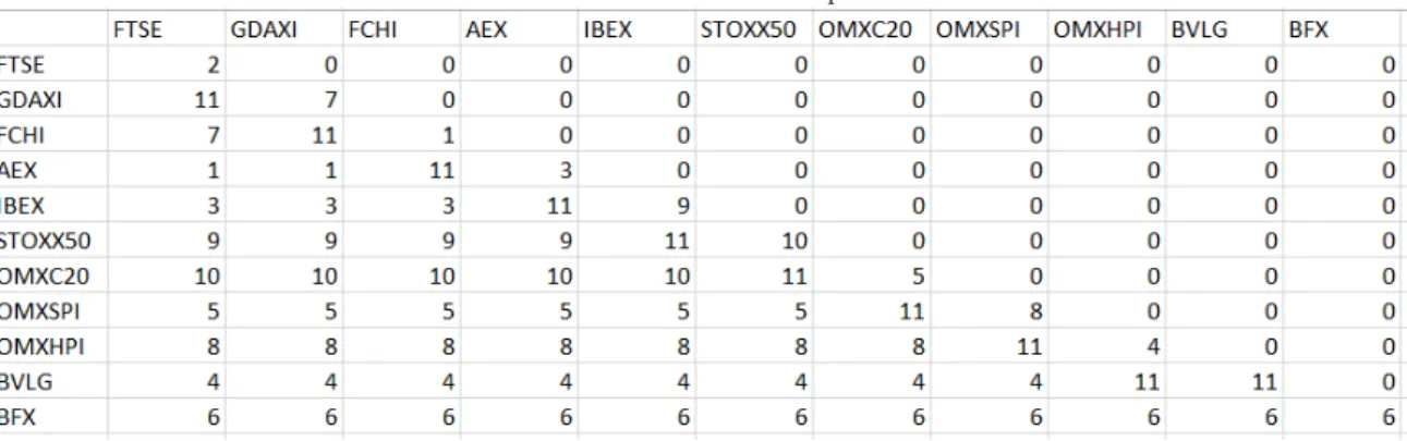
The pre-GFC C-Vine copula specication matrix is displayed in Table 5 below. It can be seen from the top and bottom of the rst column in Table 5 that in the pre-GFC period the strongest correlations are between the FTSE and Belgian Index BFX. The BFX remains at the bottom across all columns in the last row of Table 5.
Table 5: Pre-GFC C-Vine Copula Structure
Table 6: Pre-GFC C-Vine Copula Specication Matrix
From Table 5, it can be seen that the strongest individual correlations in the pre-GFC period, are between the FTSE at the top of the rst column, BFX in the nal row, and the individual diagonal entries starting with the FTSE at the top of the rst column, which dene the edges. The FTSE is correlated with BVLG (security 11), then conditioned by its relationship with OMXHPI (security 8), the Helsinki exchange index, then OMXSPI (security 5), the Stockholm index, then OMXC20 (security 3), the Copenhagen index, and so on. It can also be seen in Table 5 that C Vines are less exible in that the same security number can usually be seen to appear across the rows. This means that it is always appearing in the nodes at that level in the tree. R Vines are more exible and do not have this requirement. Later in the paper, we will concentrate on the results of the R Vine analysis.
Table 6 shows which copula are tted to capture dependencies between the various pairs of indices. At the bottom of column 1 in Table 6 we can see that number 2 copula, the Student t copula is applied, to capture the dependency between FTSE and BFX, and then it is conditioned by the relationship with BVLG but this relationship uses a Frank copula (5), and so forth. All 6 categories of copula are used in Table 6 but the Student t copula appears most frequently in the table, followed by the Frank copula, the Gaussian copula, the Clayton copula and nally the Joe copula and the Gumbel copula appear once each.
Table 7: Pre-GFC C-Vine Copula Parameter Estimates
It can be seen in Table 7 in the entries in the bottom row that there are strong positive dependencies between subsets of the markets concerned. The entry in the bottom of the rst column shows the strong positive dependency between the FTSE and BFX. All the entries in the bottom row of Table 7 are strongly positive. We can see in the rst column, that once we have conditioned the FTSE on its
4.3 GFC period 11 relationships with the markets in the bottom half of the column it is strongly positively related to the STOXX50. Not all the dependencies indicated in Table 7 are positive though, and there are 11 cases of negative co-dependency, once the relationship across other nodes has been taken into account.
Table 8 shows the second set of parameters, in cases where one is needed, for example the Student t copula.
Table 8: Pre-GFC C-Vine Copula Second Parameter Estimates
Table 9 shows the tau matrix for the C Vine copulas in the pre-GFC period.
Table 9: Pre-GFC C-Vine Copula Tau matrix
The bottom row of Table 9 captures the strongest dependencies between the pairs of markets, as represented by their respective indices.
A key concern in this paper is the issue of how dependencies have changed as a result of the GFC? 4.3. GFC period
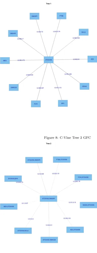
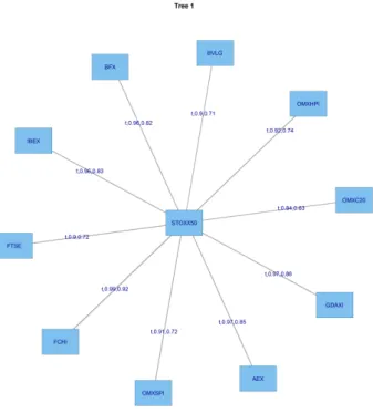
Figure 7 shows tree 1 for C-Vine copula estimates in the GFC period, and Figure 8 shows tree 2 for the same period.
Figure 7: Results-C-Vine Tree-1 GFC
Figure 8: C-Vine Tree 2 GFC
We are interesting in examing whether the major nancial shock which constituted the GFC caused a noticeable change in dependencies?
4.3 GFC period 13
Table 10: GFC C-Vine Copula Structure
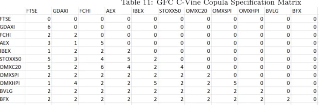
Table 11 depicts the copulas chosen to capture dependency relationships during the GFC period.
Table 11: GFC C-Vine Copula Specication Matrix
A comparison of the entries in Table 11, the copula specication matrix for the GFC, with those in Table 6, the pre-GFC copula specication matrix, reveals that there is much less us of Gaussian copulas, 3 in Table 11, compared with 11 in Table 6. There is now a much greater use made of the Student t copula, on 36 occasions in Table 11, compared with 18 in Table 6. The use of the Gumbel copulas has increased from 1 to 4 occasions and the Clayton copula is only used on 2 occasions compared with 5 pre-GFC. The use of the Frank copula has declined from 15 to 6, whilst the Joe copula, now makes 2 appearances compared to 1 pre-GFC. The massive expansion of the use of the Student t copula, together with the other changes mentioned, is consistent with greater weight being placed on the tails of the distribution durng the GFC period.
The dependencies are captured in the Tau matrix shown in Table 12.
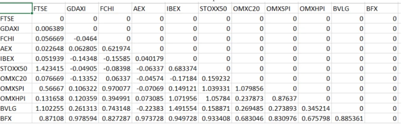
Table 12: GFC C-Vine Copula Tau matrix
A comparison of the values in Table 12, the tau matrix for the GFC, with those in Table 9, the tau matrix for the pre-GFC period, reveals that the relationships have become more pronounced. If we look at the dependencies in the bottom row of Table 12, in 7 from the total of 10 cases the dependencies have increased. It is also true that there has also been a marginal increase in negative dependencies, from 10 pre-GFC to 12 during the GFC, but the values of these are of a low order. The picture that emerges from Table 12 is one of an increase in dependencies between these major European stock markets during an economic down-turn.
4.4. Post-GFC period
We will now turn our attention to the post-GFC period. In the case of the European markets, this is likely to be less-clear cut, given that it was characterised by economic turmoil related to the subsequent post-GFC European Sovereign debt crisis. Figure 9 displays the rst tree post-GFC, and Figure 10 the second tree.
Figure 9: Results-C-Vine Tree-1 post-GFC
4.4 Post-GFC period 15 Table 13 shows the post-GFC C-Vine copula structure, and Table 14 the post-GFC C-Vine Copula Specication Matrix.
Table 13: Post-GFC C-Vine Copula Structure
Table 14: Post-GFC C-Vine Copula Specication Matrix
It can be seen in Table 14 that there is a marked change in the type of copula used to capture dependencies in the post-GFC period. The use of the Gaussian copula has risen from 3 during the GFC period to 10 in the post-GFC period, and the application of the Student t copula has dropped from 36 during the GFC to 24 in the post GFC period, whilst the use of the Clayton copula in the post-GFC period rises to 8 from 2 in the GFC period. The Gumbel copula is used on 6 occasions, whilst the Frank copula appears only 5 times, compared with 15 in the pre-GFC period. Finally, the Joe copula, is made use of on 1 occasion. The increase in the use of the Gaussian copula and the reduction in the use of the Student t copula suggests there is much less emphasis on the tails of the distributions in the post-GFC period.
The post-GFC tau matrix is shown in Table 15.
Table 15: Post-GFC C-Vine Copula Tau matrix
The structure of dependencies that emerges in Table 15 is quite complex when compared to those of the GFC period. In the bottom row the positive dependencies captured in the tau statistics have
increased in 7 of the total of 10 cases. In the GFC period there were 12 negative tau coecients in the matrix, where as in the post-GFC period this number has reduced to 10. Thus, the broad picture that emerges in the post-GFC period, based on the use of C-Vine copulas, is that overall dependencies increased in the post-GFC period across the major European markets, in association with their experience of the European Sovereign debt crisis. The greater use of Gaussian copulas and the reduction in the use of Student t copulas in this period, suggests that tail behaviour was less important.
We now switch to the more exible R-Vine framework to compare the two approaches. 5. R Vine copulas
5.1. The pre-GFC period
5.1 The pre-GFC period 17
Figure 12: Results-R-Vine Tree-3 pre-GFC
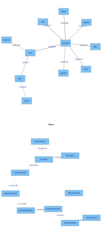
It can be seen in Figures 11 and 12 above that the R Vine structure is more exible. Tree 1 shows that a sub-group of the European markets are linked together; namely the Portuguese (BVLG), Brussels (BFY), the French (FCHI) and the Danish (OMXC20), they are then linked to the European Index (STOXX50). The other markets; Amsterdam (AEX), Germany (GDAXI), Stockholm (OMXSPI), Spain (IBEX), the UK (FTSE), and Helsinki (OMXHPI), have the strongest co-dependency with the European Index (STOXX50). This is also apparent in Tables 16 and 17 which show the general dependence relationships.
5.1 The pre-GFC period 19
Table 16: Pre-GFC R-Vine Copula Structure
Table 17: Pre-GFC R-Vine Copula Specication Matrix
Table 17 shows the types of copulas tted in the empirical analysis.
The advantage of the use of R Vines is apparent in Table 17. Complex patterns of dependency can be readily captured. It can be seen that at dierent dependencies conditioned across the same node six dierent copulas are used. For example, in column 1 the rst copula used is the Clayton copula (no 3), followed by the Frank copula (no 5) for a couple of levels, then the Joe Copula (no 6), the Frank copula (no 5), two cases of the Gaussian (no 1), then the Gumbel (no 4), then the Frank copula again, and nally, the Student t (no 2). This variety of usage is apparent across Table 15 at various levels in the tree structures used to capture dependencies. The bottom row consists entirely of Student t copulas.
The copulas used to capture co-dependencies are dierent from the pre-GFC period C-Vine analysis. In that case, illustrated in Table 5; 11 Gaussian, 18 Student t copulas, 5 Clayton copulas, I Gumbel, 15 Frank copulas, and 1 Joe Copula were used. By contrast, in Table 17, 11 Gaussian, 18 Student t, 9 Clayton, 3 Gumbel, 12 Frank and 1 Joe copula are used. This follows, given that dierent co-dependencies are captured in the tree because there are not constraints on the pairings in R Vine copulas.
In the interests of brevity the details of the parameters estimated are not tabulated but the tau matrix, is shown in Table 18.
The entries in Table 18 for R-Vines can be contrasted with those in Table 9 for C-Vines. Once again, given the nature of the analysis, the strongest dependencies between the various indices are captured by the entries in the bottom row of the table. Overall, the picture of dependencies is similar to those captured by the C-Vine analysis. The biggest change is in the rst column of Table 18 in that the relationships between the FTSE and STOXX50, OMXC20 and OMXSPI have now become negative, but it has to be born in mind that the relationship is now conditioned on the much stronger relationship between the FTSE and BFX.
5.2. R-Vines GFC
5.2 R-Vines GFC 21
Figure 13: Results-R-Vine Trees-1 and 2 GFC
The trees shown in Figure 13 indicate that dependencies have changed because of the inuence of the GFC and the FTSE is now linked via the French FCHI to the STOXX50, whilst the OMXC20 and OMXSPI are now linked via the FCHI to the STOXX50. Previously, in the pre-GFC period the BVLG and the BFX were linked by the FCHI, but this is no longer the case.
Table 19: GFC R-Vine Copula Specication Matrix
Table 19 once again suggests the importance of capturing tail risk in nancial and economic downturns plus the importance of fat-tailed distributions. Only 4 Gaussian copulas are applied in Table 19, where as the Student t copula dominates, being used on 38 occasions. There are 2 applications of the Clayton copula, 5 of the Gumbel and 4 of the Frank, whilst the Joe copula is used on 1 occasion.
Table 20 provides details of the tau matrix for the GFC period.
Table 20: GFC R-Vine Copula Tau matrix
The change in dependencies in the R-Vine analysis following the GFC is complex and dicult to interpret in a clear-cut fashion. In terms of the dependencies captured in the bottom row of Table 20, 5 show an increase in their values, compared with the pre-GFC entries in Table 18 but 5 also show a decrease. In terms of the whole matrix, the number of negative entries in Table 20 is 10, the same as the number in Table 18, but because of complex changes in patterns of dependencies, they now occur at predominantly dierent positions in the matrix.
We will therefore move on to the post-GFC R-Vine analysis. 5.3. Post-GFC R-Vines
5.3 Post-GFC R-Vines 23
Figure 14 reveals that the relationships between the markets have changed in a complex manner in the post GFC period. It can be seen in tree 1 that the FTSE is now linked to the STOXX50 via the Dutch and French Indices. The Finnish, Danish and Swedish markets are also linked via the Durch and French markets to the STOXX50. The German and Spanish markets have individual links to the STOXX50, whilst the Portuguese market is linked via the Belgian index to the STOXX50. Table 21 shows the types of copulas used to map dependencies in the post-GFC period.
Table 21: Post-GFC R-Vine Copula Specication Matrix
The Gaussian copula is used on 9 occasions whilst the Student t copula again dominates with 25 entries in Table 21, a considerable reduction on the 38 times it was applied during the GFC period. The Clayton copula appears 4 times, the Gumbel on 2 occasions. Greater use is made of the Frank copula, which appears 8 times, and nally the Joe copula is used on 4 occasions.
The tau dependency matrix is shown in Table 22.
Table 22: Post-GFC R-Vine Copula Tau matrix
The tau matrix in Table 22 shows that dependencies have again changed in a complex manner in the post-GFC period which coincides with the European Sovereign debt crisis. The large dependencies in the bottom row have increased in 6 of the 10 cases in the post-GFC period. However, there are 12 cases of negative relationships in Table 22 as opposed to 8 in Table 20 representing the GFC period. These changes are interesting but do not give a direct indication of the usefulness of R-Vine modelling. We therefore illustrate an empirical application of the approach in the next section which features a Value at Risk, (VaR) analysis.
6. An empirical application 6.1. Empirical Example
We have used C-Vine and R-Vine Copulas to map dependence structures between some of the major European markets. These, in turn, can be used for portfolio evaluation and risk modelling. The R-Vine approach potentially gives better results than usual bivariate copula approach given that the copulas selected via Vine copulas are more sensitive to the asset's return distributions.
The co-dependencies calculated by R-Vine copulas can be used for portfolio Value at Risk quantica-tion. We construct an equally weighted portfolio of the eleven market indices to explore the use of Vine
6.1 Empirical Example 25 copulas in modelling VaR using a portfolio example. The data used for this part of the analysis is from 3-Jan-2010 to 31-Dec-2011 with a total of 504 returns per asset, the ten selected assets in the portfolio are our ten European market indices. We use a 250 days moving window to generate 51 forecasts using 300 returns per asset. The time period for VaR forecast data is 24-10-2011 to 2011-12-30. The main steps of the approach are as outlined below:
1. Convert the data sample to log returns. 2. Select a moving window of 250 returns.
3. Fit GARCH(1,1) with Student-t innovations to convert the log returns into an i.i.d. series. We t the same GARCH(1,1) with student-t in all the iterations to maintain uniformity in the method, and this approach also makes the method a little less computationally intensive.
4. Extract the residuals from Step-3 and standardize them with the Standard deviations obtained from Step-3.
5. Convert the standardized residuals to student-t marginals for Copula estimation. The steps above are repeated for all the 10 stocks to obtain a multivariate matrix of uniform marginals.
6. Fit an R-Vine to the multivariate data with the same copulas as used in Section-1.
7. Generate simulations using the tted R-Vine model. We generate 1000 simulations per stock for forecasting a day ahead VaR.
8. Convert the simulated uniform marginals to standardized residuals.
9. Simulate returns from the simulated standardized residuals using GARCH simulations. 10. Generate a series of simulated daily portfolio returns to forecast 1% and 5% VaR. 11. Repeat step 1 to 10 for a moving window.
The approach above results in VaR forecasts which whilst not dependent in time have the advantage of being co-dependent on the stocks in the portfolio. We use this approach as a demonstration of a practical application of the information about co-dependencies captured by the exible Vine Copula approach applied to construct VaR forecasts. Figure 15 plots the 1% and 5% VaR forecasts along with original portfolio return series obtained from the method. The plot shows that the VaR forecasts closely follow the daily returns with few violations.
Figure 15: R-Vine Forecasts
Table 23 below gives the results from Unconditional Coverage (Kupiec) and Conditional Coverage (Christoersen) (Christoersen, 1998 and Christoersen, Hahn and Inoue, 2001) which are based on the number of VaR violations compared to the actual portfolio returns. According to the results in the table both the tests accept both the 1% and 5% VaR models for the forecasting period, given that they fail to reject the null hypothesis.
Table 23: VaR Back-Test Results
expected.exceedactual.exceeduc.H0 uc.LRstat uc.critical uc.LRp uc.Decision cc.H0 cc.LRstat cc.critical cc.LRp cc.Decision 5% 2 1 Correct
Ex-ceedances
1.276879991 3.841458821 0.258479955 Fail to Reject H0 Correct Ex-ceedances & Indepen-dent 1.317699151 5.991464547 0.517446275 Fail to Reject H0 1% 0 0 Correct Ex-ceedances
1.025134257 3.841458821 0.311304237 Fail to Reject H0 Correct Ex-ceedances & Indepen-dent 1.025134257 5.991464547 0.598956006 Fail to Reject H0
*P-Value>0.05 (95% condence) results in the acceptance of the null hypothesis.
7. Conclusion
In this paper we used the recently developed R Vine copula methods (see Aas et al. (2009), Berg and Aas (2009), Min and Czado (2010) and Czado et al. (2011)) to analyse the changes in the co-dependencies of ten European stock market indices and the composite STOXX50 index for three periods spanning the GFC: pre-GFC (Jan 2005- July 2007), GFC (July 2007-Sep 2009) and post-GFC periods (Sep 2009 - Dec 2011). The results suggest that the dependencies change in a complex manner, and there is evidence of greater reliance on the Student t copula, in the copula choice within the tree structures, for the GFC period, which is consistent with the existence of larger tails to the distributions of returns. One of the attractions of this approach to risk-modelling is the exibility available in the choice of distributions used to model co-dependencies. We demonstrate the calculation of portfolio VaR on the basis of these dependency measures and the method appears to work well on the basis of coverage ratio tests.
The main limitation is the static nature of the approach and dynamic applications are in the process of development. (See for example, Breckmann and Czado (2012)).
Acknowledgement: For nancial support, the authors wish to thank the Australian Research Council. The third author would also like to acknowledge the National Science Council, Taiwan,
and the Japan Society for the Promotion of Science. The authors thank the reviewers for
27 References
[1] Aas, K., C. Czado, A. Frigessi and H. Bakken (2009) Pair-copula constructions of multiple dependence, Insurance, Mathematics and Economics, 44, 182198.
[2] Allen, D. E., A. Ashraf, M. McAleer, R.J. Powell, and A.K. Singh, (2013) Financial de-pendence analysis: applications of vine copulas, Statistica Neerlandica, 87, 4, 403-435. [3] Bedford, T. and R. M. Cooke (2001) Probability density decomposition for conditionally
dependent random variables modeled by vines, Annals of Mathematics and Articial Intel-ligence 32, 245-268.
[4] Bedford, T. and R. M. Cooke (2002) Vines - a new graphical model for dependent random variables, Annals of Statistics 30, 1031-1068.
[5] Berg, D., (2009) Copula goodness-of-t testing: an overview and power comparison, The European Journal of Finance, 15:675701.
[6] Berg, D., and K. Aas, (2009) Models for construction of higher-dimensional dependence: A comparison study, European Journal of Finance, 15:639659.
[7] Brechmann, E. C., C. Czado, and K. Aas, (2012) Truncated regular vines and their appli-cations, Canadian Journal of Statistics 40 (1), 68-85.
[8] Brechmann, E.C. and C. Czado (2013), Risk Management with High-Dimensional Vine Copulas: An Analysis of the Euro Stoxx 50, Statistics and Risk Modeling, 30(4), 307-342. [9] E.C. Brechmann, C. Czado and S. Paterlini (2014), Flexible Dependence Modeling of Operational Risk Losses and Its Impact on Total Capital Requirements, Journal of Banking and Finance, 40, 271-285.
[10] Brechmann, E.C., and U. Schepsmeier, (2012) Modeling dependence
with C- and D-vine copulas The R-package CDVine,
http://cran.r-project.org/web/packages/CDVine/vignettes/CDVine-package.pdf
[11] Brechmann, E. C., and C. Czado (2012) COPAR - multivariate time-series modelling using the COPula AutoRegressive model, Working Paper, Faculty of Mathematics, Technical University of Munich.
[12] Chollete, L., Heinen, A., and A. Valdesogo, (2009) Modeling international nancial returns with a multivariate regime switching copula, Journal of Financial Econometrics, 7:437480. [13] Christoersen, P., (1998) Evaluating Interval Forecasts, International Economic Review,
39, 841862.
[14] Christoersen, P., J. Hahn, and A. Inoue, (2001) ``Testing and Comparing Value-at-Risk Measures'', Journal of Empirical Finance, 8, 325342.
[15] Cooke, R.M., H. Joe and K. Aas, (2011) Vines Arise, chapter 3 in DEPENDENCE MOD-ELING Vine Copula Handbook, Ed. D. Kurowicka and H. Joe, World Scientic Publishing Co, Singapore.
[16] Czado, C., U. Schepsmeier, and A. Min (2011) Maximum likelihood estimation of mixed C-vines with application to exchange rates. To appear in Statistical Modelling.
[17] Czado, C., E.C. Brechmann and L. Gruber (2013) Selection of Vine Copulas, in P. Ja-worski, F. Durante and W. K. Härdle (Eds.), Copulae in Mathematical and Quantitative Finance: Proceedings of the Workshop Held in Cracow, 10-11 July 2012, Springer.
[18] Dimann, J., E. C. Brechmann, C. Czado, and D. Kurowicka (2012) Selecting and es-timating regular vine copulae and application to nancial returns, Submitted preprint. http://arxiv.org/abs/1202.2002.
[19] Dissman, J.F. (2010) Statistical Inference for Regular Vines and Application, Thesis, Tech-nische Universitat Munchen, Zentrum Mathematik.
[20] Heinen, A. and A. Valdesogo (2009) Asymmetric CAPM dependence for large dimen-sions: the canonical vine autoregressive model, CORE discussion papers 2009069, Univer-site catholique de Louvain, Center for Operations Research and Econometrics (CORE). [21] Joe, H., (1996) Families of m-variate distributions with given margins and m(m- 1)/2
bivariate dependence parameters. In L. Rüschendorf and B. Schweizer and M. D. Taylor, editor, Distributions with Fixed Marginals and Related Topics.
[22] Joe, H. (1997) Multivariate Models and Dependence Concepts. Chapman & Hall, London. [23] Joe, H., Li, H., and A. Nikoloulopoulos, (2010) Tail dependence functions and vine copulas,
Journal of Multivariate Analysis, 101(1):252270.
[24] Kullback, S. and R.A. Leibler, (1951) On information and suciency, The Annals of Mathematical Statistics, 22(1):7986.
[25] Kupiec, P., (1995) ``Techniques for verifying the accuracy of risk measurement models'', Journal of Derivatives 3, 73-84.
[26] Kurowicka, D., (2011) Optimal truncation of vines, In D. Kurowicka and H. Joe (Eds.), Dependence Modeling: Handbook on Vine Copulae. Singapore: World Scientic Publishing Co.
[27] Kurowicka D. and R.M. Cooke, (2003) A parametrization of positive denite matrices in terms of partial correlation vines, Linear Algebra and its Applications, 372, 225251. [28] Kurowicka, D. and R. M. Cooke, (2006) Uncertainty Analysis with High Dimensional
Dependence Modelling, Chichester: John Wiley.
[29] Mendes, B. V. d. M., M. M. Semeraro, and R. P. C. Leal, (2010) Pair-copulas modeling in nance, Financial Markets and Portfolio Management 24, 193-213.
[30] Min, A., and C. Czado, (2010) Bayesian inference for multivariate copulas using pair-copula constructions, Accepted for publication in Journal of Financial Econometrics.
[31] Morales-N´apoles, O., R. Cooke, and D. Kurowicka (2009) About the number of vines and regular vines on n nodes, Submitted to Linear Algebra and its Applications.
[32] Nelsen, R., (2006) An Introduction to Copulas, Springer, New York, 2nd edition.
[33] Patton, A. J., (2009) Copula based models for nancial time series, in: Handbook of Financial Time Series. pp. 767-785
[34] Prim, R. C., (1957) Shortest connection networks and some generalizations, Bell System Technical Journal, 36:13891401.
[35] Schirmacher, D. and E. Schirmacher, (2008) Multivariate dependence mod-eling using pair-copulas, Technical report, Society of Actuaries: 2008 En-terprise Risk Management Symposium, April 14-16, Chicago. Available from: http://www.soa.org/library/monographs/other-monographs/2008/april/ 2008-erm-toc.aspx
[36] Sklar, A., (1959) Fonctions de repartition a n dimensions et leurs marges, Publications de l'Institut de Statistique de L'Universite de Paris 8, 229-231.
[37] Smith, M., Min, A., C. Czado, C., and C. Almeida, (2010) Modeling longitudinal data using a pair-copula decomposition of serial dependence, In revision for the Journal of the American Statistical Association.
[38] Vuong, Q. H., (1989) Likelihood ratio tests for model selection and non-nested hypotheses, Econometrica, 57:307333.