Constraint Optimization for
Highly Constrained Logistic Problems
Maria Kinga Mochnacs
Meang Akira Tanaka
Anders Nyborg
Rune Møller Jensen
IT University Technical Report Series
TR-2007-2008-104
Copyright c
2007,
Maria Kinga Mochnacs
Meang Akira Tanaka
Anders Nyborg
Rune Møller Jensen
IT University of Copenhagen
All rights reserved.
Reproduction of all or part of this work
is permitted for educational or research use
on condition that this copyright notice is
included in any copy.
ISSN 1600–6100
ISBN 978-87-7949-163-2
Copies may be obtained by contacting:
IT University of Copenhagen
Rued Langgaards Vej 7
DK-2300 Copenhagen S
Denmark
Telephone: +45 72 18 50 00
Telefax:
+45 72 18 50 01
Abstract
This report investigates whether propagators combined with branch and bound al-gorithm are suitable for solving the storage area stowage problem within reasonable time. The approach has not been attempted before and experiments show that the implementation was not capable of solving the storage area stowage problem effi-ciently. Nevertheless, the report incorporates a detailed analysis of the problem, acts as a valuable basis for comparing the quality of alternative approaches and reveals the properties of the solution space.
Contents
1 Introduction 1
2 Background 3
2.1 Constraint satisfaction problems . . . 3
2.2 Search algorithms . . . 5
2.3 Constraint optimization problems . . . 6
2.3.1 Branch and Bound . . . 7
2.3.2 Model of a constraint optimization problem . . . 8
3 The Storage Area Stowage Problem 11 3.1 Background . . . 11
3.2 Formal definition of SASP . . . 16
4 Evaluating CSP representations of SASP 25 4.1 Pruning operations . . . 25 4.2 Container-model . . . 27 4.3 Slot-model . . . 29 4.4 Cell-model . . . 30 4.5 Conclusion . . . 32 5 CSP representation of SASP 35 5.1 Variables . . . 35 5.2 Domains . . . 35
5.3 Additional constraints and pruning operations . . . 37
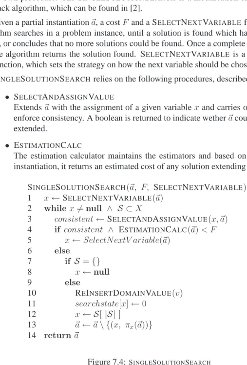
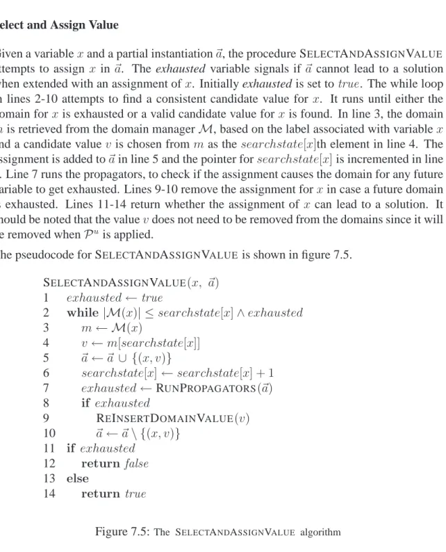
5.5 Early termination criteria . . . 42 5.6 Correctness of propagators . . . 42 6 Estimation 47 6.1 Overstowage Bounding . . . 47 6.2 Emptystack Bounding . . . 50 6.3 Wastedspace Bounding . . . 54 6.4 Reefer Bounding . . . 55 7 Implementation 57 7.1 Fundamental concepts . . . 57 7.2 Representing data . . . 67 7.3 Algorithm . . . 68 7.4 Search . . . 68
7.4.1 Single solution search . . . 69
7.4.2 Depth First Branch and Bound . . . 72
8 Experiments 77 8.1 Test components . . . 77 8.1.1 Test data . . . 77 8.1.2 Search . . . 78 8.1.3 Measurements criteria . . . 81 8.2 Propagator improvements . . . 81
8.2.1 Searching for a single solution . . . 82
8.2.2 Traversal of the search space . . . 83
8.3 Estimators . . . 85
8.3.1 Traversal of the search space . . . 85
8.4 Lazy Estimation . . . 86
8.4.1 Traversal of the search space . . . 86
8.5 Approximation . . . 91
8.5.1 Traversal of the search space . . . 91
8.6.1 Searching for a single solution . . . 93
8.7 Profiling . . . 95
8.8 Solution discoveries . . . 98
8.8.1 Traversal of the search space . . . 98
8.9 Conclusion on experiment . . . 101 9 Conclusion 103 A Program organization 109 B Informal description 115 C Pseudo code 119 C.1 Evaluation . . . 119 C.1.1 Overstowage Evaluation . . . 119 C.1.2 Wastedspace Evaluation . . . 120 C.2 Estimation . . . 121 C.2.1 Overstowage Estimation . . . 121 C.2.2 Wastedspace Estimation . . . 124
C.3 Domain management function . . . 127
C.4 Propagators examples . . . 128
C.4.1 Uniqueness . . . 128
Chapter 1
Introduction
Containerized transport in vessels traveling overseas is a field in rapid growth. As the trade increases, pressure is put on shipping companies to lower the cost of their transportation services. For that reason, there is an interest in the industry for developing algorithms, which can help placing containers efficiently aboard a vessel, respecting safety require-ments and optimizing logistic criteria. Viewed from an academic perspective the problem has some interesting properties, as it contains subproblems, which have been proven to be NP-hard [1].
Placing containers on a vessel can be regarded as a combinatorial problem. The size of the combinatorial space can be roughly estimated as a permutation of placing a unique con-tainer for each slot available. Since a bay may accommodate up to 200 20-foot concon-tainers, the combinatorial space is immense, making it a very hard combinatorial problem.
One typical approach used within the field of operations research is to solve the problem by using integer programming. However nonlinear constraints cannot be modeled properly by the usage of integer programming. Consequently alternative approaches have to be considered.
In this report, an in depth study is given of the storage area stowage problem, which is a constraint optimization problem, consisting of arranging a set of containers below deck within a bay of a vessel. The safety requirements and logistic criteria are divided into hard and soft constraints respectively. A weight has been defined for each soft constraint to identify the importance of fulfilling each logistic criteria. Due to the ability of modeling nonlinear constraints in a simple fashion, functions known as propagators has been cho-sen to reprecho-sent the constraints within the problem The chocho-sen algorithm for solving the problem is branch and bound, described by [2] as: ”the most commonly known algorithm for solving constraint optimization problems”. The algorithm and choice of representation was selected based on the fact that no research within the field of containerized transport overseas exists, relying on this combination to solve the storage area stowage problem. The goal is that the research provided in this report will serve as a first step, in uncovering some
of the strengths and weaknesses by using a Constraint Satisfaction Problem(CSP)-model and branch and bound for solving the storage area stowage problem.
The issues which, this report would like to address is as follows:
Can backtrack combined with a CSP-Model find a solution within reasonable time for the storage area stowage problem.
Can branch and bound combined with a CSP-Model find an optimal solution within reasonable time for the storage area stowage problem.
Several task had to be formulated in order to answer the above issues. The first tasks, is to get a thorough understanding by formulating a mathematical model of the problem. The second task is to find a suitable CSP-Model by considering different candidate models, evaluate each of these, and select the most suitable candidate. The third tasks is to conduct experiments on the developed implementation and analyze the results.
Document outline
In chapter 2, the theoretical background of the report is established. Based on the the-ory and an informal problem description, the problem is formalized into a mathematical model in chapter 3. Three candidate CSP-Models are suggested based on an analysis of the formalized model in chapter 4. Chapter 5 formalize the chosen CSP-Modeland the formal-ization of the estimators are presented in chapter 6. Implementation of the CSP-Modeland search algorithms are represented in chapter 7. Based on the implementation, experiments are performed to cover different aspects of the search space and implementation in chapter 8. Chapter 9 concludes the report with some suggestion of what can be done in future.
Chapter 2
Background
This chapter provides a brief explanation of different constraint processing concepts used in the report.
2.1
Constraint satisfaction problems
Constraint satisfaction problems, or CSPs, are mathematical problems that typically
in-volve finding out how to assign a discrete set of variables under certain constraints. Many solutions may actually satisfy the constraints of the problem.
For many hard constraint satisfaction problems, no algorithm has been discovered to solve the problem efficiently yet and some have been proved to be NP-hard. Solving these combi-natorial problems is done by searching in the solution space, which is typically exponential in the size of the problem. A systematic search of the search space ensures that all candidate solutions are considered and the optimal one is found with certainty.
A constraint network is a model of a CSP that consists of a finite set of variables, a finite set of domains, and a finite set of constraints. A variable is a value holder for an entity of the problem. Each variable has its own domain that lists the possible values the variable can take. A constraint is a relation defined on a subset of variables that represents simultaneous legal assignments of the variables. A constraint can be specified explicitly by the list of satisfying tuples, or implicitly by a formula that characterizes the constraint.
An instantiation is the assignment of some subset of variables with some value from the domain of each variable. When all variables are assigned, the instantiation is said to be
complete. Otherwise the instantiation is said to be partial. An instantiation is consistent, if
it satisfies all of the constraints, whose scopes have no uninstantiated variables.
A valid solution of the constraint network is a consistent complete instantiation of all of its variables. An unsatisfiable problem does not have any solutions.
Constraint propagation
Searching for solutions can be viewed as traversing a search space, where the task is to reach a state, where all variables have been assigned with a legal value from their domain. Moving from one state to another state in the search space implies assigning or unassign-ing variables. The search space of the problem can be considerably larger than the solution space, potentially containing many inconsistent instantiations in respect to the given prob-lem. Consequently, searching for solutions can be very inefficient. An approach is to tighten the search space by formulating an equivalent but more explicit model.
In general, the more explicit the model is, the more restricted the search space will be, mak-ing search more effective. When any consistent instantiation of a subset of variables can be extended to a consistent instantiation of all the variables, the model is said to be globally
consistent. Having a model, which is globally consistent, makes it straightforward to find
solutions, since any value chosen for any variable will lead to a solution. However com-puting a globally consistent model is intractable for sufficiently large problems. Instead, transforming a model into an approximation of a global consistent model may be preferable due to the lower computation cost.
Constraint propagation is the process of transforming a model into a tighter one. The
tightening process can be done during the search itself, by inferring new knowledge using
local consistency enforcing algorithms that perform a bounded amount of constraint
infer-ence during each iteration, such as arc or path consistency. A local consistency property is defined regardless of the domains or constraints of the CSP problem.
Another approach to do constraint propagation is rules iteration. Rules iteration tightens a model by iteratively applying reduction rules. A reduction rule or a propagator is a decreasing function that rules out domain values, which will not appear in a solution. A propagator depends on one or more input variables and changes the domain of one or more
output variables. The assignment of an input variable triggers the propagator. Propagators
can be seen as an actual implementation of the constraints themselves. When assigning one variable a specific value, the set of propagators remove values from the domain of the uninstantiated variables enforcing consistency with the newly instantiated variable.
A one-to-one relationship does not necessarily exists among the set of constraints and the set of propagators. The problems nature may imply that it is easier to construct several propagators that jointly implement a specific constraint. When a combination of several propagators together implement a given constraint, the propagators that the combination consists of is said to contain the constraint.
Example 2.1 One of the constraints within the storage area stowage problem is that a 20-foot container cannot be stacked on top of a 40-20-foot container. One approach is to divide the constraints into two propagators: One, which ensures that no 40-foot containers can be placed below a 20-foot container and one, which ensures that no 20-foot container can
be placed on top of a 40-foot.
For details of rules iteration and how a propagation engine works, refer to [3].
2.2
Search algorithms
The goal of a search algorithm is to find solutions to the CSP or conclude that the problem is unsatisfiable. Traversing the search space can be based on different strategies, each strategy resulting in a family of search algorithms. The search family this report considers is the backtrack search family.
Backtrack search algorithms belong to the family of systematic search and, as a conse-quence, are guaranteed to be complete. The completeness is attained by viewing the search space as a tree, where each node in the tree is an instantiation of a single variable and each branch is a possible assignment for that particular variable. The depth of the tree is deter-mined by the number of variables and consequently the paths, from the root to a leaf node in the tree, are complete instantiations. The starting point, where all backtrack algorithms originate from, is the naive backtrack algorithm, which can be thought of as an algorithm which performs a depth first traversal of the tree, until a solution is found. If some variable along the path towards the leaf node results in an inconsistent partial instantiation, a back-track occurs. Backback-tracking is the process, where the assignment of a previously assigned variable is reconsidered. Traversing the tree is clearly exponential in time in the worst case and is not practical for too large problems. Therefore, many variations of the naive backtrack algorithm, which tries to improve search time, have been suggested.
This report considers two members of the backtrack family: Forward checking and Dy-namic Variable Forward Checking (DVFC). The motivation for choosing forward check-ing, is that the problem contains properties, which makes the algorithm suitable for finding optimal solutions efficiently along a static variable order. The DVFC has been chosen based on previous experience of being an algorithm, which could find a solution fast, since being based on the forward checking approach of pruning, ensures that the branching factor of the next variable to be instantiated is at a minimum [4].
Current variable is the variable, which the search algorithm currently is attempting to find
an assignment for. The nodes of the search tree represent the current variable of a specific stage in the search.
Candidate value is any possible value an uninstantiated variable can be assigned to. In
respect to the search tree the branches of a node are candidate values.
Current instantiation is the assignments that has been done until so far in the search. The
path from the root of the search tree down to current variable is the current instantiation.
variable. The set of nodes along any path from the current variable is the future variables.
Forward Checking
Forward checking is a simple improvement to naive backtracking. The principle is to prune domain values from future variables, that are inconsistent with the currently instan-tiation. Given a CSP-Model, where the constraints are represented with propagators, for-ward checking is achieved in a straightforfor-ward way: Whenever a variable is assigned, all propagators that specify the variable as input are applied. This guarantees that the current instantiation is consistent with any assignment of some future variable. Forward checking is superior compared to naive backtracking, in that it ensures that thrashing is avoided at an earlier stage of a given instantiation.
DVFC
DVFC is a heuristic based on the forward checking strategy that takes into account the benefits of variable orderings, which produces a small search space. DVFC determines the variable ordering dynamically, during search. It relies on the fail-first heuristic, by se-lecting the variable, which is most likely to restrict the search space as early as possible. By considering the variables that most likely restrict the search space as early as possible, DVFC strengthens the benefits of forward-checking look ahead by being able to detect dead ends as soon as possible considering the amount inference. All other factors being equal, the variable with the smallest number of viable values in its current domain, will have the fewest subtrees rooted at those values, and therefore the smallest search space below it. For a thorough presentation of backtrack variations and their standard implementation refer to [2].
2.3
Constraint optimization problems
For some problems, candidate solutions must be ranked in terms of quality to some given criteria. In this case, constraint problems are optimization problems or COPs. The quality is described by an objective or cost function and the goal is to find a solution with as high quality as possible, in other words a solution with an optimal objective function value. In case the objective function has to be minimized, a minimization problem is considered, otherwise a maximization problem is considered.
A CSP-Model augmented with a cost function provides a framework to model a COP. Typ-ically, the cost function is a weighted sum of several cost components. A cost component
is a problem-dependent real value function defined on a subset of variables. The cost com-ponents are also referred to as soft constraints, while the constraints of the problem are referred to as hard constraints.
An optimal solution for a minimization problem is any valid solution which has the lowest cost amongst all valid solutions.
For a detailed description of COP see [2].
2.3.1
Branch and Bound
Any backtracking algorithm can easily be modified in order to find an optimal solution of a COP: Rather than stopping with the first solution, the search is continued throughout the entire search space. Whenever a solution is found, evaluate its cost and maintain the current best cost solution. Given that the solution space is exponential this is intractable for sufficiently large problems. A straightforward improvement is to exploit the cost function. In case of a minimization problem, when the sum of cost components over the instantiated variables is already higher than the best solution found so far, the partial solution can be pruned away.
The above idea is the foundation of a popular search algorithm for constraint optimization, namely branch and bound. Branch and bound estimates the completion cost of a partial solution to prune potential solutions away. The algorithm maintains the cost of the best solution found so far. In case of a minimization problem this cost is an upper boundU
for the cost of the optimal solution. Additionally, whenever a variable is instantiated, a
bounding evaluation functionf computes a lower bound L on the cost of any complete solution that extends the current partial instantiation. In case L ≥ U, the partial solution cannot improve the current best cost and therefore the search along the current patch can be discontinued. In case L < U, the search continues along the current path, since there is a possibility to improve the current best cost. The algorithm terminates, when the first variable has no values left. The bounding evaluation function sums over two parts: the cost of the current partial instantiation and an estimated cost of the optimal completion of the current instantiation to a complete instantiation.
In order to ensure that all solutions, which improve the best cost are discovered, it is re-quired that the estimated cost is an underestimate of optimal completion cost. On the other hand, in case the estimate is too weak, branch and bound will explore unnecessary solu-tions. The goal is to have an estimate as close as possible to the best completion cost. For some problems, finding the optimal solution is not feasible and one may settle for less by computing an approximation of the optimal solution. The principle for computing an approximation of the optimal solution is to allow the estimation part to overestimate by a constant. Consequently, some solutions will be skipped and the search space is reduced.
The cost of the first found solution has an impact on the performance of branch and bound. The closer the cost is to the optimal cost, the more solutions are pruned away during search, and the sooner the search finishes. A diving heuristic is a heuristic to find a good initial solution.
For details of branch and bound refer to [2].
2.3.2
Model of a constraint optimization problem
This section formally presents the model this report uses for the given problem. It starts by defining the notions of a domain mapper and propagator, and concludes with the
CSP-Model respectively COP-CSP-Model and a set of general notations.
Definition 2.1 (Domain mapper) LetP be a CSP, letX ={x1, x2, . . . , xn}be the set of variables forP and letdibe the initial domain for eachxi ∈X.
A domain mapper is a total function that specifies for each variablexi ∈Xa set of domain valuesD(xi)⊆2di.
A domain mapperD1is stronger than a domain mapperD2, writtenD1 ⊑ D2, ifD1(xi)⊆
D2(xi)∀xi ∈X.
Definition 2.2 (Domain mapper consistent with an assignment) LetDbe a domain map-per and lethxj, videnote the assignment of an arbitrary valuev to a variablexj.
A domain mapper consistent with the assignmenthxj, viis a domain mapperDhxj,vi ⊆ D
such that the assignmenthxj, vi can be extended consistently by any future assignment of any other variablexi. In casexicannot extend consistentlyhxj, vithenDhxj,vi(xi) = Ø
Dhxj,vi(xi) =
D⊆ D(xi) ifhxj, viis consistent withhxi, uifor anyu∈D
Ø otherwise
The strongest domain mapper consistent with the assignmenthxj, viis:
Dh∗xj,vi ∈ {Dhxj,vi : ∀D ′ hxj,vi ⊑ D: (D ′ hxj,vi 6=Dhxj,vi ⇒ D ′ hxj,vi ⊑ Dhxj,vi)} Definition 2.3 (Propagator)
A propagator is a triple(P,IP,OP)consisting of:
1. a set of one input variablesIP ⊆ X. An assignmenthxi, viof an arbitrary valuev to an input variablexi ∈ IP triggers the domain decreasing functionP.
2. a set of output variablesOP ⊆X. The domain of an output variable may be pruned
3. a domain decreasing functionP: P(D)(xi) = {v} ifxi ∈ IP andhxi, vitriggeredP D∗ hxi,vi(xk) ifxk ∈ OP andhxi, vitriggeredP D(xi) otherwise
Definition 2.4 (CSP-Model of a constraint satisfaction problem) LetP be a CSP. A CSP-ModelℜforP is a triple(X,D,C), consisting of:
1. a finite set of variablesX ={x1, x2, . . . , xn} 2. the initial variable domainsD(xi) =di
3. a finite set of constraints C = {r1, . . . , rm} where each constraintrj is explicitly specified as a set of propagators.
The definition of the COP-Model extends the definition of the CSP-Model:
Definition 2.5 (COP-Model of a constraint optimization problem) LetP∗be a COP.
A COP-Modelℜ∗ forP∗ is defined as a pair(ℜ, F)where:
1. ℜis the CSP-Model of the constraint satisfaction problemP∗
2. F is the cost function that measures the quality of a solution~awith regards to a finite set of cost components{F1, F2, . . . , Fl}and a finite set of weights{W1, W2, . . . , Wl}.
F(~a) =
l
X
j=1
WjFj(~a)
Definition 2.6 (Bounding evaluation function) Let P∗ be a COP and let (ℜ, F) be the
COP-Model ofP∗.
A bounding evaluation functionf for a partial instantiation~ap is defined as:
f(~ap) = l X j=1 Wj gj(~ap) +hj(~ap) where
gj(~ap) = Fj(~ap)is the true cost componentFj restricted to the partial instantiation~ap and
hj(~ap)is the estimated completion cost of~ap into a complete, but not necessarily valid instantiation.
The following table summarizes the notations used throughout this report. General notations
X : variable set
D : domain mapper
Pname : propagator identified by a name
IPname : input variable set ofPname
OPname : output variable set ofPname
~a : current instantiation
S : scope of~a
πSi(~a) : projection of~aonSi ⊆ S
~ap : partial instantiation of the firstpvariables
Sp : scope of~ap
(~ap, ap+1, . . . , an) : complete instantiation extended from~ap
Fname : cost component identified by a name
Wname : unit weight for the cost componentFname
gname(~ap) : true cost of~ap, restricted to the cost componentFname
hname(~ap) : estimated completion cost of~ap, restricted to the cost componentFname
h∗
name(~ap) : optimal completion cost of~ap, restricted to the cost componentFname
f(~ap) : bounding evaluation function for~ap i.e. estimated completion cost of~ap
f∗(~a
p) : optimal completion cost of~ap
A variablexbelongs to an instantiation~a if it is in the scope of the instantiation. This is denoted asx∈ S.
A domain valuev belongs to an instantiation~a, if a variable within the scope of the instan-tiation is assigned to it. This is denoted asv ∈πS(~a).
Chapter 3
The Storage Area Stowage Problem
The motivation for this chapter is to present a formalization of the storage area stowage problem. The formalization is based on an informal problem description, which can be found in the appendix B. The chapter begins with providing background information about various notions within the problem domain. After the background information the informal description is translated into a mathematical model.
3.1
Background
As goods are often manufactured far away from the consumer, the goods will have to be transported to the consumer. One way of doing this is by containerized transportation over sea, where vessels sail along preplanned routes. The preplanned routes makes it simple to decide, how containers can be transported from one destination to another. Each route forms a cycle and at each stop on the route, the vessel may unload containers or load additional containers destined for future ports. Therefore, vessels arriving at any port will usually have containers onboard. The containers arriving at a port may come inland e.g. by train or truck or by seaway e.g. other vessels. By connecting multiple routes together, it is possible to transport containers from one location to another without the establishment of a direct route. Each container will have a load port and a discharge port, which are the ports, where the container is loaded onto the vessel and where the container are destined to respectively.
In order to accommodate various goods, containers come in a range of sizes. The sizes are divided into standard measurements for containers, in order to alleviate planning of container placement aboard a vessel. For consistency however, this report only focuses on containers with the measurements denoted 20-foot and 40-foot, which are the most commonly used containers.
Figure 3.1:An overview of the layout of a ship. [7]
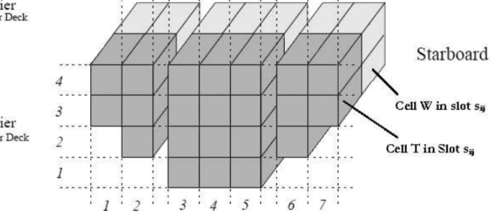
the stern to the bow. Containers are placed within each bay of a vessel according to a plan, referred to as the stowage plan. The containers are placed either below deck or above deck that is, inside the vessel or out in the open respectively. For later retrieval it is necessary to determine the exact location of a container. Several schemes exists in order to establish the position of each stowed container. The scheme, this report will use, is based on dividing the bays into slots fitting either one 40-foot container or two 20-foot containers. The slots within a bay is structured as a matrix, where each column is referred to as a stack and each row is referred to as a tier. Due to the shape of the vessel, some of the slots in the matrix are not allowed to hold any containers. Tiers are counted from the bottom of the matrix and up and stacks are counted from left to right. In order to identify two 20-foot container in a slot, a slot is further divided into two cells. As a consequence of stacking 20-foot container the term cell stack is introduced as cells in either one side of the stack or the other side of the stack.
Figure 3.2: An overview of the cell layout of a bay below deck.
Different height of containers may cause the actual location of the container to not match the positioning system. However in order to ease identification of neighboring slots, this report will regard the neighboring slots as the slots, which are immediately adjacent to it according to the positioning system.
Figure 3.3: Models the positioning system for two neighbor stacks. The stack to the left has been filled with standard containers, while the stack to the right have been filled with high cube containers. The dotted lines represent the actual position of each container according to the positioning system.
Containers stowed above deck and below deck are physically separated by hatches on the deck of the ship. In order to sail safely, a number of safety precautions are given as rules for stowage of containers. As these rules vary from above and below deck, this report will focus only on containers stored below deck. The safety requirements are described in the following:
Due to the physical shape of the ship, a height and a weight restriction is put on the contain-ers stowed in each stack. A maximum allowed height ensures that the containcontain-ers stowed
below deck fits below the hatches on the deck. The maximum allowed weight of a stack en-sures that the stress put on the hull of the ship by the stowed containers is within acceptable limits.
As the vessels travels overseas, the movement of the containers must be restricted. This is ensured by locking mechanisms attached to each corner of a container. Locking the containers in this manner restricts the placement of 20-foot containers such that they cannot be stowed on top of a 40-foot container.
Besides the physical properties of containers, goods have properties, which affect how con-tainers can be arranged. Other properties, which will affect the arrangement of concon-tainers are the IMO level of a container and temperature requirements.
In order to be able to reduce damages from accidents, containers with hazardous goods such as fireworks, needs to be placed at a safe distance from other containers with hazardous goods. The IMO level is a description of how close container with certain goods can be placed next to each other. This mechanism simplifies the requirements for specialized knowledge of handling hazardous goods.
Perishable goods such as fruit or meat needs to remain at a consistent and low temperature in order to avoid decomposition. Therefore these types of goods will need to be placed in containers with temperature controlling devices. Containers of this kind are referred to as reefers. Power is necessary to make the temperature controlling device running, and there-fore container can only be placed at designated areas with power supplying capabilities. Given that containers may be placed according to the requirements above, many different stowage plans may still be possible. Selecting one of them is arbitrary if no preference has been defined. However, each valid stowage plan posses different qualities and may be preferred depending on defined objectives. One of the objectives usually defined by any company is profit maximization. For container transportation this can in principle be achieved either by increase the fee on transportation or reducing the cost of transporting containers. Due to the competition increasing the fee is not always a viable solution. Con-sequently companies are forced to look at the cost instead. The objectives for reducing the cost are defined as objectives for the storage area stowage problem and are mainly centered around arranging containers. The objectives are to minimize the following: Overstows, usage of stacks, wasted space and usage of reefer slots.
Cranes are necessary to unload or load containers and the cost of loading or unloading a container is calculated by a fee. An objective follows that containers, which are to be unloaded in the current port, is to be placed on top of each stack in order to avoid unnec-essary container movement. Containers destined for future ports that are stacked on top of containers which are to be unloaded at the current port, is referred to as overstow contain-ers. An overstow is inferred for each container stacked on top of another container with a smaller discharge port number.
As more containers are stowed within the same bay at future ports, it is of interest to keep as many stacks within a bay empty as possible. This will in turn provide freedom when stacking future containers to maximize optimization criteria.
The stowage of containers needs to be as compact as possible in order to transport as many containers as possible. If an arrangement of containers are placed, such that there is some space, which cannot be replaced by a container then that space is considered wasted. Reefers can only be placed in designated areas, where power is being supplied. Placing non-reefer container in reefer slots may prevent a reefer container to be loaded onboard for some future port. Consequently as few reefer slots should be used to place non-reefer containers.
This section ends with a summary of the requirements for Storage Area Stowage Problem:
Physical requirements
Gravitation Each container has to be supported either by the bottom of the deck or by containers.
Max Height The total cellstack height cannot exceed the maximum cellstack height.
Max Weight The total weight cannot exceed the maximum weight.
No 20-foot On Top No 20-foot container can be on top of a 40-foot container.
Safety requirements
IMO Each container are assigned an IMO level, and the rules is that two IMO-2 container have to be separated by a stack with no IMO-2.
Each IMO-1 container cannot be adjacent to other container which is either IMO-1 or IMO-2.
Support requirements
Objectives
Overstow Each overstow will be penalized. Empty Stack Each empty stack will be rewarded. Wasted Space The amount of wasted space is penalized.
Reefer slot Each reefer slot which is occupied by a non-reefer container is penalized.
3.2
Formal definition of SASP
In the following, the requirements specified in the problem definition are translated into a formal definition of Storage Area Stowage Problem.
A slot is defined as the 40-foot stowage unit of a container vessel, uniquely identified by its bay, tier and stack position.
A stack denotes the slots of the same bay that have the same stack position. In each bay, stacks are counted from larboard to starboard, starting with 1.
Stack related notationsα= (sc, tcj, hj, wj)
sc : number of stacks
tcj ∈IN : number of tiers of stackj
hj ∈IR+ : height limit in foot of stackj
wj ∈IR+ : weight limit in kg of stackj
J ={1, . . . , sc} : indexed set of stacks
A storage area denote lower-deck slots having belonging to the same bay. Consequently, each slot of a storage area is uniquely identified by its 2-dimensional position consisting of the tier positionicounted bottom-up and its stack positionj counted from left to right. Since a slot may hold two 20-foot containers it is necessary to distinguish their positioning relative to the slot itself. A cell is defined as the part of a slot needed for a 20-foot container. The sides of a slot having place for two containers are referred to as the bow-side cell and the stern-side cell respectively. A slot, which can accommodate a single 20-foot container, is either placed on the bow-side or the stern-side depending on the ships physical structure.
W denotes the bow-side of a cell. T denotes the stern-side of a cell. Let Ldenote set of cells possible for a slot.
Slot related notationsβ ={S, ri,j, t20i,j, t40i,j, Li,j}
si,j : slot at stackjand tieri
ri,j ∈IB : trueifsi,j is a reefer
t20
i,j ∈IB : trueifsi,j can hold 20-foot containers
t40
i,j ∈IB : trueifsi,j can hold 40-foot containers
L={W, T} : set of sides of a slot
Li,j ⊆L : set of cells that can be taken by 20-foot
containers ift20
i,j istrueor by 40-foot
containers ift40
i,j istrue
S ={si,j : 1≤j ≤sc∧1≤i≤tcj} : indexed set of slots
C0is the set of containers already on board before arriving to port1, and remain on board after the vessel leaves port1.
C1is the set of containers to be loaded into the storage area at port1.
Cdenotes the entire set of containers, which will be onboard the ship when departing from port1i.e. C =C0 ∪ C1.
P is the number of ports on the route the vessel sails.
Properties of containerc∈C
dpc ∈ {1, . . . , P} : discharge port number of containerc
wc ∈IR+ : weight in kg of containerc
hc ∈ {8.5,9.5} : height in feet of containerc
imoc ∈ {0,1,2} : IMO-level of containerc
lc ∈ {20,40} : length in feet of containerc
rc ∈IB : trueif containercis a reefer
Besides the properties defined above, on board containers specify their load port and their stowage position in the vessel.
Additional properties of a containerc∈C0
lpc ∈ {1, . . . , P} : load port number of containerc
pc ∈S×2L : on board position of containerc
For convenience,γdenotes the collection of container related properties:
An assignment or a stowage plan is an arrangement of containers within the vessel.
A0 :C0 →S×2Ldefined byA0(c) =p
c is the stowage plan for containers on board.
A1 :C1 →S×2Lis the stowage plan for containers to be loaded at port1.
Definition 3.1 (Assignment) An assignment of containers inCis a total functionA:C →
S×2L
A(c) =
A0(c) ifc∈C0
A1(c) ifc∈C1
The projections on slot and cell for a containercare:
AS :C→Sis the projection ofAonS.
AL :C →2Lis the projection ofAon2L.
Definition 3.2 (Storage Area Stowage Problem(SASP)) The storage area stowage prob-lem is a 5-tuple(C0, C1, α, β, γ).
Example 3.1 Consider the stowage area shown in Figure 3.7, consisting of a single stack
and a container on board.
c0
Figure 3.4: Stowage area with one stack.
Stack properties areα= (sc= 1, tc1 = 5, h1 = 43, w1 = 14000) The set of slots isS ={s1,1, s1,2, s1,3, s1,4, s1,5}
Slot properties are:
β t20
i,j t40i,j Li,j ri,j
s1,5 true false {W} false
s1,4 true true {W, T} false
s1,3 true true {W, T} true
s1,2 true false {W, T} true
s1,1 true false {W, T} true
The set of containers on board is: C0 ={c0} The set of containers to be loaded is:C1 ={c
Container properties are: γ dpci lci rci lpci pci wci hci imoci c0 2 20 true 0 (s1,1, W) 14000 8.5 0 c1 2 20 true - - 1400 8.5 0 c2 3 40 false - - 2800 8.5 0 c3 4 20 true - - 1400 8.5 0 c4 2 20 false - - 1400 8.5 0 The assignment for containers on board isA0(c
0) =pc0 The SASP of this configuration is(C0, C1, α, β, γ, A0)
Before enumerating the constraints and objectives of the problem, some additional sets are constructed, that will ease the writing.
Container sets
Cz={c∈C : lc =z} : containers of lengthz ∈ {20,40}
CIMO-z={c∈C : imoc =z} : containers having IMO levelz ∈ {0,1,2}
Cj ={c∈C : ∃i .1≤i≤tcj∧AS(c) =si,j} : containers assigned to stackj
Cl
j ={c∈C : c∈Cj ∧l ∈AL(c)} : containers assigned to sidelof stackj
Ci,j ={c∈C : AS(c) =si,j} : containers assigned tosi,j
Cnr ={c∈C : ¬rc} : non reefer containers
Slot and Cell Sets
SIMO-1
i,j ={si−1,j, si+1,j, si,j−1, si,j+1} : slots that cannot stow an IMO-1 container in case slotsi,j holds an IMO-1 container
SIMO-2
i,j ={sk,j−1 : 1≤k ≤tcj−1} ∪ : slots that cannot stow an IMO-2 container
{sk,j+1 : 1≤k≤ tcj+1} ∪ in case slotsi,j holds an IMO-2 container
{sk,j : 1≤k≤i ∨ i < k ≤tcj}
Snr ={A(c) :c∈C
nr} : cells storing non-reefer containers
Cell coverage
Ti,j =
S
c∈Ci,jAL(c) : cells covered by containers assigned tosi,j
oi,j ⇔Li,j =Ti,j : oi,j true if slotsi,j is fully occupied
oW
i,j ⇔W ∈Ti,j : oWi,j true if the bow side of slotsi,j is occupied
oT
i,j ⇔T ∈ Ti,j : oTi,j true if the stern side of slotsi,jis occupied
Constraints
CT1 All containers are assigned to a cell of a slot
∀c∈C . AS(c) =si,j ⇒AL(c)⊆Li,j CT2 A cell can hold at most 1 container
∀c, c′ ∈C . c 6=c′ ∧AS(c) = AS(c
′
)⇒AL(c) ∩ AL(c
′
) = ∅
CT3 A 40-foot container must cover both sides of a slot
∀c∈C40.|AL(c)|= 2
CT4 A 20-foot container is allowed to cover one cell in a slot
∀c∈C20.|AL(c)|= 1
CT5 Assigned slots above tier 1 must form stacks (gravity constraint)
∀si,j ∈S . oi,j∧j >1⇒oi−1,j
∀si,j ∈S . oTi,j∧j >1⇒oTi−1,j
∀si,j ∈S . oWi,j∧j >1⇒oWi−1,j
CT6 20-foot containers cannot be stacked on top of any 40-foot container
∀c40 ∈C40∀c20 ∈C20. AS(c40) =si,j ⇒AS(c20)6=si+1,j CT7 The height of each cell stack is within its limits
∀j ∈J∀l ∈L . P
c∈Cl
jhc ≤hj
CT8 The weight of each stack is within its limits
∀j ∈J . P
c∈Cjwc ≤ wj
CT9 Reefer containers must be placed in reefer slots
∀c∈C . rc∧AS(c) =si,j ⇒ri,j
CT10 IMO rules are satsified for each container
∀c∈CIMO-1 ∪ CIMO-2∀c ′ ∈CIMO-1. AS(c) =si,j ⇒AS(c ′ )∈/ SIMO-1 i,j ∀c, c′ ∈CIMO-2. AS(c) =si,j ⇒AS(c ′ )∈/ SIMO-2 i,j
Objectives
OE1 Minimize overstows
There is a cost penalty of one unit for each container in a stack overstowing another container below it in the stack. The unit weight isWov.
There is an overstow between any two distinct containers in case they belong to the same cellstack and the discharge port of the container stowed at the lower tier is higher than the discharge port of the container stowed at the higher tier.
The binary relation≺onS ×S defines whether two slots belong to the same stack and whether the first slot is located below the second slot:
si,j ≺si′,j′ ⇔i < i′ ∧ j =j′
ov:C×C →IBdefines if there is an overstow between two containers:
ov(c, c′)⇔c6=c′ ∧dpc < dpc′ ∧AS(c)≺AS(c
′
)∧AL(c) ∩ AL(c
′
)6=∅
Definition 3.3 (Overstow cost) Fov(A) =
{(c, c
′
)∈C×C : ov(c, c′)}
OE2 Minimize the space wasted in a stack
The cost penalty is the length of wasted space. The unit weight isWws.
A stack consists of two cellstacks that do not necessarily have the same number of containers stacked into them. Therefore the two cellstacks can grow to different heights. The wasted space of the stack is defined as the sum of the wasted space of its two cellstacks. There is no wasted space in a cellstack, if there is enough space space to fit a standard container, otherwise the wasted space is the space left in the cellstack.
fs:J ×L→IRdefines the available space on sidelof stackj:
fs(j, l) =hj−
X
c∈Cl j
hc
ws:J×L→IRdefines the wasted space on sidelof stackj:
ws(j, l) =
0 iffs(j, l)≥hst
fs(j, l) iffs(j, l)< hst Definition 3.4 (Wasted space cost) Fws(A) =
P
Figure 3.5: Skewed positioning system
Due to a skewed positioning of containers in the right stack, wasted space is introduced in the top in which no containers can be placed.
OE3 Avoid loading non-reefers into reefer slots
The cost penalty is one unit for each non-reefer container in a reefer slot. The unit weight isWr.
Definition 3.5 (Reefer cost) Fr(A) =
{(si,j, l)∈Snr : ri,j}
OE4 Avoid starting new stacks
The cost penalty is one unit per new stack used. The unit weight isWes. Definition 3.6 (Empty stack cost) Fes(A) =
{j ∈J : |Cj|>0}
Definition 3.7 (Cost of an assignment) The cost of a solution is the weighted sum of the costs defined for objectives (OE1) - (OE4):
F(A) = WovFov(A) +WwsFws(A) +WrFr(A) +WesFes(A)
Definition 3.8 (Valid Solution of the SASP) A valid solution of SASP is an assignment of containers to be loaded in port 1A1 : C1 → S×2L, such that the total assignment of containersA:C →S×2Lsatisfies constraints (CT1)-(CT10).
Definition 3.9 (Solution space) The solution space for SASP is the setA1 of all valid
solutions.
Definition 3.10 (Optimal Solution of the SASP) An optimal solution A1∗ of SASP is a
valid solutionA1′ that minimizes the cost functionF(A).
A1∗ = argmin
A1′∈A1
F(A)
Example 3.3 Consider SASP defined in Example 3.1:
A1(c 1) = s1,1,{W} A1(c 2) = s1,3,{W, T} c2 A1(c 3) = s1,2,{T} c3 c4 A1(c 4) = s1,2,{W} c0 c1 Figure 3.6:A valid solution with cost1150.
A1(c 1) = s1,2,{W} A1(c 2) = s1,3,{W, T} c2 A1(c 3) = s1,1,{T} c1 c4 A1(c 4) = s1,2,{T} c0 c3 Figure 3.7:An optimal solution with cost950.
Chapter 4
Evaluating CSP representations of SASP
Many variations exist on how to represent the Storage Area Stowage Problem as a con-straint satisfaction problem. Three possibilities have been considered on how to model SASP as a CSP - namely ”Container as variables and slot as domain values”, ”Slot as
variables and container as domain values” and ”Cell as variables and container halves as domain values”. These suggestions will be referred to as container-model, slot-model
and cell-model respectively. A presentation for each model is given with a brief descrip-tion, followed by how domain values are pruned then pros and cons are outlined. After the presentation, a scoreboard follows with a conclusion of which model was chosen. In this chapter the initial step of how to translate the constraints into propagators is shown by identifying the pruning operations.
4.1
Pruning operations
Before outlining each model, the pruning operations, which are required to satisfy the con-straints in SASP, are presented. The necessary pruning operations have been identified by analyzing each constraint and extracting the operations required. Table 4.1 shows the pruning operations identified. Table 4.2 illustrates, how each constraint is covered by some pruning operations. As the table shows, no pruning could be inferred from CT1, so this constraint must be implemented by other means.
PG1 - Uniqueness
Each container to be loaded are used from the same pool, which implies placed containers cannot be considered for another slot. Each cell can only be used once.
PG2 - Gravity
When placing a container sufficiently high in a stack, it is required that some containers are placed underneath it, in order to avoid it from falling to the bottom of the ship. The term support is introduced to state that a container is required in order to ensure that a placed
ID Name Constraint Pruning
PG1 Uniqueness CT1 N/A
PG2 Gravity CT2 PG1
PG3 Reefer CT3 PG8
PG4 Pick IMO-1 container CT4 PG1
PG5 Pick IMO-2 container CT5 PG2
PG6 Pick 20-foot container CT6 PG6, PG7
PG7 Pick 40-foot container CT7 PG9
PG8 Cover 40-foot container CT8 PG10
PG9 Height CT9 PG3
PG10 Weight CT10 PG4, PG5
Table 4.1: Pruning operations Table 4.2: Pruning coverage
container stays at its position.
PG3 - Reefer
A reefer container cannot be in a non-reefer slot. However, since it is given by the problem which slots have reefer capability this pruning can occur prior to the search.
PG4 - Pick IMO-1 container
According to the IMO constraint, neighboring slots is not allowed to accommodate IMO-1 container once an IMO-1 have been placed in a given slot.
PG5 - Pick IMO-2 container
According to the IMO constraint, slots in the current and neighboring stacks is not allowed to accommodate IMO-2 containers, once a given slot in a current stack is assigned with an IMO-2 container. Furthermore, neighboring slots to the given slot may not contain an IMO-1 container as well.
PG6- Pick 20-foot container
It should not be possible to place any 20-foot container on top of a 40-foot container. Therefore in the case when a 20-foot container has been placed no 40-foot container can be considered for any slots below it.
PG7 - Pick 40-foot container
A constraint states that it should not be possible to place any 20-foot container on top of a 40-foot container. Therefore, in the case where a 40-foot container has been placed, no 20-foot container can be considered for any slots above it.
PG8 - Cover 40-foot container
A 40-foot container must cover an entire slot.
PG9 - Height
In the problem definition, a height limitation constraint has been given. Since all stacks are divided into slots and only two different container heights available, pruning will not
occur until one empty slot in a given stack remains. For this reason, no pruning will occur based on the height constraint. An alternative mechanism needs to ensure that the height limitation is respected.
PG10 - Weight
The weight constraint states that each stack cannot exceed its weight limit wj. The
re-maining weight, is the weight that can be added to stackj, before exceedingwj no matter
if some containers have been placed or not. The remaining number of slots, will be the number of slots, where nothing has been placed yet and the remaining available containers are the containers, which still needs to be placed within the bay. In the general case it will be that either all remaining available containers can be placed within stack j or some n
lightest containers can be placed before exceeding the remaining weight. Ifnis less than the number remaining empty slots, then it can be inferred that onlynslots can be filled up with thenlightest containers before exceeding the weight limitation. Therefore the rest of the slots cannot be assigned to any container. Since gravity rule requires that containers are supported, the bottom available slots have to be filled and the upper available slots can be left with nothing.
4.2
Container-model
Variables: ContainerDomain values: Slot
Approach: The idea behind this model is to have containers represented as variables and
then consider, which slot each container should be assigned to. Since this is the task of SASP this representation seems to be a natural choice for representing the CSP-model.
Pruning:
PG1 Slot si,j can be pruned away as a candidate value, when it has been fully covered
by containers. When the assigned container covering the slot is a 40-foot container,
si,j can be removed immediately. Assigning a 20-foot container, requires thatsi,j is
checked for whether it has been fully covered before being pruned away.
PG2 When placing containers it has to be ensured that there are enough containers to
support it. When the number of containers needed to support some other container is the same as the number of available containers to be placed, then slots, which do not have any placed containers above the picked slot, can be pruned away as candidate values from all the available containers to be placed.
PG3 Each reefer container can only be placed in a reefer slot, while a non-reefer container
PG4 Picking some slotsi,j for an IMO-1 container prunes any slot according to the IMO
constraint for any IMO-1 container.
PG5 Picking some slotsi,j for an IMO-2 container prunes any slot according to the IMO
constraint for any IMO-1 and IMO-2 container.
PG6 Picking some slotsi,j for a 20-foot container prunes any slot in stackj below tieri
as candidate values for any 40-foot containers.
PG7 Picking some slotsi,j for a 40-foot container prunes any slot in stackj above tier i
as candidate values for any 20-foot containers.
PG8 40-foot container has the same dimension as a slot, it is therefore ensured by the
model that a 40-foot container fully covers a slot.
PG9 As described previously this pruning operation will not be considered.
PG10 When only the n lightest containers can fit in a stack j. All available containers, which are not among the n lightest containers needs to get slots pruned away. The slots, which are required to be pruned away, are those described in PG10 in section 4.1.
Advantages:
• Since the search goes through all containers, it is ensured by the model that every container will be assigned.
• Reefers can be pruned prior to search • Do not need to prune anything for PG8.
Disadvantages:
• The gravity constraint is difficult to ensure, since this model relies on forcing some containers to pick specific cells.
• Placed container may potentially affect where all other containers can be placed. For instance placing an IMO-1 container will affect where all other IMO-1 containers can be placed.
• The number of variables, which will be affected by PG10 are all unassigned vari-ables.
The following model takes the reverse of the previous approach by looking at the stowage area and examines what can be fitted into each slot. Since there cannot be more contain-ers than slots available, some slots are assigned but left empty. An air value has been introduced to denote that a slot remains empty.
4.3
Slot-model
Variables: SlotDomain values: Containers
Approach: This model uses the slots as variables and containers as domain values. In
example, for each slot, one can chose which container it should accommodate. Since a slot can accommodate a 40-foot container and some containers may be 20-foot long, placing two 20-foot containers within a slot poses an issue. One approach is to construct pairs of 20-foot containers, which will result in|C20|2 of such combinations. In addition, one 20-foot containers may be placed in a slot alone, leaving half of the slot empty. Furthermore, special slots exists, which can only hold a single 20-foot container.
Pruning:
PG1 When a container chas been used, it needs to be pruned away as a possibility from all other unassigned slots. Ifcis a 20-foot container, then all domain values, in which
cappears, has to be pruned away as a candidate value as well.
PG2 When a container is placed in a slot, all slots underneath it cannot select the
intro-duced air value for assignment. That is, when a 40-foot container is placed in slot
si,j, the air value is pruned away from the domain of any variable positioned in the
same stack beneathsi,j.
PG3 Each reefer container can only be placed in a reefer slot, while any non-reefer
con-tainer can be placed in either a reefer or a non-reefer cell.
PG4 Picking some IMO-1 container for slotsi,j prunes any IMO-1 container as candidate
value for slots according to the IMO constraint.
PG5 Picking some IMO-2 container for slotsi,j prunes any IMO-1 and IMO-2 containers
as possible candidate values according to the IMO constraint.
PG6 Picking some 20-foot container for slotsi,jprunes any 40-foot container as candidate
value for slots in stackj below tieri.
PG7 Picking some 40-foot container for slotsi,j prunes any 20-foot containers as
candi-date value for slots in stackjabove tieri.
PG8 40-foot container has the same dimension as a slot, it is therefore ensured by the
model that a 40-foot container fully covers a slot.
PG10 Each stackj will only be able to accommodate then lightest containers before ex-ceeding the weight limitation. All other containers to be placed can be pruned away as candidate values from any slots inj. Furthermore if the number of slots available in the stack exceeds n it can be inferred that all but the lowestn slots will have to accommodate air, since any containers above tier 1 needs to be supported.
Advantages:
• The search can be done such that the slots are filled in a bottom up approach, thereby respecting the gravity constraint.
• Reefers can be pruned prior to search.
• Simple to reason about containers placed in a stack. • Do not need to prune anything for PG8.
• The number of variables, which will be affected by PG10, are limited to only one stack when using this model, as opposed to the container-model, where all variables are affected.
Disadvantages:
• Since any slot initially can pick air as a candidate value, not all containers may be placed within the stowage area. This has to be ensured by introducing additional propagator.
• Implacable IMO-1/IMO-2 containers are potentially discovered late.
4.4
Cell-model
Variables: CellsDomain values: Containers
Approach: The drawback of using the slot-model, is the number of domain values. To
address this issue, the following model is introduced, which avoids the combination of 20-foot containers by using cells as variables. By having cells as variables one can fit exactly a 20-foot container. However, 40-foot containers will not fit within a cell. This issue can be handled by splitting 40-foot containers into matching halves. For convenience, when a container half is mentioned in this section, it refers to both a 20-foot container or a 40-foot half container.
PG1 Picking containercfor slotsi,j prunescfrom any other slot.
PG2 When a container is placed in a cell, all cells underneath it can not select the
intro-duced air value for assignment. That is, when a 40-foot container is placed in slot
si,j, the air value is pruned away from the domain of any variable positioned in the
same stack beneathsi,j.
PG3 Each reefer container can only be placed in a reefer cell, while a non-reefer container
can be placed in either a reefer or a non-reefer cell.
PG4 Picking some IMO-1 container celllin slotsi,jprunes any IMO-1 container in slots
according to the IMO constraint.
PG5 Picking some IMO-2 container celll in slotsi,j prunes any IMO-1 and IMO-2
con-tainer in slots according to the IMO constraint.
PG6 Picking some 20-foot container for celllin slotsi,jprunes away any 40-foot
contain-ers in cells below tieriin stackj and on the same side as celll.
PG7 Picking some 40-foot container for celllin slotsi,jprunes away any 20-foot
contain-ers in cells below tieriin stackj and on the same side as celll.
PG8 40-foot container needs to be cut in half to fit a cell, therefore ensuring that the two
halves are placed next to each other is required. This can be achieved by pruning all domain values except the other half from the domain of the neighbor cell.
PG9 As described previously this pruning will not be considered.
PG10 Each stackj will only be able to accommodate then lightest containers before ex-ceeding the weight limitation. The containers to be placed, can be pruned away as candidate values from any cells inj, which only can accommodate air.
Advantages:
• The search can be done such that each stack is filled bottom up, thereby respecting the gravity constraint in a natural way.
• Maintaining 20-foot container pairs is not needed, which results in a narrower search tree than the slot-model, due to smaller domains.
• Non-reefer cells can have their initial domains pruned to only select the non-reefer container halves.
• The number of variables, which will be affected by PG10, are limited to only one stack when using this model, as opposed to the container-model, where all variables are affected.
• Simple to reason about containers placed in a stack. • Do not need to prune anything for PG8.
Disadvantages:
• Number of variable is doubled, compared to the slot-model, which results in a deeper search tree.
• Additional constraints needs to be added:
– 40-foot container half has to be placed next to its other half.
– 20-foot containers cannot be placed next to 40-foot container halves.
4.5
Conclusion
The variable and domain sizes are summarized in table 4.3. Assuming that there are suffi-cient slots for the containers, the table shows that the cell-model has the most variables and thus results in the deepest search tree. The container-model will have the lowest number of variables and therefore have the shallowest search tree. The domain sizes shows that slot-model has the largest domain size and therefore also provides the widest search tree. The cell-model result in the narrowest search tree due to the domain size.
Container-model Slot-model Cell-model
Variables |C| |S| |S||L|
Domains |S| |C40|+|C20|2+ 2|C20| |C| Table 4.3: space complexities for the given elements in the future application
Table 4.4 shows how many variables are affected when pruning based on a constraint is carried out. Let tc = maxj∈{1,...,sc}{tcj} denote the number of tiers for the stack in the
bay, which has the most tiers. As the table shows, the container-model will depend on the number of containers when pruning. For the other two models the amount of pruning is mainly dependent on the stack size. Since it is expected that the number of slots which appears in a stack is significantly less than the number of containers, it is expected that either the slot-model or the cell-model is affecting less variables than the container-model. The number of domain values in the slot-model is significantly higher than in the cell-model. Based on the above observation, the model chosen is the cell-cell-model.
Container-model Slot-model Cell-model
PG1 - Uniqueness |C| |S| |S||L|
PG2 - Gravity |C| |tc| |tc|
PG3 - Reefer - -
-PG4 - Pick IMO-1 container |C| 4 9
PG5 - Pick IMO-2 container |C| 3|tc| 3|L||tc|
PG6 - Pick 20-foot container |C| |tc| |L||tc|
PG7 - Pick 40-foot container |C| |tc| |L||tc|
PG8 - Cover 40-foot container - - 1
PG9 - Height - -
-PG10 - Weight |C| |tc| |tc|
Table 4.4: Shows the maximum number of affected variables when performing dif-ferent pruning operations in the three difdif-ferent models.
Chapter 5
CSP representation of SASP
Based on the analysis for selecting a proper representation of SASP, the CSP-Model needs to be detailed further. This chapter presents the CSP-Model in terms of variables, domains and propagators. It is shown how pruning operations can be transformed into propagators.
5.1
Variables
Each variable in the CSP model corresponds to a cell as defined in the SASP. The set of variables is:
X ={xli,j : si,j ∈S∧l∈Li,j}
Table 5.1: Model specific variable sets
XIMO-z
i,j ={xli,j ∈X : si,j ∈Si,jIMO-z} : variables that cannot stow an IMO levelz,
when an IMO levelzhas been placed insi,j
XR={xl
i,j ∈X\ S : ⊥∈ D/ (xli,j)} : all unassigned variables, which cannot
accommodate air
For convenience, a neighboring operation is defined on the set of cells L, to denote the other side of a cell within a slot:
W =T, T =W.
5.2
Domains
Since variables are cells, a variable cannot be assigned to a 40-foot container. Consequently, 40-foot containers are divided into two halves, each half maintaining the properties of the
original 40-foot container. To identify the two halves that make up an original 40-foot con-tainer, the halves are given the same unique identifier. In this model, the container term is used both for 20-foot containers and 40-foot container halves. A 40-foot container half is marked similarly to a cell, as being bow or stern.
Model specific container sets
CH
40={cT, cW : c∈C40} : 40-foot container halves
CH
nr ={cλ ∈C40H, c ∈C20 : ¬rc} : non-reefer 40-foot halves and 20-foot containers
CH
r ={cλ ∈C40H, c ∈C20 : rc} : reefer 40-foot halves and 20-foot containers
CH
IMO-z ={c
λ ∈CH
40, c∈C20 : imoc =z} : 40-foot halves and 20-foot containers with IMO-z
The neighboring operation on the set of cells still holds. That is, the corresponding half of a 40-foot halfcλiscλ.
In case the bay has more cells than containers, some of the cells will remain empty. Let⊥ denote the domain value that indicates that a cell is left empty. The ”air” term is used as a synonym for⊥. The properties for⊥are:
h⊥ = 0, w⊥ = 0, l⊥= 0, imo⊥ = 0, r⊥ =false, lp⊥= 0anddp⊥= 0.
The domain of a variable consists of the containers the cell can accommodate. Some slots can stow a single 20-foot container. Therefore 40-foot containers are excluded from the do-main of the cells belonging to these slots. Reefer containers can only be placed into reefer slots and therefore reefer containers are excluded from the domain of non-reefer cells.
LetD(xl
i,j)be the initial domain for each variablexli,j.
D(xl i,j) = CH
40 ∪ {⊥} : ¬t20i,j ∧t40i,j ∧ri,j
(CH
40 ∩ CnrH) ∪ {⊥} : ¬t20i,j ∧t40i,j ∧ ¬ri,j
C20 ∪ {⊥} : t20i,j ∧ ¬t40i,j ∧ri,j
(C20 ∩ CnrH) ∪ {⊥} : t20i,j ∧ ¬t40i,j ∧ ¬ri,j
CH
40 ∪ C20 ∪ {⊥} : t20i,j ∧t40i,j ∧ri,j
((CH
40 ∪ C20) ∩ CnrH) ∪ {⊥} : t20i,j ∧t40i,j ∧ ¬ri,j
{c} : ∃c∈C20. A0S(c) = si,j∧l ∈A0L(c)
{cλ} : l =λ∧ ∃cλ ∈CH
40. A0S(c) =si,j ∧l∈A0L(c)
∅ : ¬t20
i,j ∧ ¬t40i,j Example 5.1 Consider the SASP defined in Example 3.1.
The set of variables is:
X ={xW1,1, x T 1,1, x W 1,2, x T 1,2, x W 1,3, x T 1,3, x W 1,4, x T 1,4, x W 1,5}
The set of 20-foot containers is:
C20={c0, c1, c3, c4} The set of 40-foot container halves is:
CH
40 ={cW2 , cT2} The initial domains are :
D(xW 1,1) ={c0} D(xT 1,1) ={c1, c3, c4,⊥} D(xW 1,2) ={c1, c3, c4,⊥} D(xT 1,2) ={c1, c3, c4,⊥} D(xW 1,3) ={c1, c2W, cT2, c3, c4,⊥} D(xT 1,3) ={c1, c2W, cT2, c3, c4,⊥} D(xW 1,4) ={cW2 , cT2, c4,⊥} D(xT 1,5) ={c4,⊥}
5.3
Additional constraints and pruning operations
Besides the constraints given in SASP, this model introduces three additional constraints:
CT11 The two halves of a 40-foot container must be placed in the same slot
∀c∈C40. xli,j =c λ ⇒
xli,j =c λ
CT12 A cell that accommodates a 20-foot container excludes the possibility of its neighbor
cell to accommodate a 40-foot half
∀xli,j, x l i,j ∈X . x l i,j =c∧c∈C20∧xli,j =c′ ⇒c′ ∈/ C H 40
CT13 Allowing each container only to appear once
∀xl i,j, x l i,j ∈X . x l i,j 6=x l i,j ∧x l i,j =c∧x l i,j =c′ ⇒c6=c′
![Figure 3.1: An overview of the layout of a ship. [7]](https://thumb-us.123doks.com/thumbv2/123dok_us/1406793.2688322/20.918.124.812.55.275/figure-overview-layout-ship.webp)