A Reality-Based Method for Valuing Stocks

(1)

Current Draft September 3, 2001

A Reality-Based Method for Valuing Stocks

Scott A. Hoover†

Washington and Lee University

Frederic P. Sterbenz

University of Wyoming and University of Wisconsin-Madison

†_{The first author may be contacted at Department of Management; Washington and Lee University; Lexington, VA} 24450; phone: 540-463-8178; email: [email protected]. The second author may be contacted at University of Wisconsin-Madison; School of Business; Finance Department; 975 University Avenue; Madison, WI 53706; phone: 608-263-2649; email: [email protected] or [email protected]. We thank John Wachowicz, Jr. for useful comments.

(2)

A Reality-Based Method for Valuing Stocks

Abstract: We present a model that uses analyst earnings growth estimates and price-to-earnings ratios to project the expected cash flows to shareholders. Those cash flows can then be discounted to estimate the fundamental value of stocks. Our model specifically addresses growth estimates that cover finite periods of time. The primary use of our model is in comparing stocks in the same industry, but the model might also be used for industry selection or market timing. We also examine the implications for using the PEG ratio to identify potentially mispriced stocks.

(3)

Introduction

In many disciplines, instructors in introductory courses face the problem of teaching theory that cannot easily be applied in the real world. Students often ask why they need to know the material if it will not be useful in their career. The answer, which is seldom satisfactory to students, is often that the intuition is important. This scenario happens often in finance when instructors teach the Gordon model of stock valuation, which Bodie and Merton (2000) refer to as the Discounted Dividend Model. Nearly all introductory finance textbooks present this model,1 yet interested students quickly discover that the model falls apart when dividend growth rates are high, leading to very large or even negative estimates of stock value. To correct this problem, some use a growth phase model in which dividends grow at a high rate initially, but then drop to a reasonable long-term rate. Such a model is suitable if that long-term rate can be accurately estimated. A second problem is one that plagues both the Gordon model and the growth phase extension.2 When firms do not pay dividends, those models imply that the stock is worthless. The implication is that the models provide basic intuition, but are not very useful in practice.

Our goal then is to provide a variation of the Gordon model that retains the important intuition of Gordon yet is readily applicable in real world situations. We have taught this methodology in the classroom for several years with great success. Students are genuinely excited to learn an approach that can be used in their everyday investment lives. Furthermore, the approach allows instructors to carefully and analytically establish the relationship between dividends, earnings, earnings growth estimates, price-to-earnings (P/E) ratios, and stock value.

Our model is closely related to that of Malkiel (1963) and can be considered an extension of it. We arrive at the same valuation equation as Malkiel, but then demonstrate how to apply

(4)

the model given information currently available. The model is similar to Gordon’s in that it relies on the discounted value of expected cash flows to shareholders. The model differs, however, in that we do not assume an infinite series of cash flows. Rather, we value the stock as if it will be sold at some future date. We estimate the value of the stock at that date by examining current earnings and earnings growth estimates. In equilibrium, of course, the estimated value of the stock at that date will be the expected value of expected dividends from that date forward. In that way, we avoid the complication of estimating dividends forever.

It is natural to ask how a given earnings growth rate and a given earnings level relate to a stock price. We provide a reasonable method to value common stocks based on earnings growth rates. This is desirable because analysts produce estimates of growth in earnings rather than focusing on dividends. Typical valuation models can be applied in two ways. First, they can be used to determine whether a stock is a good buy relative to other stocks. Second, they can be used to determine whether a stock is a good buy relative to not buying it. Our technique seems better able to address the former. Furthermore, our technique is applicable with relatively short-term earnings growth estimates and is robust to small changes in those estimates. In contrast, the Gordon model (which requires a long stream of dividend estimates) often provides dramatic differences in stock value when growth rates change slightly. Furthermore, the Gordon model is difficult to apply when companies do not pay dividends. The typical approach is to assume that the company will eventually pay dividends and try to estimate what those dividends will look like. This is a daunting task that seldom leads to reasonable results.

Analysts typically provide earnings growth estimates for up to five years. These are collected and reported by I/B/E/S International, Inc. <www.ibes.com> and others, and are available on many web sites.3 Based on these growth rates, we can estimate earnings per share

(5)

five years from now. We then estimate share price in five years by multiplying by an appropriate P/E ratio. In determining this P/E ratio, we generally assume that all firms within a given industry have the same expected P/E ratio in five years. The justification for this is the mean reversion of earnings growth rates. Said differently, it is difficult to guess whether a given firm will be below, at, or above average within the industry five years from now. Our best estimate today is likely to be that the firm will be average. This does not imply that we assume that the firms will be identical in five years. Rather, we assume that firm P/E ratios follow a stochastic process in which similar firms have the same expected P/E ratio in five years. As Malkiel (1963) points out,4 using an extraordinary growth rate and using an extraordinary future P/E ratio would in effect overstate the impact of the extraordinary growth. Doing so is equivalent to assuming extraordinary growth well beyond five years. Of course there may be exceptional cases where a company is expected to have an atypical P/E ratio well into the future, but our approach is easily adjusted in those cases. We therefore use the same projected P/E ratio for similar firms, but discuss how the model might be adapted to handle exceptional firms.

The model has several significant advantages when comparing groups of similar stocks. First, the estimate of the expected P/E ratio in five years is not critically important. In fact, we generally arrive at the same rank orderings of stocks regardless of the P/E ratio chosen. The intuition is simple. If we underestimate the P/E ratio by, say, 50%, we underestimate it by 50% for all the stocks, thus reducing our estimate of stock values by a similar percentage. This typically does not change the outcome when we look at which stocks appear to be the most mispriced. The second advantage is that the estimate of the expected market return is not critically important. If we rely on the Capital Asset Pricing Model to determine discount rates (as most textbooks do), we are subject to potentially substantial errors due to the difficulty of

(6)

estimating the expected market return. The rule of thumb that the market risk premium (the expected market return less the risk-free rate) is 5%-9% allows for significant errors in discount rates and hence in estimates of stock value. Our technique is robust to changes in the expected market return because such changes tend to affect similar stocks by similar amounts. Thus, misestimating the expected market return does not typically alter the rank orderings of stocks.5

The point of our paper is not to recommend a method for use in picking stocks or practicing market timing. Rather, our goal is to present a common sense approach to stock valuation that allows us to draw rational conclusions about the relationship between dividends, earnings, and P/E ratios. An additional goal is to provide a method of valuation that uses data available on the internet. The usefulness of this method for picking stocks will depend in part on the accuracy and reliability of the analysts’ forecasts of earning growth.

Although we do not explicitly consider the idea in this paper, the methodology is not restricted to using P/E ratios. Price-to-sales or other ratios might also be used. This suggests that the model might be used to estimate the value of companies with zero dividends and negative earnings. The difficulty in those cases is the need to estimate the future growth of sales or other variables under consideration.

The remainder of the paper is organized as follows. Section I describes the basic model. Section II demonstrates the application of the model. In Section III, we comment on the relationship between leverage and P/E ratios. PEG Ratios are discussed in Section IV. The model is applied to the Pharmaceutical industry in Section V. Section VI concludes.

(7)

I. The Simple Model

Suppose that a company recently paid a dividend of D0 and has current earnings of E0.6

Earnings are expected to grow at a rate of g for the next T years. The company is expected to continue paying dividends with the same dividend payout ratio (D/E). An implication of the constant dividend payout ratio is that dividends are also expected to grow at the rate g. The required return on the company’s stock is r. We use the Capital Asset Pricing Model (CAPM) to determine r. The expected P/E ratio for the company’s stock at date t is . The market price of the stock today is S

t

Qˆ

0 and the true value of the stock at date t is Vt.

The value of the stock today should be the present value of the expected cash flows to shareholders. In other words, the value today should be the present value of all future dividends. Thus, (1)

₍

) (

1

)

... ˆ 1 ˆ 1 ˆ 3 3 2 2 1 0 + + + + + + = r D r D r D V . In general, (2)

(

)

(

)

(

1

)

... ˆ 1 ˆ 1 ˆ 3 3 2 2 1 1 ₊ + + + + + = + ₊ + + + + t t t t t t t r D r D r D V .

In reality, this equation is difficult to apply. Few analysts estimate earnings for more than five years into the future, which makes it difficult to estimate both earnings and dividends beyond that. Said differently, because g applies only to a finite period of time, we cannot estimate dividends for an infinite period of time. We can, however, value the stock by noting that (1) and (2) imply (3)

₍

) (

)

(

) (

)

T T T T r V r D r D r D V + + + + + + + + = 1 ˆ 1 ˆ ... 1 ˆ 1 ˆ 2 2 1 0

(8)

for any time T. Valuing a stock using (3) is equivalent to valuing the stock under the assumption that it will be sold in T years. This suggests that if we can reasonably estimate V , then we can avoid the problem of estimating an infinite number of dividends.

T

ˆ

T

Vˆ can be determined by estimating the company’s earnings at date T and multiplying them by the expected P/E ratio. The expected earnings are

(4) Eˆ_T = E₀

(

1+g

)

T and the expected stock value is7

(5) Vˆ_T = Eˆ_TQˆ_T = E₀

(

1+g

)

T Qˆ_T

The expected dividends can be projected as . This gives a general formula for valuing a stock when a finite time growth rate is available

(

t t D g Dˆ = ₀ 1+

)

(6)

₍

(

₎

)

(

)

(

)

(

)

(

)

T T T T T r Q g E r g D r g D r g D V + + + + + + + + + + + + = 1 ˆ 1 1 1 ... 1 1 1 1 ₀ ₀ 2 2 0 0 0 .

The advantage of this representation is that we can estimate all relevant variables using readily available data. This development follows that of Malkiel (1963) and equation (6) here is equation (10) in his paper.

II. Applying the Model A. Examples

The model can be applied to an individual stock or a group of stocks. Valuing an individual stock requires accurate estimates of the expected market return and of the expected P/E ratio. To see this, consider the following example.8

(9)

Example 1: A Single, Dividend-Paying Stock: Suppose that a company just paid a dividend of $1 and has current earnings per share of $2. Earnings are expected to grow at a rate of 10% per year for the next five years. The stock is currently trading at $40 per share. The risk-free rate is 6%, the expected market return is 14%, and the stock’s beta is 1.25. The expected industry P/E ratio in five years is 20. What is the value of the stock today?

Recalling that dividends are expected to grow at the earnings growth rate, the expected dividends over the next five years are $1.10, $1.21, $1.33, $1.46, and $1.61. Earnings are expected to be $2 × 1.15 = $3.22 in five years. The expected stock value in five years is then $3.22 × 20 = $64.42. Using beta and the CAPM, the rate is given by r = rf + β(rm – rf) = 16%. The value of

the stock today is then

(7) V0 = $1.10/1.16 + $1.21/1.162 + $1.33/1.163 + $1.46/1.164

+ $1.61/1.165 + $64.42/1.165 = $34.95.

Since the stock is currently trading at $40 per share, the analysis suggests that the stock is not a good buy.

The difficulty, here, is that the expected market return and the expected P/E ratio are not easy to estimate. In the above example, the stock appears to be overpriced. If the expected P/E ratio were 25 instead of 20, however, the stock would appear to be underpriced. Alternatively, if the expected market return were 11% instead of 14%, the stock would appear to be underpriced. This suggests two things. First, the expected market return and the expected P/E ratio are of critical importance in estimating the value of a stock. Second, because of the difficulty of

(10)

estimating those variables, the model is likely to provide useful investment advice for an individual stock only when the apparent mispricing is large.

Fortunately when a short time horizon is used, the model is very robust when valuing stocks relative to each other. This can be accomplished using the same basic calculation. The following example illustrates the technique.

Example 2: Relative Valuations of Several Stocks: Suppose that five companies within a given industry have the following characteristics.

Stock D0 E0 g β S0 A $0 $2 0% 1 $25.00 B $2 $8 -10% 1.2 $50.00 C $3 $3 25% 1.4 $130.00 D $1 $2 15% 1.6 $40.00 E $4 $6 5% 1.8 $100.00

Which of the stocks is the best buy? Which is the worst buy?

To value the stocks, the expected market return and the expected P/E ratio for each stock must be estimated. A rule of thumb is that the market risk premium will be 5-9% higher than the risk-free rate. We arbitrarily choose 6% for this example. It is difficult to estimate the expected P/E ratio in, say, five years. We know, however, that individual P/E ratios tend to be mean reverting.9_{This suggests that the expected P/E ratios for similar stocks are likely to be the same.} For example, two companies in the same industry have similar characteristics and face similar risks. It follows that except for short periods of abnormally high or low growth, the companies will have similar P/E ratios. Since it is difficult to gauge whether a given company will have high, average, or low growth prospects in five years, our best estimate today is that the future P/E

(11)

ratios will be the same. Although many things could explain the results of Lakonishok, Shleifer, and Vishny(1994) one possible explanation would be that investors overestimate the length of time good earnings growth will continue for glamour stocks.

One might legitimately argue that a company such as Microsoft is likely to have an extraordinarily high P/E ratio well into the future. We can easily incorporate this in the model by applying a P/E factor for Microsoft. If, for example, Microsoft historically maintains a P/E ratio that is about 1.2 times the industry average, we can simply adjust Microsoft’s five year P/E by the same factor. We recognize that there is an arbitrary nature to such an adjustment.10

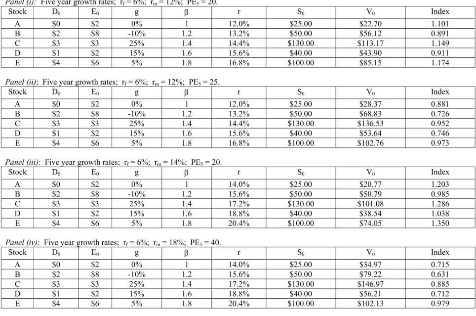
Table 1 presents the valuations of the stocks from Example 2 under several scenarios. In Panel (i), the stocks are valued using rm = 12% and Q = 20. The last column shows a valuation

index for each company. That index is the ratio of the current share price of the stock to our estimate of stock value. The higher is the valuation index, the greater the apparent overpricing. Indexes greater than one indicate apparent overpricings while indexes below one indicate apparent underpricings. Notice that stock B appears to be the most underpriced while stock E appears to be the most overpriced. We say that stock B is underpriced relative to the other stocks while stock E is overpriced relative to the other stocks. Panels (ii) and (iii) present evidence regarding the sensitivity of the calculations to changes in r

5

ˆ

m and Qˆ₅. In Panel (ii), rm = 12% and

= 25. Notice, again, that stock B appears to be the most underpriced while stock E appears to be the least underpriced (most overpriced). In Panel (iii), r

5

ˆ Q

m = 14% and = 20. Again, stock

B appears to be the most underpriced while stock E appears to be the most overpriced. It is not a coincidence that all three panels show the same qualitative result. Because the expected market return and the expected P/E ratio impact each calculation in much the same way, the relative rankings of the stocks are unlikely to change. It is possible, however, for the rank orderings to

5

ˆ Q

(12)

change when stocks have different dividend payout ratios and/or different betas. In those cases, varying the expected P/E ratio or the expected market return will have different impacts on the valuations of the stocks. If mispricing indexes are close to begin with, the relative rankings could change. In such cases, we would conclude that the stocks are similarly mispriced.

Table 1 provides additional evidence supporting the claim that estimates of rm and Q are

relatively unimportant in the analysis, provided that we are comparing different stocks to each other. Notice that when we increase the P/E ratio from 20 to 25 (Panels (i) and (ii)), our valuation of Stock A changes by 25.0%. Similarly, the valuations of Stocks B, C, D, and E change by 22.6%, 20.6%, 22.2%, and 20.7%, respectively. Thus changing the P/E ratio has roughly the same percentage impact on each stock. The change is greatest for Stock A because it does not pay dividends. Similar results are evident when we consider the increase in r

T

ˆ

m from

12% to 14% (Panels (i) and (iii)). The valuations of Stocks A, B, C, D, and E change by –8.5%, -9.5%, -10.7%, -12.2%, and -13.0%, respectively. Again, the percentage change in valuation is similar for the five stocks. As Malkiel (1963) points out, the expected P/E ratio is important for estimating the value of a single stock. We find, however, that it is less important when comparing stocks.

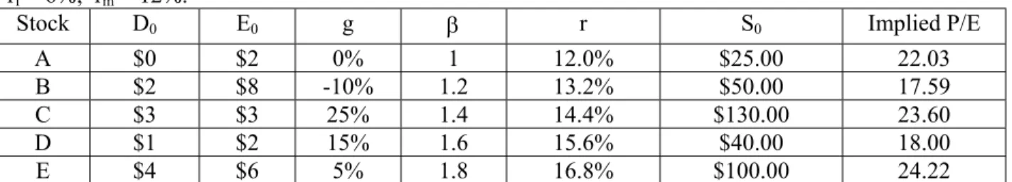
B. Implied Future P/E Ratios for Individual Stocks

An additional application of the model involves calculating implied future P/E ratios for individual stocks or groups of stocks. For individual stocks, one simply calculates the future P/E ratio that would give a valuation equal to the current market price. One can then qualitatively assess the potential mispricing of the stock today by considering the likeliness of achieving that P/E ratio in the future. For example, Stock A in Panel (i) of Table 1 has an implied P/E ratio in

(13)

five years of 22.03. That is, if we value the stock using =22.03, the model provides a valuation of $22.70. To consider the potential mispricing of Stock A, we ask whether 22.03 is a reasonable estimate of the stock’s P/E ratio in five years. Table 2 shows the implied P/E ratios for each of the five stocks of example 2. At the two extremes, stock B has the lowest implied P/E ratio while stock E has the highest. This again suggests that B may be underpriced while E may be overpriced.

5

ˆ Q

C. Implied Future P/E Ratios for Industries

Our technique can be used to calculate an implied future P/E ratio for a given industry. To do this, we choose a future P/E ratio and then calculate current stock values based on that ratio. We then calculate the sum of squared deviations of prices from these values.11 This sum is then minimized by varying the expected P/E ratio to arrive at an implied future P/E ratio.12 The importance of this number is that its reasonableness can be assessed. For example, a 1999 analysis of a group of technology stocks suggested that their implied five-year P/E ratio was 248. The extreme nature of that number suggested that perhaps that group of stocks was overpriced. Subsequent market events confirmed that suggestion.

The implied future P/E ratio for the stocks in Example 2 is 21.28. If we believe this to be unusually high or low, conclusions might be drawn about the desirability of investing in the given industry. In this way, one might use the model to consider industry selection or market timing in general. One could, for example, calculate the implied future P/E ratio for stocks in the S&P 500 index to assess the current level of the index. If the implied ratio is unusually high relative to historical numbers, one might conclude that stocks in general are not wise

(14)

investments. Because the benefits of relative valuation are lost, more care must be used in analyzing industries or the market itself.

III. The Impact of Leverage on P/E Ratios

One premise in our model is that firms in the same industry have the same expected P/E ratio in, say, five years. The motivation for this is that it is extremely difficult to predict what a firm will look like in five years. Consequently, our best guess is that the firm will be average.13 One factor that might cause firms to have different expected P/E ratios is leverage. In the spirit of Modigliani and Miller, replacing some equity with debt would not change the share price of common stock. It might, however, change the earnings per share and thus the P/E ratio. In particular, if the reciprocal of the P/E ratio exceeds the after tax interest rate, then the earnings per share rises (P/E decreases) as leverage increases. If the reciprocal of the P/E is less than the after tax interest rate, then earnings per share decreases (P/E rises) and leverage increases. If the reciprocal of the P/E is equal to the after tax interest rate, then the interest payment reduces earnings by exactly the amount needed to keep earning per share (and P/E) constant when leverage changes.

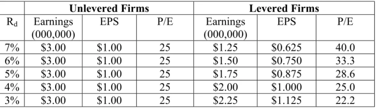
To see this, consider a series of paired firms that are identical except for capital structure. Unlevered firms consist of $75 million in equity and 0 in debt. They have earnings of $3 million and have three million shares outstanding. Thus an unlevered firm has a share price of $25, earnings per share of $1, and a P/E ratio of 25. Levered firms differ from unlevered firms in that $25 million (one million shares) in equity has been replaced by debt. Thus a levered firm has $50 million in equity and $25 million in debt, with two million shares outstanding. The share

(15)

price of a levered firm is $25 (replacing equity with debt does not change the share price), but the earnings are $3 million less the interest payment on debt.

Table 6 shows the earnings per share and P/E ratio for levered firms under varying interest rates. The first row assumes an after-tax cost of debt (denoted Rd) of 7%. A levered firm

therefore pays $1.75 million in interest, which reduces earnings to $1.25 million ($0.625 per share). The levered firm’s P/E is 40.0 in this scenario. It is important to stress that one row in the table is not directly comparable to another row. Since we hold the market value of equity fixed for each type of firm, the unlevered firm with Rd=6% is necessarily a different firm than the

unlevered firm with Rd=4%. The relevant comparison is to contrast the levered firm with the

unlevered firm for a given interest rate. When the cost of debt is 4%, the levered firm’s P/E ratio is 25.0. It is not a coincidence that this is the same P/E ratio as the unlevered firm. When the after-tax cost of debt is equal to the inverse of the P/E ratio, capital structure has no impact on P/E ratios. In that case, higher interest payments from higher levels of debt reduce earnings at exactly the rate necessary to maintain the P/E ratio. When the after-tax cost of debt is less than the reciprocal of the P/E ratio (consider Rd=3% in Table 6, for example), earnings per share

increases (P/E decreases) as leverage increases

The implication of this discussion is that if firms consistently maintain different capital structures, expected P/E ratios will differ. This effect will be eliminated if the after-tax interest rate is equal to the reciprocal of the P/E ratio. Given that we expect firms in the same industry to have similar capital structures, this will often be a minor consideration. However, there can be exceptions.

(16)

IV. Comments on the PEG Ratio

The PEG ratio is typically calculated as the ratio of the current P/E ratio to the earnings growth over a recent period (5 years, for example). Practitioners often cite it as evidence that a stock is mispriced. Peter Lynch, for example, argues that the PEG ratio should be about one for a fairly priced stock. This idea can be explored in the context of our model. First, notice that the historical earnings growth is not directly related to share value. Rather, the anticipated earnings growth is relevant. While the reported PEG ratio is generally based on historical growth rates, the concept could be applied to analysts’ projected growth rates. Second, consider equation (6) while fixing E0, QˆT, and g. V0 is higher when D0 is higher, so if two otherwise identical firms

pay different dividends, the one paying higher dividends should have a higher PEG ratio (V0/g in

our model). V0 is also higher when r (and hence β) is lower. Thus if two otherwise identical

firms have different betas, the one with a higher beta should have a lower PEG ratio. The implication is that firms with identical earnings and earnings growth rates can have different values (even with efficient markets) if their dividend policies differ or if their betas differ. Differences in capital structure might also cause values to differ. This suggests that rules of thumb such as “buy stocks with PEG < 1” are imperfect and may be misleading.

Our analysis is more elaborate than examination of simple PEG ratios. Arguing that stocks should have PEG = 1 would suggest that reducing earnings growth to half its value would reduce share value to half its value. This is approximately true for a zero dividend stock in our model if a 35% growth rate is cut in half. If the growth rate drops from 20% to 10%, however, the stock value only decreases by about 35%. The principle advantage of the PEG ratio is its simplicity, but our model suggests that a more detailed analysis may be appropriate. We argue that the PEG ratio should be used only when comparing groups of stocks with similar dividend

(17)

policies and similar betas, and for which historical earnings growth is likely to be a good proxy for anticipated growth.

V. An Example: Pharmaceuticals

We collected data on October 25, 2000 for several major drug companies. The 5-year Treasury yield was 5.74% on that date.14 This provides an estimate of the risk-free rate. We also gathered data on several major pharmaceutical companies: Eli Lilly (LLY), Pfizer (PFE), Merck (MRK), Johnson and Johnson (JNJ), Bristol Myers Squibb (BMY), and American Home Products (AHP). The general characteristics of these companies are shown in Table 3. Notice that the market capitalizations are similar, suggesting that the optimal capital structures of the firms are likely to be similar. The debt-to-assets ratios vary from 17% to 47%, but we regard the two extremes to be temporary deviations from optimal levels.

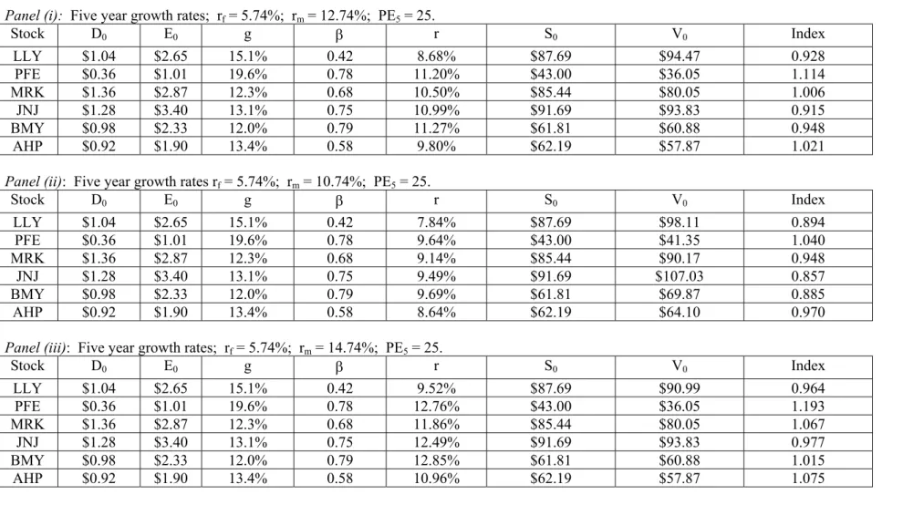
Table 4 reports valuations of these stocks using a market risk premium of 7% and different assumptions on the expected P/E ratio.15 Although the five-year growth rates differ slightly, we have no particular reason to assume that those rates will continue beyond five years. We consequently use the same expected P/E ratio for all the pharmaceutical companies. Panel (i) uses an expected P/E ratio of 25. Notice that Pfizer appears to be the most overpriced while Johnson and Johnson appears to be the most underpriced. Panel (ii) uses an expected P/E ratio of 20 while panel (iii) uses 30. In both cases, Pfizer appears to be the most overpriced while Johnson and Johnson appears to be the most underpriced. We do not conclude that Pfizer is necessarily overpriced. Rather we conclude that Pfizer appears to be overpriced relative to other stocks in the industry. Similarly, we conclude that Johnson and Johnson appears to be underpriced relative to other stocks in the industry. Table 5 reports valuations using a P/E ratio

(18)

of 25 and different assumptions on the expected market return. In all three panels (with market risk premiums of 5%, 7%, and 9%), Pfizer appears to be the most overpriced while Johnson and Johnson appears to be the most underpriced. The consistency of the results in Tables 4 and 5 suggests that the model is robust to changes in both the expected P/E ratio and the expected market return.16

Looking at the debt-to-assets ratios in Table 3, we see a range for pharmaceutical companies from 0.17 to 0.47. These are of course current levels and we might anticipate that they would converge. Furthermore, if the risk-free rate is 5.74%, then the after-tax rate is slightly less than the reciprocal of the P/E ratio (1/25). Since Rd is roughly the same as the

inverse of the P/E ratio, the result is analogous to the 4% line of Table 6. In that line, the levered and unlevered firms have the same P/E ratio. In a Modigliani and Miller (1958) setting in which leverage changes do not change the value of a firm, a change in leverage changes the P/E ratio only when Rd differs from the reciprocal of the P/E ratio. This suggests that adjusting for

leverage would make little difference in this example.

VI. Concluding Comments

We have presented a model that uses P/E ratios, earnings, and earnings growth estimates to estimate fundamental stock values. Our procedure is based on the finite time (typically five years) growth estimates provided by analysts. Although we focus on using earnings, the model might also be applied using sales and price-to-sales ratios. In that way, companies with negative earnings might be valued. The model produces an index of price to value that is useful in comparing companies within a given industry. Although this is our focus, the model might also be used for industry selection or market timing. We also explore how leverage affects our model

(19)

and discuss the implications. An advantage or our method is that it casts discussion in terms of P/E ratios (and their relationship to growth rates) while still preserving much of the analytical reasoning of the discounted dividend model.

(20)

Table 1: Relative Stock Valuation

Panel (i): Five year growth rates; rf = 6%; rm = 12%; PE5 = 20.

E Stock D0 0 g β r S0 V 0 Index A $0 $2 0% 1 12.0% $25.00 $22.70 1.101 B $2 $8 -10% 1.2 13.2% $50.00 $56.12 0.891 C $3 $3 25% 1.4 14.4% $130.00 $113.17 1.149 D $1 $2 15% 1.6 15.6% $40.00 $43.90 0.911 E $4 $6 5% 1.8 16.8% $100.00 $85.15 1.174

Panel (ii): Five year growth rates; rf = 6%; rm = 12%; PE5 = 25.

Panel (iii): Five year growth rates; rf = 6%; rm = 14%; PE5 = 20.

Panel (iv): Five year growth rates; rf = 6%; rm = 18%; PE5 = 40.

(21)

Table 2: Implied P/E Ratios for Individual Stocks rf = 6%; rm = 12%.

Stock D0 E0 g β r S0 Implied P/E

A $0 $2 0% 1 12.0% $25.00 22.03

B $2 $8 -10% 1.2 13.2% $50.00 17.59

C $3 $3 25% 1.4 14.4% $130.00 23.60

D $1 $2 15% 1.6 15.6% $40.00 18.00

E $4 $6 5% 1.8 16.8% $100.00 24.22

Table 3: General Characteristics of Selected Major Drug Companies

Information collected from www.quicken.com. The price-to-earnings ratios are forward looking in that they were computed using expected earnings over the next twelve months.

Company Ticker Market Capitalization ($000,000,000) Price-to-Earnings Ratio Debt-to-Assets Ratio

Eli Lilly LLY $101.2 33.1 0.38

Pfizer PFE $284.9 42.6 0.38

Merck MRK $200.4 29.8 0.35

Johnson and Johnson JNJ $131.7 27.0 0.21

Bristol Myers Squibb BMY $124.9 26.5 0.17

(22)

Table 4: Relative Stock Valuation of Major Drug Companies: Variation of Expected P/E Ratio

Panel (i): Five year growth rates; rf = 5.74%; rm = 12.74%; PE5 = 25.

E Stock D0 0 g β r S0 V 0 Index LLY $1.04 $2.65 15.1% 0.42 8.68% $87.69 $94.47 0.928 PFE $0.36 $1.01 19.6% 0.78 11.20% $43.00 $36.05 1.114 MRK $1.36 $2.87 12.3% 0.68 10.50% $85.44 $80.05 1.006 JNJ $1.28 $3.40 13.1% 0.75 10.99% $91.69 $93.83 0.915 BMY $0.98 $2.33 12.0% 0.79 11.27% $61.81 $60.88 0.948 AHP $0.92 $1.90 13.4% 0.58 9.80% $62.19 $57.87 1.021

Panel (ii): Five year growth rates rf = 5.74%; rm = 12.74%; PE5 = 20.

Panel (iii): Five year growth rates; rf = 5.74%; rm = 12.74%; PE5 = 30.

(23)

Table 5: Relative Stock Valuation of Major Drug Companies: Variation of Expected Market Return

Panel (i): Five year growth rates; rf = 5.74%; rm = 12.74%; PE5 = 25.

Panel (ii): Five year growth rates rf = 5.74%; rm = 10.74%; PE5 = 25.

Panel (iii): Five year growth rates; rf = 5.74%; rm = 14.74%; PE5 = 25.

(24)

Table 6: The Impact of Leverage on P/E Ratios

Unlevered firms have $75 million in equity and 0 in debt. Levered firms have $50 million in equity and $25 million in debt. The share price is $25 for each firm.

Unlevered Firms Levered Firms Rd Earnings

(000,000)

EPS P/E Earnings (000,000) EPS P/E 7% $3.00 $1.00 25 $1.25 $0.625 40.0 6% $3.00 $1.00 25 $1.50 $0.750 33.3 5% $3.00 $1.00 25 $1.75 $0.875 28.6 4% $3.00 $1.00 25 $2.00 $1.000 25.0 3% $3.00 $1.00 25 $2.25 $1.125 22.2

(25)

References

Bodie, Zvi, and Robert C. Merton, Finance, Prentice Hall, 2000.

Brigham, Eugene F. and Joel F. Houston, Fundamentals of Financial Management, Harcourt, Ninth Edition, 2001.

Lakonishok, Josef, Andrei Shleifer, and Robert W. Vishny, “Contrarian Investment, Extrapolation, and Risk,” Journal of Finance 49 no. 5 (December 1994), 1541-1578.

Lynch, Peter and John Rothchild, One Up on Wall Street: How to Use What You Already Know to Make Money in the Market, Simon & Schuster, April 2000.

Malkiel, Burton G., “Equity Yields, Growth, and the Structure of Share Prices,” American Economic Review 53 no. 5 (December 1963), 1004-1031.

Modigliani, Franco and M.H. Miller, “The Cost of Capital, Corporate Finance, and the Theory of Investment,” American Economic Review 48 (June 1958), 261-297.

Van Horne, James C. and John M. Wachowicz Jr., Fundamentals of Financial Management, Prentice Hall, Eleventh Edition, 2001.

(26)

Endnotes

1_{See, for example, Bodie and Merton (2000), Brigham and Houston (2001), and Van Horne and} Wachowicz (2001).

2_{Malkiel (1963) discusses these problems.}

3_{See, for example,}_{www.quicken.com}_{, quote.yahoo.com, and other mainstream finance} websites.

4_{See page 1014.}

5_{It is possible for rank orderings to change when relative mispricings are very close and firms} have significantly different dividend policies. Alternatively, the rank orderings may change when relative mispricings are very close and stocks have significantly different betas.

6_{We present the analysis using earnings and earnings growth rates, but we can adapt the model} to use sales and sales growth rates. In this way, companies with negative earnings (such as many Internet companies) can be valued.

7_{The expected value of}_V

T is equal to the expected value of ET multiplied by the expected value

of QTplus the covariance between ET and QT. We drop the covariance term because it is likely

to be small and we have no easy way to estimate it.

8_{Dividends are typically paid quarterly, with companies changing the dividend amount annually.} Here and throughout the paper, we assume annual dividends to simplify the presentation. The model is easily adapted, however, to account for quarterly dividends.

9_{Note that we discuss the relationship between leverage and P/E ratios in Section III.} 10_{Using a growth phase model would also require an arbitrary adjustment.}

11_{Specifically, we subtract the current price of a stock from its estimated value. We then square} that difference and sum across all stocks in the industry.

12_{Alternatively, a median value might be chosen so that half the population lies above it and half} below it.

13_{Of course if we had reason to believe that a given firm would be above (below) average in five} years, we could simply use a high (low) expected P/E ratio for that firm.

14_{For this illustration, we collected stock information from www.quicken.com and Treasury} security information from FRED database (www.stls.frb.org/fred).

15_{We estimate}_E

0 using analysts’ estimates for the current fiscal year. An implication of this is

(27)

estimated by analysts for that fiscal year. This is an arbitrary choice and one might just as easily use trailing earnings in the model.

16_{Although we do not argue that the model provides predictability, we note that Johnson and} Johnson closed at $107.72 (split-adjusted) on August 10, 2001 while Pfizer closed at $40.75.