Analysis of short term load forecasting techniques / Tan Vy Luoh

Full text

(1)ay. a. ANALYSIS OF SHORT TERM LOAD FORECASTING TECHNIQUES. ity. of. M. al. TAN VY LUOH. U. ni. ve rs. SUBMITTED TO THE GRADUATE SCHOOL OF FACULTY OF ENGINEERING UNIVERSITY OF MALAYA, IN PARTIAL FULFILMENT OF THE REQUIREMENTS FOR THE DEGREE OF MASTER OF POWER SYSTEM ENGINEERING. 2019.

(2) UNIVERSITY OF MALAYA ORIGINAL LITERARY WORK DECLARATION Name of Candidate: TAN VY LUOH Matric No:. KQI170008. Name of Degree:. Master of Power System Engineering. Title of Project Paper/Research Report/Dissertation/Thesis (“this Work”): Analysis of Short Term Load Forecasting Techniques. ay. a. Field of Study: Load Forecasting. I do solemnly and sincerely declare that:. al. I am the sole author/writer of this Work; This Work is original; Any use of any work in which copyright exists was done by way of fair dealing and for permitted purposes and any excerpt or extract from, or reference to or reproduction of any copyright work has been disclosed expressly and sufficiently and the title of the Work and its authorship have been acknowledged in this Work; I do not have any actual knowledge nor do I ought reasonably to know that the making of this work constitutes an infringement of any copyright work; I hereby assign all and every rights in the copyright to this Work to the University of Malaya (“UM”), who henceforth shall be owner of the copyright in this Work and that any reproduction or use in any form or by any means whatsoever is prohibited without the written consent of UM having been first had and obtained; I am fully aware that if in the course of making this Work I have infringed any copyright whether intentionally or otherwise, I may be subject to legal action or any other action as may be determined by UM.. ve rs. (5). ity. (4). of. M. (1) (2) (3). (6). Date:. U. ni. Candidate’s Signature. Subscribed and solemnly declared before, Witness’s Signature. Date:. Name: Designation:. ii.

(3) ABSTRACT. Nowadays, the implementation of advanced technology load and the introduction of multiple renewable energy sources to the grid have created major impacts to the electricity utilities provider with problems of power fluctuation, over generation and conventional power interruption. Therefore, short term load forecasting. a. (STLF) is widely implemented as a necessary technique in power system planning and. ay. operation to ensure the power system is functioning in reliable and secure condition. In this report, three common numerical STLF techniques including Multiple Linear. al. Regression (MLR), Curve Fitting and Bagged Tree Regression are proposed to. M. forecast one-day ahead load profile with a yearly historical load data. The algorithms for each respective techniques are modelled in MATLAB Toolbox for simulation. of. purpose. Forecasted curve of three techniques are obtained for evaluation with the. ity. diagnosis statistics including mean absolute percentage error (MAPE), mean absolute error (MAE), standard deviation absolute percentage error (StdAPE) and standard. ve rs. deviation absolute error (StdAE). The relative error between actual load and forecasted load is computed and used to compare the performance among three STLF techniques. As a result, bagged tree regression has lower relative error in MAPE and StdAPE. ni. which can be used to indicate it is more accurate STLF technique compare to the other. U. two STLF techniques studied in this paper.. iii.

(4) ABSTRAK. Kini, kebanyakan pengunaan alat teknologi modern dan pengunaan pelbagai jenis tenaga boleh baharu telak memainkan peranan penting dalam kehidupan kita serta membawa banyak implikasi kepada pihak penjanaan tenaga elektrik tentang masalah fluktuasi tenaga, kemungkinan untuk menjana sumber tenaga elektrik yang lebih dan gangguan bekalan elektrik. Untuk mengelakkan situasi atas berlaku, model. ay. a. prediksi beban listrik jangka pendek (short term load forecasting) telah dikembangkan dan dilaksanakan dalam proses operasi dan perancangan sistem tenaga elektrik. Dalam. al. projek ini, tiga jenis teknik prediksi iaitu Multiple linear regression, curve fitting dan. M. bagged tree regression telah dikembangkan dengan program komputer MATLAB Toolbox untuk simulasi proses bagi sehari masa tempoh. Keluk yang telah dihasilkan. of. akan dinilai dengan statistik MAPE, MAE, StdAPE dan StdAE. Pembezaan antara. ity. keluk yang telah dihasilkan serta keluk sebenar juga dibangkitkan sebagai ralat yang dapat dibandingkan untuk menilai performasi teknik prediksi. Dapat dibuktikan dari. ve rs. sumber hasil bahawa teknik prediksi bagged tree regression mempunyai ralat yang paling rendah dalam statistik MAPE dan StdAPE serta merujukkan teknik ini lebih. U. ni. akurat berbanding dengan teknik yang dibangkitkan dalam projek ini... iv.

(5) ACKNOWLEDGEMENT. First and foremost, I would like to sincerely appreciate to my supervisor Dr Tan Chia Kwang for his great support and guidance throughout my research project and master study, offering invaluable advice. With his careful supervision and contribution to the direction, this project has done smoothly.. ay. a. Besides, I would also like to acknowledge the lecturers and friends who contributed their. M. knowledge have ease my project’s progress.. al. assistance during the period oy my project. Their kindness on sharing of information and. Finally, I wish to express my deepest thanks to my family for encouraging me all the time. of. especially when I was tough. They have motivated me to continue my project work in. U. ni. ve rs. ity. good performance and always stay far from indolence.. v.

(6) TABLE OF CONTENTS. ABSTRACT ............................................................................................................ ii ABSTRAK ............................................................................................................. iv ACKNOWLEDGEMENT ...................................................................................... v. a. LIST OF FIGURES ............................................................................................... ix. ay. LIST OF TABLES .................................................................................................. x. al. LIST OF SYMBOLS AND ABBREVIATIONS .................................................. xi. M. LIST OF APPENDICES ...................................................................................... xii. of. CHAPTER 1: INTRODUCTION .......................................................................... 1 Background ............................................................................................. 1. 1.2. Problem Statement .................................................................................. 2. 1.3. Objective.................................................................................................. 4. 1.4. Scope and Limitation .............................................................................. 4. 1.5. Outline of Research Report .................................................................... 4. ni. ve rs. ity. 1.1. U. CHAPTER 2: LITERATURE REVIEW ........................................................... 5 2.1. Introduction............................................................................................. 5. 2.2. Short Term Load Forecasting (STLF) Techniques For Existing Power. Planning. ............................................................................................................. 6 2.3. Multiple Linear Regression Technique .................................................10. 2.3.1 Description of Multiple Linear Regression Technique .........................10 vi.

(7) 2.3.2 Estimation of Regression Model Parameter..........................................12 2.4. Curve Fitting Technique ........................................................................14. 2.4.1 Description of Curve Fitting Technique ................................................14 2.4.2 Approach of Curve Fitting to Determine the Best-Fit ..........................15 2.5. Bagged Tree Regression Technique ......................................................17. a. 2.5.1 Classification of Decision Tree...............................................................17. Assessment Method for STLF Method..................................................19. al. 2.6. ay. 2.5.2 Description of Bagged Tree Regression.................................................18. M. 2.6.1 Mean Absolute Percentage Error ..........................................................20. of. 2.6.2 Mean Absolute Error .............................................................................20 2.6.3 Root Mean Squared Error .....................................................................20. ity. 2.6.4 Relative Absolute Error .........................................................................20. ve rs. 2.6.5 Root Relative Squared Error .................................................................21 2.6.6 Standard Deviation of Absolute Percentage Error ...............................21. ni. CHAPTER 3: METHODOLOGY ........................................................................22. U. 3.1. Introduction............................................................................................22. 3.2. Data Pre-processing ...............................................................................23. 3.3. Modelling for Short Term Load Forecasting (STLF) Techniques .......24. 3.3.1 Multiple Linear Regression Technique .................................................24 3.3.2 Curve Fitting Technique ........................................................................25 3.3.3 Bagged Tree Regression Technique ......................................................26. vii.

(8) 3.3.4 Evaluation Metric And Error Analysis .................................................29 3.4. Summary of Chapter .............................................................................30. CHAPTER 4: RESULT AND DISCUSSION .......................................................31 4.1. Introduction............................................................................................31. 4.2. Result of Forecasted Load in STLF.......................................................31. a. 4.2.1 Multiple Linear Regression Technique .................................................31. ay. 4.2.2 Curve Fitting Technique ........................................................................35. al. 4.2.3 Bagged Tree Regression Technique ......................................................38 Performance Evaluation Among STLF Techniques .............................41. 4.4. Summary of Chapter .............................................................................43. of. M. 4.3. CHAPTER 5: CONCLUSION ..............................................................................44 Conclusion ..............................................................................................44. 5.2. Contribution of Research.......................................................................45. 5.3. Recommendations ..................................................................................46. ve rs. ity. 5.1. U. ni. REFERENCES ......................................................................................................47. viii.

(9) LIST OF FIGURES Figure 2.1: Procedure flow chart of regression modelling ............................................12 Figure 3.1: Flow diagram of proposed STLF methodology ..........................................23 Figure 3.2: Flow diagram of bagged tree regression technique .....................................28 Figure 4.1: Comparison of actual load and forecasted load for one day ahead in multiple. a. linear regression technique ..........................................................................................32. ay. Figure 4.2: Relative Error Curve (Multiple Linear Regression) ....................................34. al. Figure 4.3: Comparison of actual load and forecasted load for one day ahead in curve fitting technique ..........................................................................................................35. M. Figure 4.4: Comparison of actual load and forecasted load for one day ahead in curve. of. fitting technique ..........................................................................................................37 Figure 4.5: Comparison of actual load and forecasted load for one day ahead in bagged. ity. tree regression technique .............................................................................................38. ve rs. Figure 4.6: Comparison of actual load and forecasted load for one day ahead in bagged tree regression technique .............................................................................................40. U. ni. Figure 4.7: Comparison of relative error among three STLF techniques.......................41. ix.

(10) LIST OF TABLES. Table 4.1: Regression parameter of multiple linear regression technique .....................32 Table 4.2: Actual, forecast load and absolute percentage relative error for MLR..........33 Table 4.3: Actual, forecast load and absolute percentage relative error for curve fitting. a. ....................................................................................................................................36. ay. Table 4.4: Actual, forecast load and absolute percentage relative error for bagged tree regression ....................................................................................................................39. U. ni. ve rs. ity. of. M. al. Table 4.5 Diagnosis Statistics ......................................................................................41. x.

(11) LIST OF SYMBOLS AND ABBREVIATIONS Artificial Intelligence. ANN. Artificial Neutral Network. ARMA. Autoregressive Moving Average. ARIMA. Autoregressive Integrated Moving Average. CART. Classification And Regression Trees. DS. Decision Stump. LTLF. Long Term Load Forecasting. MAE. Mean Absolute Error. MAPE. Mean Absolute Percentage Error. MLR. Multiple Linear Regression. RE. Renewable Energy. RF. Random Forest. RAE. Relative Absolute Error. ay. al. M. of. ity. Renewable Energy Sources. ve rs. RES. a. AI. Root Mean Square Error. RRSE. Root Relative Squared Error. Reptree. Reduced Error Pruning Tree. SCR. Selective Catalytic Reduction. U. ni. RMSE. SSE. Sum Of Square Error. SVM. Support Vector Machine. xi.

(12) LIST OF APPENDICES Modelling of STLF technique in MATLAB R2015a. U. ni. ve rs. ity. of. M. al. ay. a. APPENDIX A. xii.

(13) CHAPTER 1: INTRODUCTION 1.1. Background Energy crisis is a rising issue all over the world due to the increasing demand. of energy. To cope with this challenge for future development, load forecasting acts as the prominent process for the operation of power system and prepare schedule. ay. a. maintenance plan. Load forecasting basically can be classified into two main categories based on the variety of time horizon: very short term load forecasting. al. (VSTLF), short term load forecasting (STLF), medium term load forecasting (MTLF). M. and long term load forecasting (LTLF). Short term load forecasting usually deals with the load ranging from a couple of hours to one day for load scheduling and generation. of. planning (W. Lee, Jung, & Lee, 2017). Long term load forecasting analyses the load. ve rs. behaviour.. ity. pattern throughout a year or a decade with seasonal weather factor and human. The day-of-day operation of electricity utility system is the main focus for. ni. load forecast thus more approaches are developed for STLF. Every STLF forecasting. U. algorithm has own advantages and drawbacks on data modelling process and assessment of performance (Debnath & Mourshed, 2018). The common challenges of load forecasting are the unexpected weather condition, usage behaviour varies between consumer and misunderstanding of data contributing factors (Kuster, Rezgui, & Mourshed, 2017).. 1.

(14) 1.2. Problem Statement Load forecasting is one of the necessary process for economic and effective. generation of power. Energy suppliers use load forecasting to make optimal unit commitment decision to reduce the spinning reserve capacity and determine the least cost decision which is mainly affected by the load demand and energy purchase.. a. Furthermore, load forecasts is widely used by load serving entitles for system security. ay. and schedule generator operation with well-planned order dispatch. The unexpected. al. variation of the load without accurate load forecasting leads to undesired increase in. M. the reserve capacity. In other word, load forecasting acts as an initial step for electric. of. supplier to schedule an operation decision with economic dispatch consideration.. Besides that, the utility system nowadays is further compounded with. ity. unpredicted renewable energy sources (RES) such as solar, wind, biomass and hydro.. ve rs. Integrating RES to the grid requires sufficient conventional power generation to serve as a backup capacity. Meanwhile, multiple RES injections might impact the cycling of conventional power plants. Cycling can be defined as starting-up, ramping up, ramping. ni. down and shutting down of the power plant generation. In order to cover variable. U. residual demand, the electricity supplier has to control the generation output by ramping or switching on/off the cycling. The changes of operation mode requires long response time and it might cause mismatch between power generation and load demand within the time period.. The accurate STLF optimize the operation scheduling, reduce the cost and supply secure and economical electric energy to the customer. STLF provides the key information for power system scheduling, load flow analysis and day-to day operation 2.

(15) for power delivery and planning. For instance, the residual load demand can be predetermined by the load forecasting technique thus minimize the impact of cycling. During the event of power supply shortage due to intermittence nature of RE, the mismatched load can be covered by the conventional power plant without overestimating or under-estimating and time delay.. a. Based on present researches, there are up to fifteen forecast approaches. ay. applying in energy planning model for short term load forecasting (STLF). Each approaches has its own strength and limitation to generate forecast load with different. al. input parameter. The selection of these various forecast approach will directly affect. M. the forecast result and they can be compared by determine the error between forecasted. of. load and actual load.. ity. In this paper, linear regression, curve fitting and bagged tree regression are used for the STLF of a conventional commercial building to analyse and compare the. ve rs. performance of these three forecast approaches. Real time load data of that particular building is extracted to build a pre-trained data pool for STLF techniques’ training and. U. ni. validation then forecast upcoming 1 day load profile.. 3.

(16) 1.3. Objective. (i). To develop multiple linear regression, curve fitting and bagged tree regression algorithms for short time load forecasting (STLF).. (ii). To analyse the error rate of the developed STLF algorithms using MAPE, MAE STDAPE and STDAE.. (iii). To compare and discuss the performance of the different STLF algorithms in. Among various STLF techniques, this project only discusses three. M. (i). Scope and Limitation. al. 1.4. ay. a. load prediction.. conventional techniques such as linear regression, curve fitting and bagged tree. (ii). of. regression for analysis and evaluation.. The pre-trained load data is purely based on the past load profile from IEEE. All coding and simulation in this report are conducted using MATLAB.. ve rs. (iii). ity. & Kaggle - Global Energy Forecasting Competition 2012 website.. Outline of Research Report. ni. 1.5. U. This report is organized as follows: Chapter 2 presents the literature studies. by other researches which is relevant to this research topic. Chapter 3 develop and study the process of constructing model for simulation and evaluation. Chapter 4 describes the results and discussions for the output achieved from previous chapter . Finally, Chapter 5 summarizes the findings, contribution of research and recommendations for this project.. 4.

(17) CHAPTER 2: LITERATURE REVIEW 2.1. Introduction In present, the global electricity sector is facing multiple power system. planning and operation challenges such as power system resilience issue, the security of supply due to rising of demand and global trend toward urbanization. As bulk electrical energy is not easy to be stored and it aims to be generated wherever there is. a. a demand for it, the power industry is required to estimate the load usage in advance.. al. ay. The process of load estimation in advance is likely to be called as load forecasting.. M. According to the time zone of planning strategy and the power system structure, load forecasting can be categorized into short term load forecasting, medium. of. term load forecasting and long term load forecasting. Each forecast process is executed to predict the load demand for different time horizon with multiple consideration. ity. factors taking in account. With these, the power utility company could generate a. ve rs. comprehensive operation plan to encounter any contingency condition, to make decision on generating and purchasing power and to mitigate the risk related to energy crisis and market economic. As such, a reliable and precise load prediction could ease. U. ni. the participants of market to drive and expand their electricity business.. Short term load forecasting is to serve requisite information for the power. system management of daily operation, fuel resources utilization and unit commitment for the period ranging from hour to week. For different industry practice and location region, there are different load behavior due to the weather condition, nature of business and authority policy. Therefore, multiple variety of short-term load forecasting techniques are developed and refined for precise demand prediction (Singh, Ibraheem, & Muazzam, 2013). Some research studies found that the appropriate 5.

(18) mathematical tool will lead to more accurate forecasting technique when dealing with the randomness on the probabilistic load flow (García-Ascanio & Maté, 2010).. 2.2. Short Term Load Forecasting (STLF) Techniques For Existing Power Planning. Generally, STLF techniques are divided into four categories including. a. statistical, deterministic, artificial intelligence as well as the hybrid technique. For. ay. statistical method, it can be further summarized into regression technique, stochastic time series technique and exponential smoothing technique. The regression-based. al. technique is to predict the relative change of variable by the common relationships. M. derived among the affected variables. Most of the regression algorithm is developed. of. based on weather-dependent factor and socio-economic factor.. ity. Stochastic time series technique can be classified into univariate and multivariate based on either one variable or multiple variables is varying over time.. ve rs. The most common time series technique are curve fitting, autoregressive moving average (ARMA) and autoregressive integrated moving average (ARIMA) (Fengxia & Shouming, 2011). These techniques predict future value based on previous observed. ni. values. Exponential smoothing technique is the advance method of stochastic time. U. series with the use of window function to smooth data instead of moving average.. Aside from statistical techniques, neural network as a part of the artificial intelligent machine learning, it has been employed as the main load forecasting technique which is used extensively in current power system study. The properties of less complicated linear equation and rapid optimization process are the main advantages to support the utility company in optimizing their real-time operation and 6.

(19) saving the investment for any additional facilities construction required especially with the well-development of artificial intelligence (AI) in recent years (Tealab, Hefny, & Badr, 2017). The common topology of neutral network is known as multilayer perceptron which comprises inner layer, multiple hidden layer and output layer (K. Y. Lee, Cha, & Park, 1992). Each layer consists numbers of neuron to represent the set of weights, input variable and the output signal. There are few researches stated that. a. Artificial Neutral Network (ANN) model can be derived with feed forward and back. ay. propagation network (Widodo & Fitriatien, 2016) through using the historical electricity data as the input layer nodes for network training and machine learning in. al. pre-processing stage of load forecasting (Papadopoulos, Delerue, Ryckeghem, &. M. Desmet, 2017).. of. Likewise, the network architecture of neutral network can also be done in. ity. several classes such as recurrent network, radial basis function network and selforganizing maps for clustering (Han, Chen, & Qiao, 2010). The similarity of all neutral. ve rs. network machine learning methods for load forecasting is the repetitive of learning process through feeding the input-output patterns to the network until the convergence of the sum of squared error reach the minimum value. The differences among neutral. ni. network is the selection of activation function and the weights of neuron. Instead of. U. neutral network, the most promising alternative of learning machine algorithm is support vector machine (SVM) which considering statistical learning in pattern classification problems.. Several studies proposed SVM method as the most practical short-term load forecasting due to its capability to solve linear constrained quadratic programming problem (Abbas & Arif, 2006). Moreover, SVM has few significant characteristics. 7.

(20) such as optimal generalization performance, no limitation due to local minima and sparse approximation of solution. There are two main approaches of SVM applied in load forecasting such as non-linear kernel-based method and selective catalytic reduction (SCR) method. Non-linear kernel-based SVM perform classification to take the load data as the input and outputs a line to separate class which is defined as. a. hyperplane (Cocianu, 2013).. ay. All individual STLF technique has its own limitation to handle the challenges of forecasting such as the randomness and non-linear system load, variation. al. of socio-economic environment as well as the weather condition. Conventional load. M. forecasting techniques has their advantages to predict linear load with the historical load data but might lack of accuracy when predict in some particular time zone which. of. is strongly influenced by temperature sensitivities and real time control (Mat Daut et. ity. al., 2017). Therefore, to increase the system reliability, some studies propose the use of hybrid model comprises multiple load-forecasting approaches (Lajevardy, Parand,. ve rs. Rashidi, & Rahimi, 2015).. The combination of time series method and support vector regression is. ni. proposed (Nie, Liu, Liu, & Wang, 2012) while some research combined expert system. U. with neutral network to predict faster and more accurate compare either one of two approaches alone (Wen, Li, Tan, Cao, & Tian, 2015). For instance, this hybrid model could accommodate the performance error occurred from time series method during initiate peak load by using support vector regression while time series method still contributing the seasonal load features and behavior of the load (José Montaño Moreno, Palmer, & Muñoz Gracia, 2011).. 8.

(21) Even though artificial intelligent computing method such as genetic algorithm, neutral network, support vector machine and fuzzy logic are gaining more advantage for their effective use, most of the conventional load forecasting method such as multiple regression, exponential smoothing and stochastic time series are still commonly applying in modern power system especially when the load forecasting trend move toward hybrid model. In fact, the research has been changing and. U. ni. ve rs. ity. of. M. al. ay. a. superseding the old approaches with better performance one.. 9.

(22) 2.3. Multiple Linear Regression Technique 2.3.1 Description of Multiple Linear Regression Technique Multiple linear regression is a statistical attempt to model the linear. relationship between dependent variable and multiple independent variables and it is broadly used in many research fields of economic, natural science and computer science (Amral, Ozveren, & King, 2007). The purpose of multiple linear regression is. a. to evaluate and analyze both linear effect and integrated linear effect of each dependent. ay. variable or independent variables based on the observed data. Once the dependent. al. variable with relative linear impact and independent variables have been chosen, the. M. optimal multiple linear regression algorithm can be created to obtain the deviation degree (Suganthi & Samuel, 2012). As such, one of the major advantages of multiple. of. linear regression is that it capable to resolve multivariate non-linear regression problem through translating the polynomial non-linear regression condition into. ve rs. ity. multiple linear regression (Wang, He, & Nie, 2017).. In the multiple linear regression, the general model with random variable y. and the explanatory variables 𝑥" , 𝑥$, … , 𝑥& which affected the load is expressed in the. U. ni. form as:. 𝑦 = 𝛽+ + 𝛽" 𝑥" + 𝛽$ 𝑥$ + ⋯ + 𝛽& 𝑥& + 𝜀. (1). Where y is the load (the dependent variable), and 𝑥" , 𝑥$, … , 𝑥& are the affecting factor such as weather, time of observation and etc. (k number of independent variables). The independent variables can be controlled and measured through the preprocessing data (Kumar, Mishra, & Gupta, 2016). When k = 1, equation 1 turns into linear regression model; when k is equal or greater 2, equation 1 serves as multiple 10.

(23) linear regression model. An error term 𝜀 is defined in the equation 1 which refer to the undesired noise of the dependent variable y and 𝜀 usually has a mean value equal to zero and constant variance in the case of the probability distributions for the dependent variable y at the various level of the independent variable are in normal distribution as shown in bell shaped. Among equation 1, 𝛽+ , 𝛽" , 𝛽$, … , 𝛽& is k + 1 unknown parameters with 𝛽+ as regression constant while 𝛽" , 𝛽$, … , 𝛽& is partial regression. ay. a. coefficient to be estimated from observation of y and 𝑥& .. Practically, for n sets of data 𝑥/" , 𝑥/$, … , 𝑥/& ; 𝑦/ in term of i = 1, 2, …, n,. M. of. 2014) and written in matrix form,. al. then the linear regression model can be expressed (Ferrera, Hu, Tomasi, & Pastrone,. ity. 𝑦 = 𝑋𝛽 + 𝜀. ve rs. 1 𝑥"" 𝑥"$ 𝑦" 𝑦$ 1 𝑥$" 𝑥$$ Where 𝑦 = 2 5, 𝑋 = 6 ⋮ ⋮ ⋮ ⋮ 𝑦4 1 𝑥4" 𝑥4$. (2). ⋯ 𝑥"& 𝛽+ 𝜀+ ⋮ 𝑥$& 𝜀 𝛽 8, 𝛽 = 6 " 8, 𝜀 = 2 " 5, ⋮ ⋮ ⋮ ⋮ 𝜀4 ⋯ 𝑥4& 𝛽&. ni. Matrix 𝑋 is known as regression data matrix which comprises multiple basic. U. linear regression to facilitate model parameter estimation with n sets of actual observed. data. The predicted value of 𝑦9 is a dependent value with respect to the computed partial regression coefficient parameters 𝑏+ , 𝑏" , 𝑏$, … , 𝑏& are derived from observation of 𝑦. and 𝑋. The predicted value of 𝑦9 is:. 𝑦9 = 𝑏+ + 𝑏" 𝑥" + 𝑏$ 𝑥$ + ⋯ + 𝑏& 𝑥&. (3). 11.

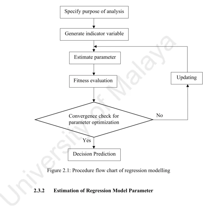
(24) The procedure flow chart of regression model that indicate the methods to obtain a linear correlation coefficient formula is shown in Figure 2.1. Specify purpose of analysis. al. Estimate parameter. ay. a. Generate indicator variable. Updating. of. M. Fitness evaluation. No. ity. Convergence check for parameter optimization. ve rs. Yes. Decision Prediction. ni. Figure 2.1: Procedure flow chart of regression modelling. U. 2.3.2. Estimation of Regression Model Parameter. The most general used method in estimation for unknown regression. parameter after the determination of multiple linear regression model is the ordinary least square method (Patel, Pandya, & Aware, 2015). This method aims to minimize the sum of squared error to get the parameters 𝒃𝒊 , (i = 1, 2, … , k):. [𝒃𝟎 𝒃𝟏 𝒃𝟐 … 𝒃𝒌 ]T = (XT X)-1 XT Y. (4) 12.

(25) Once the regression model parameters are computed, this model can be used for decision prediction, factor analysis and result optimization. For load prediction, the B and the actual load value of y is discrepancy between the predicted load value 𝒚 defined as the residual sum of square (RSS) and the chi-square goodness of fit (R2).. B 𝒊 (𝒕))𝟐 RSS = ∑(𝒚𝒊 (𝒕) − 𝒚. a. 𝒊. (6). al. 𝒊. ay. ∑(𝒚 (𝒕)H𝒚 B (𝒕))𝟐. R2 = 1 - ∑(𝒚𝒊(𝒕)H𝒚I 𝒊(𝒕))𝟐. (5). 𝒚𝒊 (𝒕): Actual load from observation. M. B 𝒊 (𝒕): Estimation load derived from regression method 𝒚. of. I 𝒊 (𝒕): Mean value of actual load 𝒚. ity. Assuming the independent variables have been observed comprehensively. ve rs. and therefore the standard error is minimized. Goodness-of-fit is used to determine the significance of regression parameters where comparing the observed sample distribution with the expected probability distribution (Hong, Gui, Baran, & Willis,. ni. 2010). The closer R2 to 1 indicates that the optimal regression parameters are used to. U. establish the best-fit model for prediction. Hence, the convergence checking for goodness-of-fit value is continuously updating to achieve model optimization. Then, the well-established multiple linear regression model can be utilized to make load prediction (Hahn, Meyer-Nieberg, & Pickl, 2009).. 13.

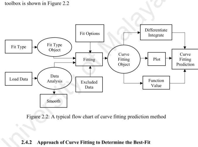
(26) 2.4. Curve Fitting Technique 2.4.1 Description of Curve Fitting Technique. Curve fitting is known as a regression analysis technique which aims to find the best-fit curve for a series of data sample (A Farahat & Talaat, 2012; Jain, Nigam, & Tiwari, 2012). Curve fitting is to establish a parametric equation that able to smooth. a. the data and improve the behavior of plotted graph. Curve fitting technique can be. ay. divided into three common categories such as nonlinear curve fitting, smoothing curve fitting and least squares curve fitting (Molugaram & Rao, 2017). In nonlinear curve. al. fit, researchers are required to specified and customize an equation to be fitted to the. M. data. Generally, nonlinear curve fit is based on the Levenberg-Marquardt algorithm and is simulated using an iterative procedure. During the iteration process, the sum of. of. squared error is calculated and re-evaluated with previous value until it reaches the. ity. best fit.. ve rs. Least squares curve fitting is a technique that minimizes the square of the. error between observed data and the predicted value by the pre-defined equation such as linear, polynomial, power, exponential and logarithmic. Besides, smoothing curve. ni. fits do not require to generate equation for the resulting curve. It uses variety of. U. technique to arrive at the final curve with either incorporating a geometric weight or combining a series of cubic polynomials (Jingfei & Stenzel, 2005). Among three major curve fitting categories, least squares curve fit is the most popular use while nonlinear curve fit is more flexible to fit equation with multiple independent variables.. In most of the technical computing system, curve fitting technique come along with data pre-processing capabilities, pre-defined parametric and nonparametric. 14.

(27) models and also allow the users to customize their own model for specified data analysis (Willis, Powell, & Wall, 1984). Moreover, the integrated curve fitting technique is capable to differential, extrapolate and interpolate the fit during the post processing stage. After the curve fitting equation is built and trained, the curve fit result can be interpreted through correlation coefficients, parameter errors and the sum of the squared error (Chi Square). The typical flow chart of curve fitting prediction method. a. (Reddy Cheepati & Nageswara Prasad, 2016) which is extracted from MATLAB. al. ay. toolbox is shown in Figure 2.2. Fit Type Object. Fit Type. M. Fit Options. Data Analysis. Excluded Data. ity. Load Data. of. Fitting. Differentiate Integrate. Curve Fitting Object. Plot. Curve Fitting Prediction. Function Value. ve rs. Smooth. ni. Figure 2.2: A typical flow chart of curve fitting prediction method. U. 2.4.2 Approach of Curve Fitting to Determine the Best-Fit Several studies have proposed two types of fit results such as goodness of. fit and confidence intervals on the fitted coefficients to identify the accuracy of curve model and the performance for the curve fits the data. In certain cases, in order to reduce error from basic lease square method, orthogonal polynomial curve fitting is proposed (Aman, Simmhan, & Prasanna, 2015; Kafazi, Bannari, Abouabdellah, Aboutafail, & Guerrero, 2017) to make sure all vertical distance square sum between. 15.

(28) every points and fitting curve is minimum. Besides, genetic algorithms which widely used for optimization is proposed to improve the curve model fitting performance with analyzing the Sum of Square Error (SSE) and Root Mean Square Error (RMSE).. For instances, multiple pre-define functions are used as the training model to fit the data and these proposed models are evaluated by RMSE and SSE method.. a. During every iteration, genetic algorithms or support vector regression are. ay. implemented to optimize the coefficients of initial equation then reduce the RMSE. When the RMSE reaches the convergence limit, the best-fit curve is obtained and is. U. ni. ve rs. ity. of. M. al. used to forecast one day ahead load.. 16.

(29) 2.5. Bagged Tree Regression Technique 2.5.1. Classification of Decision Tree. A decision tree is a graphical representation in form of tree structure with internal node that denotes a test on an attribute, branch expresses an outcome of test and leaf node (defined as terminal node) represents the class label (Dudek, 2015). The tree is built in the first stage by recursively splitting the training data into multiple. ay. a. subset based on the assigned optimal criteria. Basically, the construction of tree is completed when all subsets have been assigned the same class label. Then, some. al. algorithms include pruning phase to minimize the outliers and noise that might cause. M. overfitting problem to the data in the decision tree.. of. Generally, there are several kinds of decision tree classification algorithms. ity. including Classification and Regression Trees (CART), Reduced Error Pruning Tree (REPTree), Decision Stump (DS) and Random Forest (RF) proposed for the data. ve rs. mining process of load forecasting (Lahouar & Slama, 2015). Many studies employed and compared the efficiency of the algorithms to determine the best pattern in load forecasting model for the interpretation stage. Among them, CART is the earliest. ni. introduced non-parametric decision tree learning method that works in either. U. classification or regression trees based on the nature of variables. The decision tree of CART is generated based on the valuable value to achieve best split at every node. (Hambali, Akinyemi, Oladunjoye, & N, 2017). REPtree algorithm grew a decision tree with least complexity as it reduces error pruning as well as the error arising from variance. Decision stump is a one-layer decision tree model which purely depending on the single feature value. It is usually used as components in machine learning technique like boosting. A random forest is comprised of a set of decision trees which. 17.

(30) grow the tree in the same way as CART initially. Then, random selection of subset for best split at each node is done iteratively for each of the decision trees.. 2.5.2. Description of Bagged Tree Regression. Bagged tree regression is one of the two ensemble techniques that can be used on the Classification and Regression Trees (CART) to improve the accuracy of. a. decision tree. Ensemble methods including bagging and boosting are defined as a. ay. technique which combines several estimates to construct better predictive performance. al. decision tree (del Carmen Ruiz-Abellón, Gabaldón, & Guillamón, 2018). For bagged. M. tree regression, it is applied with bootstrap aggregation to reduce the variance of estimates. At first, bootstrap aggregation feeds multiple random observations from. of. training set to train multiple models through bootstrap sampling with replacement. Then, all outputs from different fully-grown trees are aggregated into one large model. U. ni. ve rs. ity. then the average of predicted outcome is used for cross validation.. 18.

(31) 2.6. Assessment Method for STLF Method. For load forecast evaluation, there are multiple measures are taken to interpret and compare the prediction model’s performance from various aspects. Some studies focus on the measures of cost, time spend, sensitivity and relationship for decision making through load prediction. There are several comprehensive measures have been proposed to assess load forecasting as a multi-dimensional problem such as. a. scale-independent errors, reliability of model, development cost of model and. al. ay. application independent.. M. Scale-independent error is the most common evaluation measurement which is observed through the difference between the forecasted value and observed. of. value (Zhang et al., 2012). Reliability of model indicates the consistency of model performance to produce similar unseen data relative to the testing data in future.. ity. Meanwhile, the development cost of model is expressed in term of time and effort for. ve rs. data pre-processing, model training and analysing. Application independent measures are based on the comparison across different load forecasting models (Aman et al.,. ni. 2015).. U. Most load forecasting studies evaluate model based on the statistical. measures which can be divided into two main categories: standalone accuracy measures and relative measures. In general, the most used evaluation indicators are Mean Absolute Percentage Error (MAPE), Mean Absolute Error (MAE), Root Mean Squared Error (RMSE), Relative Absolute Error (RAE), Root Relative Squared Error (RRSE) and Standard Deviation Absolute Percentage Error (StdAPE). 19.

(32) 2.6.1. Mean Absolute Percentage Error. The MAPE is scale independent statistical measure that is determined using the absolute error in each period normalized by the observed value in same period then present in percentage form (Khair, Fahmi, Hakim, & Rahim, 2017; W. Lee et al., 2017). This measure is commonly used to determine the error in predicting compare with the. KL HKMN. 4. KL. al. Mean Absolute Error. M. 2.6.2. J x 100%. ay. ". MAPE = ∑ J. a. actual value.. The MAE is scale dependent statistical measure that is computed using the average of. of. absolute error between forecasted load and observed load. ". MAE = ∑|𝑦" − 𝑦′Q |. Root Mean Squared Error. ve rs. 2.6.3. ity. 4. The RMSE is also scale dependent statistical measures which is calculated by taking. ni. the squared root of the average of the squared differences between each forecasted. U. value and its respective actual value (Vazquez et al., 2017).. RMSE = R. 2.6.4. ∑(KL HKMN )S 4. Relative Absolute Error. The RAE is the error that related to the average of the actual values. It is measured by taking the sum of absolute error and normalizes it by dividing by the total absolute error of the average of the actual values. 20.

(33) RAE =. 2.6.5. ∑|KL HKMN | ∑|KMN HKT|. , 𝑦T =. ∑ KMN 4. Root Relative Squared Error. The RRSE is the advanced measures of relative squared error through square root function. ∑(K HKMN )S. RRSE = R ∑( L. , 𝑦T =. ∑ KMN 4. Standard Deviation of Absolute Percentage Error. al. 2.6.6. ay. a. KMN. HKT)S. M. The StdAPE is a measure of volatility to study the spread of forecasted. ity. error, 𝑦9. of. load at each period of time by comparing the relative error with the average relative. ve rs. StdAPE = U. ∑[W. XL YXZN XL. 4H". [HK9]S. ,𝑦9 =. ∑. XL YXZN XL. 4. All above assessment metrics are commonly used to assess STLF techniques. ni. from different perspective. The advantages of MAPE and MAE on assessing STLF are. U. due to their scale-independency and interpretability but the disadvantage is the probability of creating infinite or undefined values for zero (Kim & Kim, 2016).. RMSE has the advantage of penalizing undesirable large error due to it gives a relatively high weight to large errors. Standard deviation is used to indicate the spreading of data compare to the mean in order to determine the system consistency.. 21.

(34) CHAPTER 3: METHODOLOGY 3.1. Introduction This project presents the performance analysis of three numerical short term. load forecast techniques such as multiple linear regression technique, curve fitting technique and bagged tree regression technique. The use of techniques will contribute. a. in different accuracy forecasting result in the same circumstance. To ensure fair. ay. comparison of STLF techniques’ performance, same load data will be extracted and. al. sampled for data processing. Then, the methodology is arranged in the following sequence – data pre-processing, modelling of STLF techniques, scaling and training. M. of load data, simulation and error analysis between forecasted load and actual load to. of. examine the accuracy performance of STLF techniques.. ity. The flow diagram of general methodology is expressed in figure 3.1:. ve rs. Start. Data Analysis and PreProcessing. U. ni. Develop the STLF algorithms Past load data input Forecast the load a day ahead Calculate "MAPE" & "MAE". Result Analysis. End. 22.

(35) Figure 3.1: Flow diagram of proposed STLF methodology 3.2. Data Pre-processing In this project, load data is obtained from the database source from Global. Energy Forecasting Competition 2012 website (IEEE Power & Energy Society, 2012) which comprise hourly load for a year. The dataset containing hourly load from 1 January 2004 to 31 December 2004 are used for training and sampling purpose. Load. a. data of 1 January 2005 is used for leave-one-out cross validation purpose. For each. ay. day, the datasets are separated into twenty-four subset which represent a specific hour. al. of the day. This will allow us to perform comparison analysis between the load of. M. present hour and the load of previous day or week same hour.. of. At the beginning of project, we convert and store the calendar variables of training load dataset into strings comprises year, month, day and hour respectively.. ity. Then, we further categorize the day parameter into corresponding day of week for. ve rs. grouping purpose. Meanwhile, the training loads as well are imported from the dataset and convert into strings according to the time sequence in hour basis. Later, the loads are sort and stored as previous day same hour load, previous week same hour load and. ni. previous twenty-four-hour average load. All missing load data of each category is. U. preset as dummies variable (NaN) before the training process.. Besides, the validation dataset is also converted and stored in string form. The last 24 load data before end of string are sorted and stored into the validated previous day same hour load, validated previous week same hour load and validated previous twenty-four-hour average load to evaluate predictive model. In this case, both training set and testing set are ready to proceed with the next step – modelling of forecast technique. 23.

(36) 3.3. 3.3.1. Modelling for Short Term Load Forecasting (STLF) Techniques. Multiple Linear Regression Technique The implementation of multiple linear regression technique for this. forecasting study is based on hourly load which modelled as two main components. One of the main components is the time of observation which represent the day of week. Another main component is the load for different time period, such as previous. a. week load and previous day load. The relationship between the time of observation. al. ay. and the historical load profile are expressed in multiple linear equation.. M. The multiple linear regression model is expressed as y(t) = 𝛽" 𝑥" + 𝛽$ 𝑥$ + 𝛽] 𝑥] + 𝛽^ 𝑥^. of. Where:. 𝛽" , 𝛽$ , 𝛽] , 𝛽^ = partial regression coefficients. ity. 𝑥" = L (t-24) : represent previous day same hour load. ve rs. 𝑥$ = L (t-720) : represent previous month same hour load ∑NNYS` _ (Q). 𝑥] =. U. ni. 𝑥^ = d. $^. : represent previous day average hour load. : represent day of week (1 to 7 corresponding to Monday to Sunday). Previous day same hour load illustrates the seasonality impacted load which. due to high day and low night temperature as well as human activity at daily resolution. The relationship between load and temperature for monthly resolution can be described and modelled by previous month same hour load due to the variance of weather sensitivity component is reflecting to the load. Day of week is modelled to. 24.

(37) assign the load into respective Mondays to Sundays to analyze the cross effect between the load profile and hour in the particular day (Pahasa & Theera-Umpon, 2007).. The simulation of multiple linear regression is based on the past one-year load profile in hour basic to predict a daily load for one day ahead. The aforementioned four partial regression coefficients are calculated by using the hourly data in respective. a. day of week for every time interval. These parameters are used for cross-validation. ay. with the leave-one-out testing set to forecast a daily load curve which consists the. Curve Fitting Technique. of. 3.3.2. M. al. generalization error estimate.. The implementation of curve fitting is modelled based on nonlinear curve. ity. fit comprises fourier function and root mean square error (RMSE) function. At first, a. ve rs. fourier series equation is created and specified through “fittype” function for the training load data as a data analysis input to create a curve fit. For validation data, we. transform the non-linear daily input into a polynomial sequence with coefficient. U. ni. through regression method.. The fourier equation is described as 𝑓(𝑥 ) = 𝑎+ + 𝑎" cos(𝜔𝑥 ) +. 𝑏" sin (𝜔𝑥). 𝑎+ , 𝑎" 𝑎𝑛𝑑 𝑏" are a dummy coefficient that keep varying until a good fit is obtained. The goodness of fit is based on the RMSE comparing the previous daily load with the present fit model within same hour interval. RMSE states the boundary limitation for the dummy coefficients to converge till the best-fit fourier equation.. 25.

(38) The best fit curve represents a smoothing curve that had trained with the regression coefficient along the entire day range. Then, the predicted load is obtained by considering the trend of the best fit curve and the left-one-out testing sample. For a day, load data is split into 24 hours scatter plot. The vertical distance from the load of the best fit curve interpolates into testing sample to generate the predicted load.. a. The algorithm equation between power and its training parameter is expressed in. ay. y(t) = 𝑎" + 𝑎$ . 𝑃" + 𝑎] . 𝑃$ + 𝑎^ 𝑃]. al. Where:. M. 𝑎" , 𝑎$ , 𝑎] , 𝑎^ : the coefficients derived from the previous load data of similar hour in day, month and the day type. : previous day same hour load. 𝑃$. : previous week same hour load. ity. of. 𝑃". 𝑃]. ve rs. : day type. Bagged Tree Regression Technique. ni. 3.3.3. U. The implementation of bagged tree regression starts from generate predictor. of tree and initiate the prune size for constructing a type of bagged tree technique which is called as random forest. The predictor of tree consists of historical load data. and time of observation. With these training observations, an ensemble of bagged regression tree with specified 50 numbers of weak learner is trained. In random forest technique, weak learner is commonly defined as the input of decision tree for training. The numbers of weak learner determine how accurate and strong the regression tree model can be when combining all of them through ensemble model. 26.

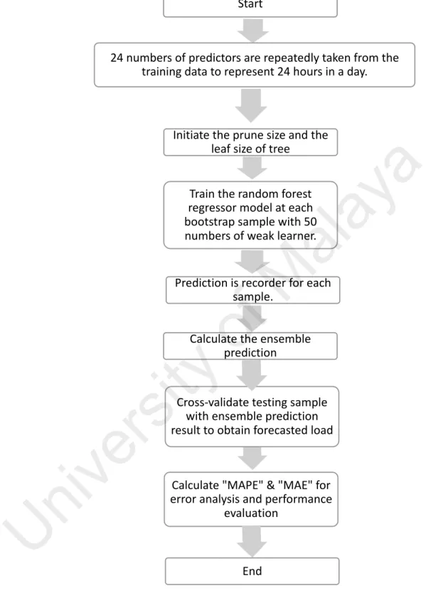
(39) In this paper, the model is built by 24 random forest predictors standing for the 24 hours of the day. The load predictor is affected by few input parameters such as previous day same hour load, previous month same hour load, type of the day, previous 24 hours average load. The output is the load of day at same hour. With these random forest predictors, the regression tree model can predict the 24 coming hours of load. a. demand.. ay. To obtain the optimal size of the tree without overfitting the training data and generate accurate information, the minimum leaf size observation is set as 1 to. al. grow deep tree for large training sample size. Once the regression tree had trained, out-. M. of-sample prediction is used to obtain the validation observation for each of several subtrees. The terminal nodes of the regression tree contain the predicted output. of. variable values. Analyzing through this parameter in each regression tree with the left-. ity. out testing sample, the most accurate cross validated predictions can be produced. In other word, the regression tree is constructed with large number of terminal nodes to. ve rs. optimize the performance of predictor. The flow diagram of bagged tree regression. U. ni. technique is expressed in following figure 3.2:. 27.

(40) Start. 24 numbers of predictors are repeatedly taken from the training data to represent 24 hours in a day.. M. al. ay. Train the random forest regressor model at each bootstrap sample with 50 numbers of weak learner.. a. Initiate the prune size and the leaf size of tree. of. Prediction is recorder for each sample.. ity. Calculate the ensemble prediction. Calculate "MAPE" & "MAE" for error analysis and performance evaluation. U. ni. ve rs. Cross-validate testing sample with ensemble prediction result to obtain forecasted load. End. Figure 3.2: Flow diagram of bagged tree regression technique. 28.

(41) 3.3.4. Evaluation Metric And Error Analysis The evaluation metric is to assess the performance of STLF model through. analyze the error between predicted and actual load. In this report, there are two main error analysis technique had applied such as mean absolute percentage error (MAPE) and mean absolute error (MAE). The error analysis techniques are defined in the. ay. a. following Equation (1) and (2):. ". "++ 4. KN HoN. ∑4Qn" J. KN. J. (1) (2). M. MAPE (𝑦, 𝑝) =. al. MAE (𝑦, 𝑝) = 4 ∑4Qn"|𝑦Q − 𝑝Q |. Where. : actual load value. 𝑝Q. : forecasted load value. n. : number of samples. ity. of. 𝑦Q. : hour. ve rs. t. For each STLF techniques, the forecasted load curve is displayed on a. ni. graphic including all forecasted hour in the validation phase. The forecasted load curve. U. is used to examine the error which reflected in load curve with the actual load curve for a day ahead. The variance of load for each hour is assessed with the average percentage relative error curve.. 29.

(42) 3.4. Summary of Chapter This chapter describes the research methodology used to model STLF. techniques and analyse the data to achieve the research objective. First, data preprocessing introduces the source of load data, transform the raw data into understandable and readable format for coding and modelling tasks. The modelling of three STLF techniques is one of the main research aims to generate consistent and. a. comprehensive system to make the analysis easier to understand and visualize. After. ay. that, the assessment of STLF techniques through simulation is presented. Lastly, the. U. ni. ve rs. ity. of. M. al. error analysis is carried out to examine the performance of STLF techniques.. 30.

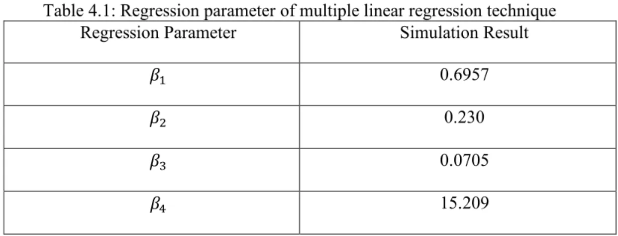
(43) CHAPTER 4: RESULT AND DISCUSSION 4.1. Introduction The chapter first presents the forecasted load curve and actual load curve. for both multiple linear regression technique, curve fitting technique and bagged tree regression technique using MATLAB Toolbox. Then, the result of evaluation metric. a. such as MAPE and MAE are calculated and presented. For each respective technique,. ay. the relative error between forecast load and actual load in per hour basic is presented.. Result of Forecasted Load in STLF. M. 4.2. al. In the last section, the comparison of numerical STLF technique is presented.. of. This section presents the result of the forecasted load in short term load. ve rs. tree regression.. ity. forecasting technique including multiple linear regression, curve fitting and bagged. 4.2.1. Multiple Linear Regression Technique. ni. In this section, the result of multiple linear regression with four input. U. parameters including previous day same hour load, previous month same hour load, previous day average hour load and day of week are presented including the load curve, percentage relative error curve and error metric. The model is derived with the regression parameters which have been calculated using historical hourly load data. These parameters are shown in Table 4.1:. 31.

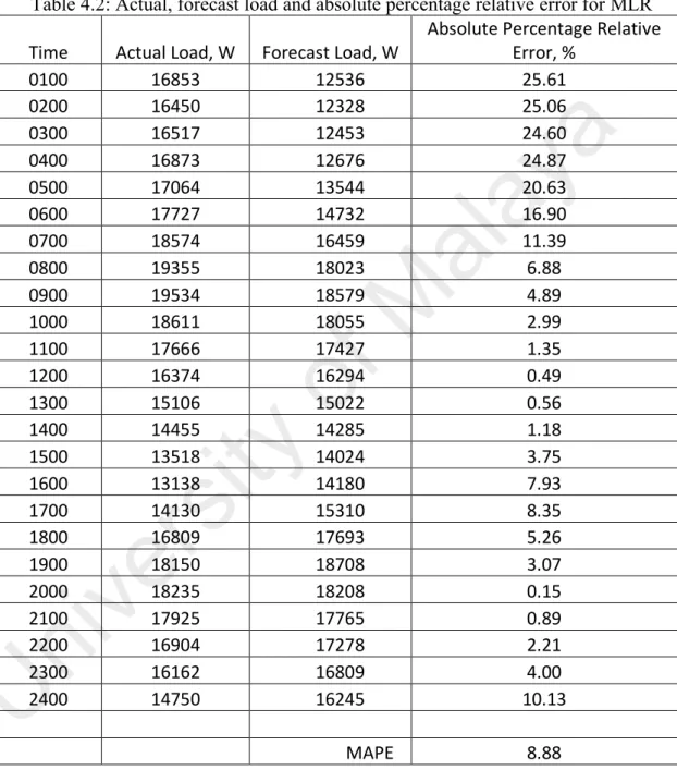
(44) Table 4.1: Regression parameter of multiple linear regression technique Regression Parameter Simulation Result 𝛽". 0.6957. 𝛽$. 0.230. 𝛽]. 0.0705. 𝛽^. 15.209. a. For every hourly time interval, the multiplication of regression parameter. ay. and validation load data generates the forecasted load. The forecasted load against. U. ni. ve rs. ity. of. M. al. actual load for one day ahead are simulated and illustrated in Figure 4.1.. Figure 4.1: Comparison of actual load and forecasted load for one day ahead in multiple linear regression technique To evaluate the performance of MLR technique for STLF, the relative error between forecasted load and actual load are computed and shown in Table 4.2. Besides, the mean absolute percentage error (MAPE) was calculated as 8.88% while 32.

(45) the mean absolute error (MAE) was calculated as 1484.15kW. The percentage relative error curve for MLR is presented in Figure 4.2 to depict the error variation that was generated through MLR.. U. ni. ve rs. ity. of. M. al. ay. a. Table 4.2: Actual, forecast load and absolute percentage relative error for MLR Absolute Percentage Relative Time Actual Load, W Forecast Load, W Error, % 0100 16853 12536 25.61 0200 16450 12328 25.06 0300 16517 12453 24.60 0400 16873 12676 24.87 0500 17064 13544 20.63 0600 17727 14732 16.90 0700 18574 16459 11.39 0800 19355 18023 6.88 0900 19534 18579 4.89 1000 18611 18055 2.99 1100 17666 17427 1.35 1200 16374 16294 0.49 1300 15106 15022 0.56 1400 14455 14285 1.18 1500 13518 14024 3.75 1600 13138 14180 7.93 1700 14130 15310 8.35 1800 16809 17693 5.26 1900 18150 18708 3.07 2000 18235 18208 0.15 2100 17925 17765 0.89 2200 16904 17278 2.21 2300 16162 16809 4.00 2400 14750 16245 10.13 MAPE. 8.88. 33.

(46) a ay al M of. Figure 4.2: Relative Error Curve (Multiple Linear Regression). ity. In figure 4.2, the highest absolute percentage relative error is 25.61%. ve rs. during early morning while the lowest absolute percentage relative error is obtained at night time which is 0.49%. The relative error went down during peak load period and. U. ni. spike up when the load demand drops during off peak period.. 34.

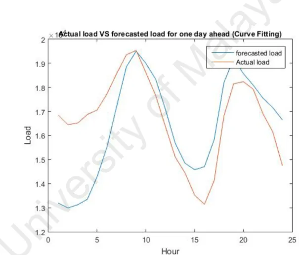
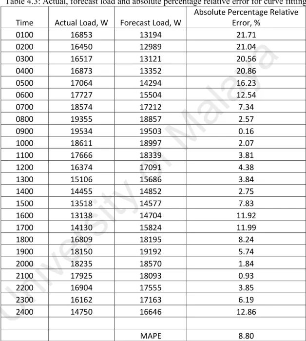
(47) 4.2.2. Curve Fitting Technique In this section, the result of curve fitting which implemented in fourier. equation is presented including the load curve, percentage relative error curve and error metric. The model is based on the “goodness to fit” principle which initially built with the linear regression parameters as the primary input. After few iterations, the best-fit forecasted load against actual load curve for one-day ahead was achieved and. U. ni. ve rs. ity. of. M. al. ay. a. shown in figure 4.3.. Figure 4.3: Comparison of actual load and forecasted load for one day ahead in curve fitting technique. To evaluate the performance of curve fitting technique for STLF, the relative error between forecasted load and actual load are computed and shown in Table 4.3. Besides, the mean absolute percentage error (MAPE) was calculated as 35.

(48) 8.803% while the mean absolute error (MAE) was calculated as 1436.37kW. The percentage relative error curve for curve fitting is presented in Figure 4.4 to depict the error variation that was generated through curve fitting.. U. ni. ve rs. ity. of. M. al. ay. a. Table 4.3: Actual, forecast load and absolute percentage relative error for curve fitting Absolute Percentage Relative Time Actual Load, W Forecast Load, W Error, % 0100 16853 13194 21.71 0200 16450 12989 21.04 0300 16517 13121 20.56 0400 16873 13352 20.86 0500 17064 14294 16.23 0600 17727 15504 12.54 0700 18574 17212 7.34 0800 19355 18857 2.57 0900 19534 19503 0.16 1000 18611 18997 2.07 1100 17666 18339 3.81 1200 16374 17091 4.38 1300 15106 15686 3.84 1400 14455 14852 2.75 1500 13518 14577 7.83 1600 13138 14704 11.92 1700 14130 15824 11.99 1800 16809 18195 8.24 1900 18150 19192 5.74 2000 18235 18570 1.84 2100 17925 18093 0.93 2200 16904 17555 3.85 2300 16162 17163 6.19 2400 14750 16646 12.86 MAPE. 8.80. 36.

(49) a ay al M ity. of. Figure 4.4: Comparison of actual load and forecasted load for one day ahead in curve fitting technique For curve fitting technique, the highest absolute percentage relative error. ve rs. is 21.71% during early morning while the lowest absolute percentage relative error occurred in the late morning at 0.16%. The relative error curve of curve fitting illustrates similar pattern to regression method which varies according to the load. ni. demand. During peak load time, respective lower relative error is obtained especially. U. in the transition period from low load demand to high load demand. In opposite, the relative error goes up and fluctuate between low load usage period.. 37.

(50) 4.2.3. Bagged Tree Regression Technique In this section, the result of bagged tree regression which applied with. ensemble learning method is presented including the load curve, percentage relative error curve and error metric. Multiple weak learners in ensemble term groups together to form a strong learner, so called as random forest. The final result may either be a weighted mean or mean of all of the terminal nodes that are reached. In this case, the. ay. U. ni. ve rs. ity. of. M. al. day ahead was achieved and shown in figure 4.5.. a. optimal forecasted load of bagged tree regression against actual load curve for one-. Figure 4.5: Comparison of actual load and forecasted load for one day ahead in bagged tree regression technique. 38.

(51) To evaluate the performance of bagged tree regression technique for STLF, the relative error between forecasted load and actual load are computed and shown in Table 4.4. Besides, the mean absolute percentage error (MAPE) was calculated as 7.96% while the mean absolute error (MAE) was calculated as 1296.82kW. The percentage relative error curve for bagged tree regression is presented in Figure 4.6 to depict the. a. error variation that was generated through bagged tree regression method.. U. ni. ve rs. ity. of. M. al. ay. Table 4.4: Actual, forecast load and absolute percentage relative error for bagged tree regression Absolute Percentage Relative Time Actual Load, W Forecast Load, W Error, % 0100 16853 14184.91 15.83 0200 16450 13926.96 15.34 0300 16517 13884.27 15.94 0400 16873 13860.32 17.86 0500 17064 14613.74 14.36 0600 17727 15279.52 13.81 0700 18574 17928.36 3.48 0800 19355 18492.66 4.46 0900 19534 18771.71 3.90 1000 18611 17954.35 3.53 1100 17666 18309.70 3.64 1200 16374 16646.33 1.66 1300 15106 15047.82 0.39 1400 14455 15026.53 3.95 1500 13518 14722.64 8.91 1600 13138 14933.39 13.67 1700 14130 15692.78 11.06 1800 16809 17838.04 6.12 1900 18150 18433.18 1.56 2000 18235 18956.86 3.96 2100 17925 18382.17 2.55 2200 16904 17585.97 4.03 2300 16162 16952.34 4.89 2400 14750 17140.40 16.21 MAPE. 7.96. 39.

(52) a ay al M ity. of. Figure 4.6: Comparison of actual load and forecasted load for one day ahead in bagged tree regression technique For tree bagged regression technique, the highest absolute percentage. ve rs. relative error is 15.83% during early morning while the lowest absolute percentage relative error occurred in the late morning at 0.39%.. ni. Due to the characteristic of bagged tree regression method as a random. U. forest, every program execution creates a subset of the data randomly to form a forest. with varies tree size. In addition of the random predictor variables are selected differently from node to node along with the higher possibility of noise, the final. terminal node that is reached might different to the previous execution. Hence, the tree bag regression with random forest algorithm predicts the forecast load through optimization process.. 40.

(53) 4.3. Performance Evaluation Among STLF Techniques Comparing the relative error and mean absolute percentage error for three. discussed STLF techniques, the overall error is close but slightly different from time to time. As it shown in the relative error curve for all three techniques, the index can efficiently evaluate the accuracy of forecast load under the same input load data. The comparative STLF of the load has been tabulated below Table 4.5 to show the variation. Table 4.5 Diagnosis Statistics MAPE StdAPE (%). M. (%). MAE. STDAE. (W). (W). al. STLF Techniques. ay. among three STLF techniques is illustrated in Figure 4.7:. a. of load with respect to the diagnosis statistics and the comparison of relative curve. 8.88. 8.96. 1484.15. 1510.36. Curve Fitting. 8.80. 6.99. 1436.37. 1155.79. 7.96. 5.82. 1296.82. 930.29. U. ni. ve rs. ity. Tree Bagged Regression. of. Multiple Linear Regression. Figure 4.7: Comparison of relative error among three STLF techniques 41.

(54) To have better understanding on the STLF techniques’ performance, we further introduce the standard deviation diagnosis statistic to study how the load data is distributed about the mean value throughout the observation period. From Table 4.5, we know that tree bagged regression generate the forecast load curve with lowest StdAPE and StdAE which indicate that this technique capable to provide the most. ay. a. accurate prediction among three STLF techniques.. Meanwhile, curve fitting and multiple linear regression have a very close. al. MAPE but the multiple linear regression produces a load prediction with greater. M. standard deviation. The reason is mainly due to the wide range of predictor parameter creates white noise and also MLR technique unable to forecast beyond the training. of. data. Thus, the forecasted result may contain unnecessary noise error and the equation. ity. only limited to the particular regression coefficient without cover all affecting factors.. ve rs. For curve fitting technique, the best-fit curve is obtained through fitting. multiple input parameters into the defined fourier equation on top of the basic linear regression. Therefore, the standard deviation of average percentage error seems to be. ni. slightly lower compare to the multiple linear regression technique. In the other words,. U. the number of prediction variable determines how efficient and consistent the. performance of STLF techniques are to generate accurate forecast load curve.. Overall, three STLF techniques have interpreted similar load profile for cross validation. The high relative error which has occurred on the morning and early evening indicate the training data consists numbers of undesired intercorrelation. Moreover, the prediction during the peak load period has the lowest relative error,. 42.

(55) therefore, the forecasted peak load is in high precision. Comparing the diagnosis statistics of numerical STLF techniques that had computed, tree bagged regression has the greater advantage to generate precise load prediction in short term basis.. 4.4. Summary of Chapter In this chapter, the findings of research study are discussed with the. a. simulation result. First of all, the validation result for one day ahead load is presented. ay. in the comparison curve of forecasted load and actual load. Next, the relative error is. al. tabulated and presented in graphical form to analyse the mean absolute percentage. M. error (MAPE) and the mean absolute error (MAE) for all three techniques such as multiple linear regression, curve fitting and bagged tree regression. Besides, the. U. ni. ve rs. ity. StdAE index.. of. performance evaluation with the diagnosis statistic is conducted with StdAPE and. 43.

(56) CHAPTER 5: CONCLUSION 5.1. Conclusion This project serves the purpose of analyse the short term load forecasting. (STLF) techniques and evaluate the performance of respective technique for one day. a. ahead load prediction. The project took one year historical load data as the training. ay. data for load forecasting simulation.. al. First, the load data from Global Energy Forecasting Competition 2012 is. M. extracted and sampled for left-one out cross validation. These data are then stored in excel file in hour basis as time interval to analyse the daily load profile. For three. of. numerical STLF techniques such as multiple linear regression, curve fitting and. ity. bagged tree regression, the respective algorithms are modelled in MATLAB Toolbox with several predictors selected. With this, the objective of STLF technique. ve rs. demonstration had been achieved.. Furthermore, the simulation result that had been obtained through cross. ni. validation comprises of a day ahead forecasted load curve and the relative error. U. between the prediction result and actual load over the time of observation. Evaluating the result allows us to study the characteristic of the STLF techniques and how precise the simulation is done. The key index of MAPE and MAE which determine the error had been generated through simulation. As such, the analysis of each STLF technique had been conducted as Objective 2.. 44.

(57) Last but not least, the comparison findings of numerical STLF techniques’ performance have been analyzed with the statistics results of StdAPE and StdAE. The strength and weakness of each STLF technique had been discussed for a specified period of time ahead. It had concluded that with the same historical data as the training parameter, tree bagged regression had deliberately reflected the best-fit forecasted load result with the lowest error made. Objective 3 which aims to identify the best common. ay. a. practice numerical short-term load forecasting technique has been achieved.. In short, all objectives which had been stated in Chapter 1 have been. M. al. achieved to address the problem statements of this research project.. Contribution of Research. of. 5.2. ity. a) Discovery that the bagged tree regression technique led to optimal. ve rs. advancement for one-day-ahead load prediction. This project had modelled the bagged tree regression which is known as one of the most popular tree-based ensemble machine learning method. The. ni. combination of several weak learner into a decision tree with large leaf size. U. permutate the training data for decision making. The simulation result of proposed predictive ensemble bagged tree regression method indicates it has the good performance to reduce the variance of error. The comparison results revealed that this suggested method could significantly increase the forecast accuracy and reliability in forecasting daily non-linear load profile.. 45.

(58) b) Discovery that the curve fitting technique is highly dependent on the regression coefficient obtained from basic linear regression method. This project had studied the capability of curve fitting technique for short term load forecasting with modelling in MATLAB Toolbox. Even though the interpretation of prediction method differs to the multiple linear regression (MLR) technique, however, the initial predictors are derived in the same way. a. with linear regression method therefore the similar regression coefficients are. ay. obtained at the beginning. The variation between curve fitting and MLR is only the prediction variables are not as straightforward to interpret as linear. Recommendations. of. 5.3. M. al. regression, but provide the best-fit to the specified curve type in our modelling.. This research project had concluded that the capability of multiple linear. ity. regression, curve fitting and bagged tree regression to produce one day ahead. ve rs. forecasting with one year historical load data. Moreover, the consideration factors for data training in this research project are limited to the previous load samples and time of observation. For further research purpose, the modelling with temperature and. ni. weather condition factors can be conducted to explore more reliable and. U. comprehensive result.. Furthermore, the project considered only the conventional load profile throughout the static period of time. Future study for renewable energy environment and advanced electric load can be conducted to analyze the capability of STLF techniques to produce accurate prediction.. 46.

(59) REFERENCES A Farahat, M., & Talaat, M. (2012). A New Approach for Short-Term Load Forecasting Using Curve Fitting Prediction Optimized by Genetic Algorithms (Vol. 2). Abbas, S. R., & Arif, M. (2006, 23-24 Dec. 2006). Electric Load Forecasting Using Support Vector Machines Optimized by Genetic Algorithm. Paper presented at the 2006 IEEE International Multitopic Conference.. a. Aman, S., Simmhan, Y., & Prasanna, V. K. (2015). Holistic Measures for Evaluating. ay. Prediction Models in Smart Grids. IEEE Transactions on Knowledge and Data. al. Engineering, 27(2), 475-488. doi:10.1109/TKDE.2014.2327022. M. Amral, N., Ozveren, C. S., & King, D. (2007, 4-6 Sept. 2007). Short term load forecasting using Multiple Linear Regression. Paper presented at the 2007 42nd International. of. Universities Power Engineering Conference.. Cocianu, C. (2013). Kernel-Based Methods for Learning Non-Linear SVM (Vol. 47).. and. Sustainable. Energy. Reviews,. 88,. 297-325.. ve rs. Renewable. ity. Debnath, K. B., & Mourshed, M. (2018). Forecasting methods in energy planning models.. doi:https://doi.org/10.1016/j.rser.2018.02.002. del Carmen Ruiz-Abellón, M., Gabaldón, A., & Guillamón, A. (2018). Load Forecasting. ni. for a Campus University Using Ensemble Methods Based on Regression Trees. U. (Vol. 11).. Dudek, G. (2015). Short-Term Load Forecasting Using Random Forests. In (Vol. 323, pp. 821-828). Fengxia, Z., & Shouming, Z. (2011, 8-10 Aug. 2011). Time series forecasting using an ensemble model incorporating ARIMA and ANN based on combined objectives. Paper presented at the 2011 2nd International Conference on Artificial Intelligence, Management Science and Electronic Commerce (AIMSEC).. 47.

No results found