Management System
Arvind Arasu, Brian Babcock, Shivnath Babu, John Cieslewicz, Mayur Datar, Keith Ito, Rajeev Motwani, Utkarsh Srivastava, and Jennifer Widom Department of Computer Science, Stanford University
Contact author:[email protected]
1 Introduction
Traditional database management systems are best equipped to run one-timequeries over finite stored data sets. However, many modern applications such as network monitoring, financial analysis, manufacturing, and sensor net-works require long-running, orcontinuous, queries over continuous unbounded streams of data. In the STREAM project at Stanford, we are investigating data management and query processing for this class of applications. As part of the project we are building a general-purpose prototypeData Stream Man-agement System (DSMS), also called STREAM, that supports a large class of declarative continuous queries over continuous streams and traditional stored data sets. The STREAM prototype targets environments where streams may be rapid, stream characteristics and query loads may vary over time, and system resources may be limited.
Building a general-purpose DSMS poses many interesting challenges: • Although we consider streams of structured data records together with
conventional stored relations, we cannot directly apply standard relational semantics to complex continuous queries over this data. In Sect. 2, we describe the semantics and language we have developed for continuous queries over streams and relations.
• Declarative queries must be translated intophysical query plans that are flexible enough to support optimizations and fine-grained scheduling deci-sions. Our query plans, composed ofoperators,queues, andsynopses, are described in Sect. 3.
• Achieving high performance requires that the DSMS exploit possibilities for sharing state and computation within and across query plans. In ad-dition, constraints on stream data (e.g., ordering, clustering, referential integrity) can be inferred and used to reduce resource usage. In Sect. 4, we describe some of these techniques.
• Since data, system characteristics, and query load may fluctuate over the lifetime of a single continuous query, anadaptive approach to query exe-cution is essential for good performance. Our continuous monitoring and reoptimization subsystem is described in Sect. 5.
• When incoming data rates exceed the DSMS’s ability to provide exact results for the active queries, the system should performload-shedding by introducing approximations that gracefully degrade accuracy. Strategies for approximation are discussed in Sect. 6.
• Due to the long-running nature of continuous queries, DSMS administra-tors and users require tools to monitor and manipulate query plans as they run. This functionality is supported by our graphical interface described in Sect. 7.
Many additional problems, including exploiting parallelism and supporting crash recovery, are still under investigation. Future directions are discussed in Sect. 8.
2 The CQL Continuous Query Language
For simple continuous queries over streams, it can be sufficient to use a re-lational query language such as SQL, replacing references to relations with references to streams, and streaming new tuples in the result. However, as continuous queries grow more complex, e.g., with the addition of aggrega-tion, subqueries, windowing constructs, and joins of streams and relations, the semantics of a conventional relational language applied to these queries quickly becomes unclear [3]. To address this problem, we have defined a for-malabstract semantics for continuous queries, and we have designedCQL, a concrete declarative query language that implements the abstract semantics.
2.1 Abstract Semantics
The abstract semantics is based on two data types, streams and relations, which are defined using a discrete, orderedtime domainΓ:
• A stream S is an unbounded bag (multiset) of pairs hs, τi, where s is a tuple andτ ∈Γ is thetimestamp that denotes the logical arrival time of tupleson streamS.
• A relation R is a time-varying bag of tuples. The bag of tuples at time
τ ∈Γ is denotedR(τ), and we callR(τ) aninstantaneous relation. Note that our definition of a relation differs from the traditional one which has no built-in notion of time.
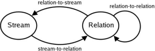
The abstract semantics uses three classes of operators over streams and relations:
Fig. 1.Data types and operator classes in abstract semantics.
• A relation-to-relation operator takes one or more relations as input and produces a relation as output.
• A stream-to-relation operator takes a stream as input and produces a relation as output.
• A relation-to-stream operator takes a relation as input and produces a stream as output.
Stream-to-stream operators are absent—they are composed from operators of the above three classes. These three classes are “black box” components of our abstract semantics: the semantics does not depend on the exact operators in these classes, but only on generic properties of each class. Figure 1 summarizes our data types and operator classes.
A continuous queryQis a tree of operators belonging to the above classes. The inputs of Q are the streams and relations that are input to the leaf operators, and the output ofQis the output of the root operator. The output is either a stream or a relation, depending on the class of the root operator. At timeτ, an operator ofQlogically depends on its inputs up toτ: tuples of
Si with timestamps≤τfor each input streamSi, and instantaneous relations
Rj(τ0),τ0 ≤τ, for each input relationRj. The operator produces new outputs
corresponding toτ: tuples ofS with timestampτ if the output is a streamS, or instantaneous relationR(τ) if the output is a relationR. The behavior of queryQ is derived from the behavior of its operators in the usual inductive fashion.
2.2 Concrete Language
Our concrete declarative query language,CQL (forContinuous Query Lan-guage), is defined by instantiating the operators of our abstract semantics. Syntactically, CQL is a relatively minor extension to SQL.
Relation-to-Relation Operators in CQL
CQL uses SQL constructs to express its relation-to-relation operators, and much of the data manipulation in a typical CQL query is performed using these constructs, exploiting the rich expressive power of SQL.
Stream-to-Relation Operators in CQL
The stream-to-relation operators in CQL are based on the concept of asliding window [5] over a stream, and are expressed using a window specification language derived from SQL-99:
• A tuple-based sliding window on a stream S takes an integer N > 0 as a parameter and produces a relationR. At time τ, R(τ) contains the N tuples ofS with the largest timestamps ≤τ. It is specified by following
S with “[Rows N].” As a special case, “[Rows Unbounded]” denotes the append-only window “[Rows ∞].”
• A time-based sliding window on a stream S takes a time intervalω as a parameter and produces a relationR. At timeτ,R(τ) contains all tuples ofS with timestamps betweenτ−ω andτ. It is specified by followingS with “[Range ω].” As a special case, “[Now]” denotes the window with
ω= 0.
• Apartitioned sliding windowon a streamS takes an integerN and a set of attributes{A1, . . . , Ak}ofSas parameters, and is specified by followingS with “[Partition By A1,...,Ak Rows N].” It logically partitionsSinto
different substreams based on equality of attributesA1, . . . , Ak, computes a tuple-based sliding window of sizeN independently on each substream, then takes the union of these windows to produce the output relation.
Relation-to-Stream Operators in CQL
CQL has three relation-to-stream operators:Istream,Dstream, and Rstream. Istream (for “insert stream”) applied to a relationRcontainshs, τiwhenever tuple s is in R(τ)−R(τ−1), i.e., whenever s is inserted intoR at time τ. Dstream(for “delete stream”) applied to a relationRcontainshs, τiwhenever tuple s is in R(τ−1)−R(τ), i.e., whenever s is deleted fromR at time τ. Rstream (for “relation stream”) applied to a relation R contains the hs, τi whenever tuplesis inR(τ), i.e., every current tuple inRis streamed at every time instant.
Example CQL Queries
Example 1.The following continuous query filters a streamS:
Select Istream(*) From S [Rows Unbounded] Where S.A > 10 StreamSis converted into a relation by applying an unbounded (append-only) window. The relation-to-relation filter “S.A > 10” acts over this relation, and the inserts to the filtered relation are streamed as the result. CQL includes a number of syntactic shortcuts and defaults for convenience, which permit the above query to be rewritten in the following more intuitive form:
Select * From S Where S.A > 10
Example 2.The following continuous query is awindowed joinof two streams
S1 andS2:
Select * From S1 [Rows 1000], S2 [Range 2 Minutes] Where S1.A = S2.A And S1.A > 10
The answer to this query is a relation. At any given time, the answer relation contains the join (on attribute Awith A >10) of the last 1000 tuples of S1 with the tuples of S2 that have arrived in previous 2 minutes. If we prefer instead to produce a stream containing new A values as they appear in the join, we can write “Istream(S1.A)” instead of “*” in the Selectclause. Example 3.The following continuous query probes a stored tableRbased on each tuple in streamS and streams the result.
Select Rstream(S.A, R.B) From S [Now], R Where S.A = R.A Complete details of CQL including syntax, semantic foundations, syntactic shortcuts and defaults, equivalences, and a comparison against related con-tinuous query languages are given in [3].
3 Query Plans and Execution
When a continuous query specified in CQL is registered with the STREAM system, a query plan is compiled from it. Query plans are composed of op-erators, which perform the actual processing,queues, which buffer tuples (or references to tuples) as they move between operators, and synopses, which store operator state.
3.1 Operators
Recall from Sect. 2 that there are two fundamental data types in our query language: streams, defined as bags of tuple-timestamp pairs, and relations, defined as time-varying bags of tuples. We unify these two types in our imple-mentation as sequences of timestamped tuples, where each tuple additionally is flagged as either an insertion (+) ordeletion (−). We refer to the tuple-timestamp-flag triples aselements.
Streams only include + elements, while relations may include both + and−elements to capture the changing relation state over time. Queues log-ically contain sequences of elements representing either streams or relations. Each query plan operator reads from one or more input queues, processes the input based on its semantics, and writes any output to an output queue. Individual operators may materialize their relational inputs in synopses (see Sect. 3.3) if such state is useful.
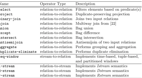
Name Operator Type Description
select relation-to-relation Filters elements based on predicate(s) project relation-to-relation Duplicate-preserving projection binary-join relation-to-relation Joins two input relations mjoin relation-to-relation Multiway join from [22] union relation-to-relation Bag union
except relation-to-relation Bag difference intersect relation-to-relation Bag intersection
antisemijoin relation-to-relation Antisemijoin of two input relations aggregate relation-to-relation Performs grouping and aggregation duplicate-eliminate relation-to-relation Performs duplicate elimination seq-window stream-to-relation Implements time-based, tuple-based,
and partitioned windows i-stream relation-to-stream ImplementsIstreamsemantics d-stream relation-to-stream ImplementsDstream semantics r-stream relation-to-stream ImplementsRstreamsemantics
Table 1.Operators used in STREAM query plans.
The operators in the STREAM system that implement the CQL language are summarized in Table 1. In addition, there are several system operators to handle “housekeeping” tasks such as marshaling input and output and connecting query plans together. During execution, operators are scheduled individually, allowing for fine-grained control over queue sizes and query la-tencies. Scheduling algorithms are discussed later in Sect. 4.3.
3.2 Queues
A queue in a query plan connects its “producing” plan operator OP to its “consuming” operatorOC. At any time a queue contains a (possibly empty)
collection of elements representing a portion of a stream or relation. The elements that OP produces are inserted into the queue and buffered there
until they are processed byOC.
Many of the operators in our system require that elements on their input queues be read in nondecreasing timestamp order. Consider, for example, a window operatorOW on a streamSas described in Sect. 2.2. IfOW receives an elemenths, τ,+iand its input queue is guaranteed to be in nondecreasing timestamp order, thenOW knows it has received all elements with timestamp
τ0 < τ, and it can construct the state of the window at timeτ−1. (If
times-tamps are known to be unique it can construct the state at time τ.) If, on the other hand,OW does not have this guarantee, it can never be sure it has enough information to construct any window correctly. Thus, we require all queues to enforce nondecreasing timestamps.
Mechanisms for buffering tuples and generatingheartbeatsto ensure non-decreasing timestamps, without sacrificing correctness or completeness, are discussed in detail in [17].
3.3 Synopses
Logically, asynopsisbelongs to a specific plan operator, storing state that may be required for future evaluation of that operator. (In our implementation, synopses are shared among operators whenever possible, as described later in Sect. 4.1.) For example, to perform a windowed join of two streams, the join operator must be able to probe all tuples in the current window on each input stream. Thus, the join operator maintains one synopsis (e.g., a hash table) for each of its inputs. On the other hand, operators such as selection and duplicate-preserving union do not require any synopses.
The most common use of a synopsis in our system is to materialize the current state of a (derived) relation, such as the contents of a sliding win-dow or the relation produced by a subquery. Synopses also may be used to store a summary of the tuples in a stream or relation for approximate query answering, as discussed later in Sect. 6.2.
Performance requirements often dictate that synopses (and queues) must be kept in memory, and we tacitly make that assumption throughout this chapter. Our system does support overflow of these structures to disk, al-though currently it does not implement sophisticated algorithms for minimiz-ing I/O when overflow occurs, e.g., [20].
3.4 Example Query Plan
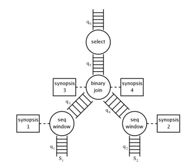
When a CQL query is registered, STREAM constructs a query plan: a tree of operators, connected by queues, with synopses attached to operators as needed. As a simple example, a plan for the query from Example 2 is shown in Figure 2. The original query is repeated here for convenience:
Select * From S1 [Rows 1000], S2 [Range 2 Minutes] Where S1.A = S2.A And S1.A > 10
There are four operators in the example plan: aselect, a binary-join, and one instance of seq-window for each input stream. Queues q1 and q2
hold the input stream elements which could, for example, have been re-ceived over the network and placed into queues by a system operator (not de-picted). Queueq3, which is the output queue of the (stream-to-relation) opera-torseq-window, holds elements representing the relation “S1 [Rows 1000].” Queueq4 holds elements for “S2 [Range 2 Minutes].” Queue q5 holds ele-ments for the joined relation “S1 [Rows 1000]./S2 [Range 2 Minutes],” and from these elements, Queueq6holds the elements passing theselect op-erator.q6may lead to an output operator sending elements to the application, or to another query plan operator within the system.
Theselectoperator can be pushed down into one or both branches be-low the binary-joinoperator, and also below the seq-windowoperator on
Fig. 2.A simple query plan illustrating operators, queues, and synopses.
and therefore theselect operator cannot be pushed below the seq-window operator onS1.
The plan has four synopses,synopsis1–synopsis4. Eachseq-window op-erator maintains a synopsis so that it can generate “−” elements when tuples expire from the sliding window. Thebinary-joinoperator maintains a syn-opsis materializing each of its relational inputs for use in performing joins with tuples on the opposite input, as described earlier. Since theselectoperator does not need to maintain any state, it does not have a synopsis.
Note that the contents ofsynopsis1andsynopsis3are similar (as are the contents ofsynopsis2 andsynopsis4), since both maintain a materialization of the same window, but at slightly different positions of streamS1. Sect. 4.1 discusses how we eliminate such redundancy.
3.5 Query Plan Execution
When a query plan is executed, ascheduler selects operators in the plan to execute in turn. The semantics of each operator depends only on the times-tamps of the elements it processes, not on system or “wall-clock” time. Thus, the order of execution has no effect on the data in the query result, although it can affect other properties such as latency and resource utilization. Scheduling is discussed further in Sect. 4.3.
Continuing with our example from the previous section, theseq-window operator onS1, on being scheduled, reads stream elements fromq1. Suppose it reads elemenths, τ,+i. It inserts tuplesintosynopsis1, and if the window
is full (i.e., the synopsis already contains 1000 tuples), it removes the earliest tuple s0 in the synopsis. It then writes output elements intoq3: the element hs, τ,+ito reflect the addition ofsto the window, and the elemenths0, τ,−i to reflect the deletion of s0 as it exits the window. Both of these events oc-cur logically at the same time instant τ. The other seq-windowoperator is analogous.
When scheduled, the binary-join operator reads the earliest element across its two input queues. If it reads an element hs, τ,+i from q3, then it insertssintosynopsis3and joinsswith the contents ofsynopsis4, generating output elements hs·t, τ,+ifor each matching tuple tin synopsis4. Similarly, if the binary-joinoperator reads an elemenths, τ,−ifrom q3, it generates hs·t, τ,−ifor each matching tupletinsynopsis4. A symmetric process occurs for elements read fromq4. In order to ensure that the timestamps of its output elements are nondecreasing, thebinary-joinoperator must process its input elements in nondecreasing timestamp order across both inputs.
Since the selectoperator is stateless, it simply dequeues elements from
q5, tests the tuple against its selection predicate, and enqueues the identical
element intoq6 if the test passes, discarding it otherwise.
4 Performance Issues
In the previous section we introduced the basic architecture of our query pro-cessing engine. However, simply generating the straightforward query plans and executing them as described can be very inefficient. In this section, we dis-cuss ways in which we improve the performance of our system by eliminating data redundancy (Sect. 4.1), selectively discarding data that will not be used (Sect. 4.2), and scheduling operators to most efficiently reduce intermediate state (Sect. 4.3).
4.1 Synopsis Sharing
In Sect. 3.4, we observed that multiple synopses within a single query plan may materialize nearly identical relations. In Figure 2, synopsis1 and synopsis3 are an example of such a pair.
We eliminate this redundancy by replacing the two synopses with light-weightstubs, and a singlestore to hold the actual tuples. These stubs imple-ment the same interfaces as non-shared synopses, so operators can be oblivi-ous to the details of sharing. As a result, synopsis sharing can be enabled or disabled on the fly.
Since operators are scheduled independently, it is likely that operators sharing a single synopsis store will require slightly different views of the data. For example, if queue q3 in Figure 2 contains 10 elements, then synopsis3
will not reflect these changes (since the binary-joinoperator has not yet processed them), althoughsynopsis1will. When synopses are shared, logic in
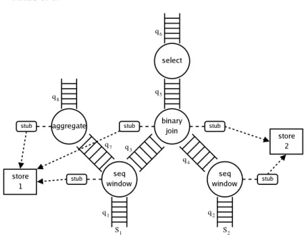
Fig. 3.A query plan illustrating synopsis sharing.
the store tracks the progress of each stub, and presents the appropriate view (subset of tuples) to each of the stubs. Clearly the store must contain the union of its corresponding stubs: A tuple is inserted into the store as soon as it is inserted by any one of the stubs, and it is removed only when it has been removed from all of the stubs.
To further decrease state redundancy, multiple query plans involving sim-ilar intermediate relations can share synopses as well. For example, suppose the following query is registered in addition to the query in Sect. 3.4:
Select A, Max(B) From S1 [Rows 200] Group By A
Since sliding windows are contiguous in our system, the window onS1 in this query is a subset of the window on S1 in the other query. Thus, the same data store can be used to materialize both windows. The combination of the two query plans with both types of sharing is illustrated in Figure 3.
4.2 Exploiting Constraints
Streams may exhibit certain data or arrival patterns that can be exploited to reduce run-time synopsis sizes. Such constraints can either be specified explicitly at stream-registration time, or inferred by gathering statistics over time [6]. (An alternate and more dynamic technique is for the streams to contain punctuations, which specify run-time constraints that also can be used to reduce resource requirements [21].)
As a simple example, consider a continuous query that joins a stream Orders with a streamFulfillments based on attributes orderID and itemID, perhaps to monitor average fulfillment delays. In the general case, answering this query precisely requires synopses of unbounded size [2]. However, if we know that all elements for a givenorderID anditemIDarrive onOrdersbefore the corresponding elements arrive onFulfillments, then we need not maintain a join synopsis for theFulfillmentsoperand at all. Furthermore, ifFulfillments elements arrive clustered by orderID, then we need only saveOrders tuples for a givenorderID until the nextorderID is seen.
We have identified several types of useful constraints over data streams. Effective optimizations can be made even when the constraints are not strictly met by defining anadherence parameter,k, that captures how closely a given stream or pair of streams adheres to a constraint of that type. We refer to these ask-constraints:
• A referential integrity k-constraint on a many-one join between streams defines a boundkon the delay between the arrival of a tuple on the “many” stream and the arrival of its joining “one” tuple on the other stream. • Anordered-arrivalk-constrainton a stream attributeS.Adefines a bound
k on the amount of reordering in values of S.A. Specifically, given any tuple s in stream S, for all tuples s0 that arrive at least k+ 1 elements afters, it must be true thats0.A≥s.A.
• Aclustered-arrivalk-constraint on a stream attributeS.Adefines a bound
kon the distance between any two elements that have the same value of
S.A.
We have developed query plan construction and execution algorithms that take stream constraints into account in order to reduce synopsis sizes at query operators by discarding unnecessary state [9]. The smaller the value of kfor each constraint, the more state that can be discarded. Furthermore, if an assumedk-constraint is not satisfied by the data, our algorithm produces an approximate answer whose error is proportional to the degree of deviation of the data from the constraint.
4.3 Operator Scheduling
An operator consumes elements from its input queues and produces elements on its output queue. Thus, the global operator scheduling policy can have a large effect on memory utilization, particularly with bursty input streams.
Consider the following simple example. Suppose we have a query plan with two operators,O1 followed byO2. Assume that O1 takes one time unit to process a batch of n elements, and it produces 0.2noutput elements per input batch (i.e., itsselectivityis 0.2). Further, assume thatO2takes one time unit to operate on 0.2nelements, and it sends its output out of the system. (As far as the system is concerned,O2 produces no elements, and therefore
its selectivity is 0.) Consider the following bursty arrival pattern:nelements arrive at every time instant fromt= 0 tot= 6, then no elements arrive from timet= 7 throught= 13.
Under this scenario, consider the following scheduling strategies:
• FIFO scheduling: When batches of n elements have been accumulated, they are passed through both operators in two consecutive time units, during which no other element is processed.
• Greedy scheduling: At any time instant, if there is a batch of nelements buffered before O1, it is processed in one time unit. Otherwise, if there are more than 0.2n elements buffered beforeO2, then 0.2nelements are processed using one time unit. This strategy is “greedy” since it gives preference to the operator that has the greatest rate of reduction in total queue size per unit time.
The following table shows the expected total queue size for each strategy, where each table entry is a multiplier forn.
Time 0 1 2 3 4 5 6 Avg
FIFO scheduling 1.0 1.2 2.0 2.2 3.0 3.2 4.0 2.4 Greedy scheduling 1.0 1.2 1.4 1.6 1.8 2.0 2.2 1.6
After timet= 6, input queue sizes for both strategies decline until they reach 0 after timet= 13. The greedy strategy performs better because it runsO1 whenever it has input, reducing queue queue size by 0.8nelements each time step, while the FIFO strategy alternates between executingO1andO2.
However, the greedy algorithm has its shortcomings. Consider a plan with operatorsO1,O2, andO3.O1produces 0.9nelements perninput elements in one time unit,O2processes 0.9nelements in one time unit without changing the input size (i.e., it has selectivity 1), and O3 processes 0.9n elements in one time unit and sends its output out of the system (i.e., it has selectivity 0). Clearly, the greedy algorithm will prioritizeO3first, followed by O1, and thenO2. If we consider the arrival pattern in the previous example then our total queue size is as follows (again as multipliers forn):
Time 0 1 2 3 4 5 6 Avg
FIFO scheduling 1.0 1.9 2.9 3.0 3.9 4.9 5.0 3.2 Greedy scheduling 1.0 1.9 2.8 3.7 4.6 5.5 6.4 3.7
In this case, the FIFO algorithm is better. Under the greedy strategy, although O3 has highest priority, sometimes it is “blocked” from running because it is preceded byO2, the operator with the lowest priority. IfO1,O2
and O3 are viewed as a single block, then together they reduce n elements to zero elements over three units of time, for an average reduction of 0.33n elements per unit time—better than the reduction rate of 0.1nelements O1 provides. Since the greedy algorithm considers individual operators only, it does not take advantage of this fact.
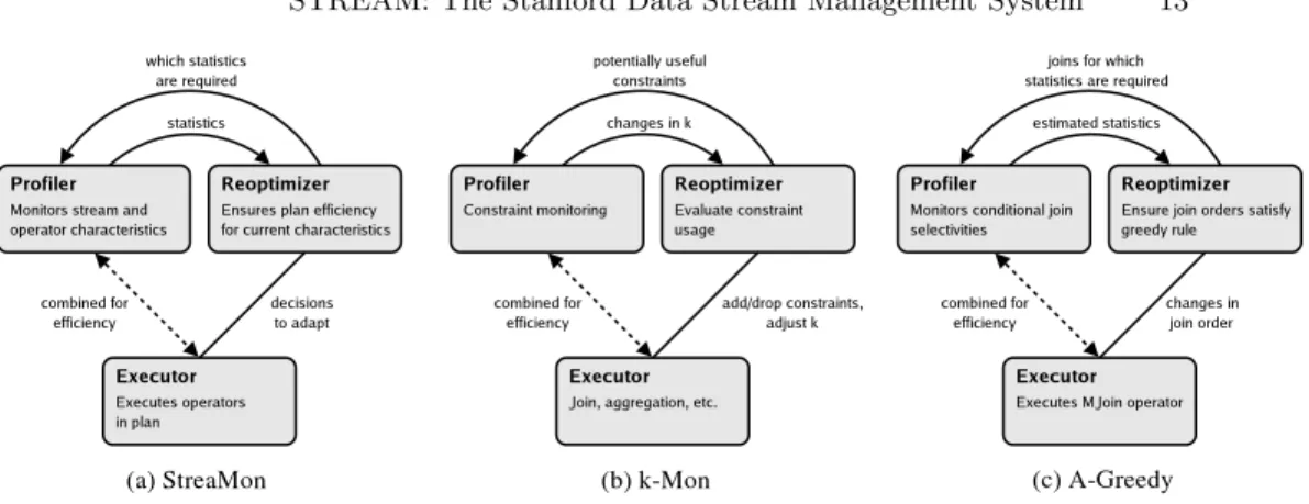
Fig. 4. Adaptive query processing.
This observation forms the basis of ourchain scheduling algorithm [4]. Our algorithm forms blocks (“chains”) of operators as follows: Start by marking the first operator in the plan as the “current” operator. Next, find the block of consecutive operators starting at the “current” operator that maximizes the reduction in total queue size per unit time. Mark the first operator fol-lowing this block as the “current” operator and repeat the previous step until all operators have been assigned to chains. Chains are scheduled according to the greedy algorithm, but within a chain, execution proceeds in FIFO or-der. In terms of overall memory usage, this strategy is provably close to the optimal “clairvoyant” scheduling strategy, i.e., the optimal strategy based on knowledge of future input [4].
5 Adaptivity
In long-running stream applications, data and arrival characteristics of streams may vary significantly over time [13]. Query loads and system conditions may change as well. Without anadaptive approach to query processing, per-formance may drop drastically over time as the environment changes. The STREAM system includes a monitoring and adaptive query processing in-frastructure calledStreaMon [10].
StreaMon has three components as shown in Figure 4(a): an Executor, which runs query plans to produce results, a Profiler, which collects and maintains statistics about stream and plan characteristics, and aReoptimizer, which ensures that the plans and memory structures are the most efficient for current characteristics. In many cases, we combine the profiler and executor to reduce the monitoring overhead.
The Profiler and Reoptimizer are essential for adaptivity, but they compete for resources with the Executor. We have identified a clear three-way tradeoff among run-time overhead, speed of adaptivity, and provable convergence to
good strategies if conditions stabilize. StreaMon supports multiple adaptive algorithms that lie at different points along this tradeoff spectrum.
StreaMon can detect usefulk-constraints (recall Sect. 4.2) in streams and exploit them to reduce memory requirements for many continuous queries. In addition, it can adaptively adjust the adherence parameterkbased on the actual data in the streams. Figure 4(b) shows the portions of StreaMon’s Pro-filer and Reoptimizer that handle k-constraints, referred to ask-Mon. When a query is registered, the optimizer notifies the profiler of potentially useful constraints. As the executor runs the query, the profiler monitors the input streams continuously and informs the reoptimizer whenever it detects a change in a kvalue for any of these constraints. The reoptimizer component adapts to these changes by adding or dropping constraints used by the executor and adjustingk values used for memory allocation.
StreaMon also implements an algorithm called Adaptive Greedy (or A-Greedy) [7], which maintains join orders adaptively for pipelined multiway stream joins, also known as MJoins [22]. Figure 4(c) shows the portions of StreaMon’s Profiler and Reoptimizer that comprise the A-Greedy algo-rithm. Using A-Greedy, StreaMon monitors conditional selectivities and or-ders stream joins to minimize overall work in current conditions. In addition, StreaMon detects when changes in conditions may have rendered current derings suboptimal, and reorders in those cases. In stable conditions, the or-derings converged on by the A-Greedy algorithm are equivalent to those se-lected by a static Greedy algorithm that is provably within a cost factor<4 of optimal. In practice, the Greedy algorithm, and therefore A-Greedy, nearly always finds the optimal orderings.
In addition to adaptive join ordering, we use StreaMon to adaptively add and removesubresult caches in stream join plans, to avoid recomputation of intermediate results [8]. StreaMon monitors costs and benefits of candidate caches, selects caches to use, allocates memory to caches, and adapts over the entire spectrum between stateless MJoins and cache-rich join trees, as stream and system conditions change.
Currently we are in the process of applying the StreaMon approach to make even more aspects of the STREAM system adaptive, including sharing of synopses and subplans, and operator scheduling.
6 Approximation
In many applications data streams can be bursty, with unpredictable peaks during which the load may exceed available system resources, especially if nu-merous complex queries have been registered. Fortunately, for many stream applications (e.g., in many monitoring tasks), it is acceptable to degrade ac-curacy gracefully by providing approximate answers during load spikes [18].
• CPU-limited (Sect. 6.1) – The data arrival rate may be so high that there is insufficient CPU time to process each stream element. In this case, the system may approximate by dropping elements before they are processed. • Memory-limited (Sect. 6.2) – The total state required for all registered queries may exceed available memory. In this case, the system may selec-tively retain some state, discarding the rest.
6.1 CPU-Limited Approximation
CPU usage can be reduced byload-shedding—dropping elements from query plans and saving the CPU time that would be required to process them to completion. We implement load-shedding by introducingsampling operators that probabilistically drop stream elements as they are input to the query plan.
The time-accuracy tradeoffs for sampling are more understandable for some query plans than others. For example, if we know a few basic statistics on the distribution of values in our streams, probabilistic guarantees on the ac-curacy of sliding-window aggregation queries for a given sampling rate can be derived mathematically, as we will show in below. However, in more complex queries—ones involving joins, for example—the error introduced by sampling is less clear and the choice of error metric may be application-dependent.
Suppose we have a set of sliding-window aggregation queries over the input streams. A simple example is:
Select Avg(Temp) From SensorReadings [Range 5 Minutes]
If we have many such queries in a CPU-limited setting, our goal is to sample the inputs so as to minimize the maximum relative error across all queries. (As an extension, we can weight the relative errors to provide “quality-of-service” distinctions.) It follows that we should select sampling rates such that the relative error is the same for all queries. Assume that for a given queryQiwe know the meanµiand standard deviationσiof the values we are aggregating, as well as the window size Ni. These statistics can be collected by the profiler component in the StreaMon architecture (recall Sect. 5). We can use the Hoeffding inequality [16] to derive a bound on the probabilityδ that our relative error exceeds a given threshold max for a given sampling rate. We then fix δ at a low value (e.g., 0.01) and algebraically manipulate this equation to derive the required sampling ratePi[6]:
Pi= 1 max s σ2 i +µ2i 2Niµ2i log 2 δ
Our load-shedding policy solves for the best achievable max given the constraint that the system, after inserting load-shedders, can keep up with the arrival of elements. It then adds sampling operators at various points in the query plan such that effective sampling rate for a queryQi isPi.
6.2 Memory-Limited Approximation
Even using our scheduling algorithm that minimizes memory devoted to queues (Sect. 4.3), and our constraint-aware execution strategy that mini-mizes synopsis sizes (Sect. 4.2), if we have many complex queries with large windows (e.g., large tuple-based windows, or any size time-based windows over rapid data streams), memory may become a constraint. Spilling to disk may not be a feasible option due to online performance requirements.
In this scenario, memory usage can be reduced at the cost of accuracy by reducing the size of synopses at one or more operators. Incorporating a window into a synopsis where no window is being used, or shrinking the existing window, will shrink the synopsis. Note that if sharing is in place (Sect. 4.1), then modifying a single synopsis may affect multiple queries.
Reducing the size of a synopsis generally tends to also reduce the sizes of synopses above it in the query plan, but there are exceptions. Consider a query plan where a sliding-window synopsis is used by a duplicate-elimination operator. Shrinking the window size can increase the operator’s output rate, leading to an increase in the size of “later” synopses. Fortunately, most of these cases can be detected statically when the query plan is generated, and the system can avoid reducing synopsis sizes in such cases.
There are other methods for reducing synopsis size, including maintaining a sample of the intended synopsis content (which is not always equivalent to inserting a sample operator into the query plan), using histograms [19] or wavelets [12] when the synopsis is used for aggregation or even for a join, and using Bloom filters [11] for duplicate elimination, set difference, or set intersection. In addition, synopsis sizes can be reduced by lowering the k values for knownk-constraints (Sect. 4.2). Lowerkvalues cause more state to be discarded, but result in loss of accuracy if the constraint does not hold for the assumedk. All of these techniques share the property that memory use is flexible, and it can be traded against precision statically or dynamically.
See Sect. 8.3 for discussion on future directions related to approximation.
7 The STREAM System Interface
In a system for continuous queries, it is important for users, system admin-istrators, and system developers to have the ability to inspect the system while it is running and to experiment with adjustments. To meet these needs, we have developed a graphicalquery and system visualizerfor the STREAM system. The visualizer allows the user to:
• View the structure of query plans and their componententities(operators, queues, and synopses). Users can view the path of data flow through each query plan as well as the sharing of computation and state within the plan.
Fig. 5. Screenshot of the STREAM visualizer.
• View the detailed properties of each entity. For example, the user can inspect the amount of memory being used (for queue and synopsis entities), the current throughput (for queue and operator entities), selectivity of predicates (for operator entities), and other properties.
• Dynamically adjust entity properties. These changes are reflected in the system in real time. For example, an administrator may choose to increase the size of a queue to better handle bursty arrival patterns.
• Viewmonitoring graphs that display time-varying entity properties such as queue sizes, throughput, overall memory usage, and join selectivity, plotted dynamically against time.
A screenshot of our visualizer is shown in Figure 5. The large pane at the left displays a graphical representation of a currently selected query plan. The particular query shown is a windowed join over two streams, R and S. Each entity in the plan is represented by an icon: the ladder-shaped icons are queues, the boxes with magnifying glasses over them are synopses, the window panes are windowing operators, and so on. In this example, the user has added three monitoring graphs: the rate of element flow through queues above and below the join operator, and the selectivity of the join.
The upper-right pane displays the property-value table for a currently selected entity. The user can inspect this list and can alter the values of some of the properties interactively. Finally, the lower-right pane displays a legend of entity icons and descriptions for reference.
Our technique for implementing the monitoring graphs shown in Fig-ure 5 is based on introspection queries on a special system stream called
SysStream. Every entity can publish any of its property values at any time onto SysStream. When a specific dynamic monitoring task is desired, e.g., monitoring recent join selectivity, the relevant entity writes its statistics pe-riodically on SysStream. Then a standard CQL query, typically a windowed aggregation query, is registered over SysStream to compute the desired con-tinuous result, which is fed to the monitoring graph in the visualizer. Users and applications can also register arbitrary CQL queries overSysStream for customized monitoring tasks.
8 Future Directions
At the time of writing we plan to pursue the following general directions of future work.
8.1 Distributed Stream Processing
So far we have considered a centralized DSMS model where all processing takes place at a single system. In many applications the stream data is actu-ally produced at distributedsources. Moving some processing to the sources instead of moving all data to a central system may lead to more efficient use of processing and network resources. Many new challenges arise if we wish to build a fully distributed data stream system with capabilities equivalent to our centralized system.
8.2 Crash Recovery
The ability to recover to a consistent state following a system crash is a key feature of conventional database systems, but has yet to be investigated for data stream systems. There are some fundamental differences between DBMSs and DSMSs that play important role in crash recovery:
• The notion of consistent state in a DBMS is defined based on transac-tions, which are closely tied to the conventional one-time query model. ACID transactional properties do not map directly to the continuous query paradigm.
• In a DBMS, the data in the database cannot change during down-time. In contrast, many stream applications deliver data to the DSMS from outside sources that do not stop generating data while the system is down, possibly requiring the DSMS to “catch up” following a crash.
• In a DBMS, queries underway at the time of a crash may be forgotten—it is the responsibility of the application to restart them. In contrast, registered continuous queries are part of the persistent state of a DSMS.
These differences lead us to believe that new mechanisms are needed for crash recovery in data stream systems. While logging of some type and perhaps even some notion of transactions may form a component of the solution, new techniques will be required as well.
8.3 Improved Approximation
Although some aspects of the approximation problem have already been ad-dressed (see Sect. 6), more work is needed to address the problem in its full generality. In the memory-limited case, work is needed on the problem of sam-pling over arbitrary subqueries, computing “maximum-subset” as opposed to sampling approximations, and maximizing accuracy over multiple weighted queries. In the CPU-limited case, we need to address a broader range of queries, especially considering joins. Finally, we need to handle situations when the DSMS may be both CPU and memory-limited.
A significant challenge related to approximation is developing mechanisms whereby the system can indicate to users or applications that approximation is occurring, and to what degree. The converse is also important: mechanisms for users to indicate acceptable degrees of approximation. As one step in the latter direction, we are developing extensions to CQL that enable the specification of “approximation guidelines” so that the user can indicate acceptable tolerances and priorities.
8.4 Relationship to Publish-Subscribe Systems
In a publish-subscribe (pub-sub) system, e.g., [1, 14, 15], events may be pub-lished continuously, and they are forwarded by the system to users who have registered matching subscriptions. Clearly we can map a pub-sub system to a DSMS by considering publications as streams and subscriptions as continu-ous queries. However, the techniques we have developed so far for processing continuous queries in a DSMS have been geared primarily toward a relatively small number of independent, complex queries, while a pub-sub system has potentially millions of simple, similar queries. We are exploring techniques to bridge the capabilities of the two: From the pub-sub perspective, provide a system that supports a more general model of subscriptions. From the DSMS perspective, extend our approach to scale to an extremely larger number of queries.
References
1. M. K. Aguilera, R. E. Strom, D. C. Sturman, M. Astley, and T. D. Chandra. Matching events in a content-based subscription system. In Proc. of the 18th
Annual ACM Symp. on Principles of Distributed Computing, pages 53–61, May
2. A. Arasu, B. Babcock, S. Babu, J. McAlister, and J. Widom. Characterizing memory requirements for queries over continuous data streams. ACM Trans.
on Database Systems, 29(1):1–33, Mar. 2004.
3. A. Arasu, S. Babu, and J. Widom. The CQL Continuous Query Language: Semantic Foundations and Query Execution. Technical report, Stanford Uni-versity, Oct. 2003. http://dbpubs.stanford.edu/pub/2003-67.
4. B. Babcock, S. Babu, M. Datar, and R. Motwani. Chain: Operator scheduling for memory minimization in data stream systems. In Proc. of the 2003 ACM
SIGMOD Intl. Conf. on Management of Data, pages 253–264, June 2003.
5. B. Babcock, S. Babu, M. Datar, R. Motwani, and J. Widom. Models and issues in data stream systems. InProc. of the 21st ACM SIGACT-SIGMOD-SIGART
Symp. on Principles of Database Systems, pages 1–16, June 2002.
6. B. Babcock, M. Datar, and R. Motwani. Load shedding for aggregation queries over data streams. InProc. of the 20th Intl. Conf. on Data Engineering, Mar. 2004.
7. S. Babu, R. Motwani, K. Munagala, I. Nishizawa, and J. Widom. Adaptive ordering of pipelined stream filters. InProc. of the 2004 ACM SIGMOD Intl.
Conf. on Management of Data, June 2004.
8. S. Babu, K. Munagala, J. Widom, and R. Motwani. Adaptive caching for continuous queries. Technical report, Stanford University, Mar. 2004. http: //dbpubs.stanford.edu/pub/2004-14.
9. S. Babu and J. Widom. Exploiting k-constraints to reduce memory overhead in continuous queries over data streams. Technical report, Stanford University, Nov. 2002. http://dbpubs.stanford.edu/pub/2002-52.
10. S. Babu and J. Widom. StreaMon: an adaptive engine for stream query process-ing. InProc. of the 2004 ACM SIGMOD Intl. Conf. on Management of Data, June 2004. Demonstration description.
11. B. H. Bloom. Space/time trade-offs in hash coding with allowable errors.
Com-munications of the ACM, 13(7):422–426, July 1970.
12. K. Chakrabarti, M. N. Garofalakis, R. Rastogi, and K. Shim. Approximate query processing using wavelets. InProc. of the 26th Intl. Conf. on Very Large
Data Bases, pages 111–122, Sept. 2000.
13. J. Gehrke (ed). Data stream processing. IEEE Computer Society Bulletin of
the Technical Comm. on Data Engg., 26(1), Mar. 2003.
14. F. Fabret, H-. A. Jacobsen, F. Llirbat, J. Pereira, K. A. Ross, and D. Shasha. Filtering algorithms and implementation for very fast publish/subscribe. In
Proc. of the 2000 ACM SIGMOD Intl. Conf. on Management of Data, pages
115–126, May 2001.
15. R. E. Gruber, B. Krishnamurthy, and E. Panagos. READY: A high performance event notification system. InProc. of the 16th Intl. Conf. on Data Engineering, pages 668–669, Mar. 2000.
16. W. Hoeffding. Probability inequalities for sums of bounded random variables.
Journal of American Statistical Society, 58(301):13–30, March 1963.
17. U. Srivastava and J. Widom. Flexible time management in data stream systems.
InProc. of the 23rd ACM SIGACT-SIGMOD-SIGART Symp. on Principles of
Database Systems, June 2004.
18. N. Tatbul, U. Cetintemel, S. B. Zdonik, M. Cherniak, and M. Stonebraker. Load shedding in a data stream manager. In Proc. of the 29th Intl. Conf. on Very
19. N. Thaper, S. Guha, P. Indyk, and N. Koudas. Dynamic multidimensional histograms. InProc. of the 2002 ACM SIGMOD Intl. Conf. on Management of Data, pages 428–439, June 2002.
20. D. Thomas and R. Motwani. Caching queues in memory buffers. In Proc. of
the 15th Annual ACM-SIAM Symp. on Discrete Algorithms, Jan. 2004.
21. P. A. Tucker, D. Maier, T. Sheard, and L. Fegaras. Exploiting punctuation semantics in continuous data streams. IEEE Trans. on Knowledge and Data
Engg., 15(3):555–568, May 2003.
22. S. Viglas, J. F. Naughton, and J. Burger. Maximizing the output rate of multi-way join queries over streaming information sources. InProc. of the 29th Intl.