Diana Barro and Elio Canestrelli
Combining stochastic
programming and optimal
control to solve multistage
stochastic optimization
problems
ISSN: 1827/3580
No. 24/WP/2011
W o r k i n g P a p e r s D e p a r t m e n t o f E c o n o m i c s C a ’ F o s c a r i U n i v e r s i t y o f V e n i c e N o . 2 4 / W P / 2 0 1 1
ISSN 1827-3580
Combining stochastic programming and optimal control to solve
multistage stochastic optimization problems
Diana Barro Elio Canestrelli
Department of Economics
Ca' Foscari University of Venice
First Draft: November 2011
Abstract
In this contribution we propose an approach to solve a multistage stochastic programming problem which allows us to obtain a time and nodal decomposition of the original problem. This double decomposition is achieved applying a discrete time optimal control formulation to the original stochastic programming problem in arborescent form. Combining the arborescent formulation of the problem with the point of view of the optimal control theory naturally gives as a first result the time decomposability of the optimality conditions, which can be organized according to the terminology and structure of a discrete time optimal control problem into the systems of equation for the state and adjoint variables dynamics and the optimality conditions for the generalized Hamiltonian. Moreover these conditions, due to the arborescent formulation of the stochastic programming problem, further decompose with respect to the nodes in the event tree. The optimal solution is obtained by solving small decomposed subproblems and using a mean valued fixed-point iterative scheme to combine them. To enhance the convergence we suggest an optimization step where the weights are chosen in an optimal way at each iteration.
Keywords
Stochastic programming, discrete time control problem, decomposition methods, iterative scheme
JEL Codes
C61, C63, D81
Address for correspondence:
Diana Barro
Department of Economics Ca’ Foscari University of Venice Cannaregio 873, Fondamenta S.Giobbe 30121 Venezia - Italy Phone: (++39) 041 2346938 Fax: (++39) 041 2349176 e-mail: [email protected] This Working Paper is published under the auspices of the Department of Economics of the Ca’ Foscari University of Venice. Opinions expressed herein are those of the authors and not those of the Department. The Working Paper series is designed to divulge preliminary or incomplete work, circulated to favour discussion and comments. Citation of this paper should consider its provisional character.
Combining stochastic programming and optimal control to
solve multistage stochastic optimization problems
Diana Barro Elio Canestrelli
Dept. of Economics
Ca’ Foscari University Venice, Cannaregio 873 30121 Venice Italy
Abstract
In this contribution we propose an approach to solve a multistage stochastic programming problem which allows us to obtain a time and nodal decomposition of the original problem. This double decomposition is achieved applying a discrete time optimal control formulation to the original stochastic programming problem in arborescent form. Combining the arborescent formulation of the problem with the point of view of the optimal control theory naturally gives as a first result the time decomposability of the optimality conditions, which can be organized according to the terminology and structure of a discrete time optimal control problem into the systems of equation for the state and adjoint variables dynamics and the optimality conditions for the generalized Hamiltonian. Moreover these conditions, due to the arborescent formulation of the stochastic programming problem, further decompose with respect to the nodes in the event tree. The optimal solution is obtained by solving small decomposed subproblems and using a mean valued fixed-point iterative scheme to combine them. To enhance the convergence we suggest an optimization step where the weights are chosen in an optimal way at each iteration.
Keywords. Stochastic programming, discrete time control problem, decomposition methods, iterative scheme.
M.S.C. classification: 49M27, 90C06, 90C15, 90C90. J.E.L. classification: C61, C63, D81.
1
Introduction
In this paper we propose a solution approach for a multistage stochastic programming problem. The main strength of our approach relies upon a time and nodal decomposition which naturally arises when we apply discrete time optimal control formulation to the multistage stochastic programming problem in its arborescent formulation.
Multistage stochastic optimization problems involve both dynamic and stochastic components. The stochastic component is introduced through a probabilistic specification
(Ω,F, P) of the processω which affects the decisions strategy in subsequent stages. Hence they are complex to analyze and solve; nevertheless they are interesting since they allow for a great flexibility in modeling, see [35][37] for reviews of various applications.
The objective functions in stochastic programming problem are expected functionals. There are few manageable solution approaches which are mainly obtained by introducing restrictions on the description of the stochastic components.
One of the main approaches to obtain solvable problems is based on the assumption of a discrete and finite probability space Ω ={ω1, . . . , ωS} with S, the number of distinct
scenarios, of reasonable dimension. A useful representation of the probability space and of the process of arrival of information is given by a scenario tree, see [5]. For the discussion of some issues related to the generation of event trees for multistage stochastic programming see, for example, [10].
Once we have specified the scenario tree we can write the problem in the so-called arborescent formulation. One of the main advantages of this approach is that the original problem can be reformulated as a large-scale deterministic equivalent problem which can be solved relying on mathematical programming techniques and in particular on decomposition techniques suited for large-scale optimization problems. This facilitates the solution of problems with many different sources of uncertainty and dependence structures. There is a trade-off between an accurate specification of the underlying stochastic process, which
might require very large value forS, and the need to control the dimension of the overall
problem to retain solvability.
Optimization techniques for large-scale stochastic programming problems are typically based on special purpose algorithms which exploit the structure of the problem. There are a number of special decomposition methods which can be approximately classified into two main classes: primal decomposition methods and dual decomposition methods.
In the first case the attention is focused on subproblems related to time stages aiming at a nodal primal decomposition with respect to the scenario tree; see, for example, [4][28][30][33].
For dual approaches the decomposition is with respect to scenarios, that is the stochastic
component of the problem, see, for example, [18][25][29]. For a decomposition approach
which can be applied to obtain either a primal or dual decomposition see [27].
We propose a new decomposition approach which combine the stochastic programming arborescent formulation with the time decomposition properties of discrete time optimal control problems.
This approach results in a double decomposition with respect to time stages and to nodes in each time stage. The first step is to recast the problem as a discrete time optimal control problem. Through a discrete version of Pontryagin maximum principle we can obtain optimality conditions which lead to time separability. Besides exploiting the arborescent formulation of the stochastic programming problem we obtain a further nodal decomposition within each time stage.
The time decomposition feature brought in by an optimal control formulation and discrete maximum principle optimality conditions was only partially exploited by the
authors in two recent contributions [1][3], with application to dynamic portfolio optimization
for scenario subproblems and was not a stand-alone solution approach, but it contributed
to enhance the convergence of the Progressive Hedging Algorithm [25] overwhelming some
difficulties pointed out in the literature, see, for example, [34].
In this contribution we fully exploit the time decomposition feature combining it with an arborescent formulation of a stochastic programming problem. This method, has already
been applied to efficiently solve a particular class of dynamic portfolio problems, see [2].
In this contribution we extend it to a broader class of multistage stochastic programming problem which can be formulated as discrete time stochastic optimal control problem.
2
Multistage stochastic programming problem
We consider a multistage stochastic programming problem which can be written as (see, for example, [5]) max z1 ½ f1(z1) +Eξ1 · max z2 ¡ f(z2) +. . .+EξT|ξ1,...,ξT−1 £ max zT f(zT) ]) ¸¾ (1) A1z1 =c1 (2) B2z1+A2z2 =c2 a.s. (3) . . . Btzt−1+Atzt=ct a.s. (4) . . . BTzT−1+ATzT =cT a.s. (5) zt≥0 t= 1, . . . , T (6)
where ξt = {ct, At, Bt} is a random vector collecting the random elements of time t. The
objective function is additive in time withfi, i= 1, . . . , T ∈ C2and concave; the constraints
involve decisions from different stages, as quite usual in stochastic programming formulation. The lagged dynamic structure involves only decisions from two adjacent periods.
If we introduce a probability description for these random quantities and specify a discrete and finite probability distribution we can rewrite the problem in its deterministic equivalent formulation. In more detail we assume a general structure of a scenario tree,
see, for example, [10][23]. We denote withk1 the root node, from which the tree originates,
and with kt =Kt−1+ 1, . . . , Kt a node in the tree at time t. For each node kt there is an
unique ancestor b(kt) at time t−1 and a set of descendants {di(kt), i= 1, . . . , D(kt)} at
timet+ 1. At the final stage,T, there areS=KT−1+ 1, . . . , KT terminal nodes (leaves). A
sequence of nodes connecting the root of the tree with a leaf node is called scenario. There
are S scenarios in the tree and the probability of each scenario, πs, s = 1, . . . , S, is the
product of the transition probabilities from a node to its successor in the sequence of nodes in the scenario. Let ¯k1,k¯2, . . . ,k¯T be such a sequence, thenπs= ΠT
t=1πk¯t is the probability
of scenario s, where the generic πkt denotes the probability of moving from nodeb(kt) to
The multistage stochastic programming problem in its arborescent formulation, i.e. with
implicit non-anticipativity constraints (see, for example, [5]) can thus be written as
max f1(zk1) + K2 X k2=2 πk2f2(zk2) +. . .+ KT X kT−1=KT−1+1 πkTfT(zkT) (7) Ak1zk1 =ck1 (8) Bk2zb(k2)+Ak2zk2 =ck2 k2= 2, . . . , K2 (9) . . . Bktzb(kt)+Aktzkt =ckt kt=Kt−1+ 1, . . . , Kt (10) . . . BkTzb(kT)+AkTzkT =ckT kT =KT−1+ 1, . . . , KT (11) zkt ≥0 kt=Kt−1+ 1, . . . , Kt, t= 1, . . . , T. (12)
The size of the resulting problem can be very large and solution approaches based on traditional optimization algorithms may not be useful; for a survey of applications see, for
example, [35]. This has motivated the introduction of a number of solution approaches for
stochastic programming problems mainly based on decomposition methods which exploit both the structure of the problems and parallelize the solution algorithm.
These approaches together with a continuous enhancement of computer capabilities facilitate the solution of problems with thousands of scenarios.
3
Formulation as a discrete time optimal control problem
Our aim is to analyze the arborescent formulation of the problem from the point of view of a discrete time optimal control problem. An interesting feature in optimal control theory is the presence of state and control variables, this separation is useful in devising the solution
approach based on Pontryagin’s Maximum Principle, see [31]. In the following we discuss
how we can recast the original multistage stochastic programming problem in such a way to apply discrete time optimal control results.
To move from the arborescent stochastic programming formulation to the discrete time optimal control formulation we need to distinguish between control variables and state variables and to reformulate the constraints to show the dynamics of state variables.
We consider only problems in which this distinction is naturally present in the model. An example is a dynamic portfolio management problem where the amounts of each asset in an investor’s portfolio represent the state variables while the purchases and sales, which determine the variations in the state amounts, are the controls. Many problems from financial optimization theory and other fields can be put into this control and state formulation.
The first step for our reformulation is, thus, to “separate” the optimization variables
variables, in node kt. As a consequence we can partition the vectors of decision variables
and the corresponding matrices as follows
zkt = µ xkt ukt ¶ zkT = ¡ xkT ¢ Akt =¡ As kt A c kt ¢ Bkt =¡ Bs kt B c kt ¢ where As kt B s kt and A c kt B c
kt denote the sub-matrices related to the state and control
variables, respectively.
The general constraints for time tof the stochastic programming problem
Bktzb(kt)+Aktzkt =ckt (13)
zkt ≥0 kt=Kt−1+ 1, . . . , Kt (14)
can now be rewritten as
Bkstxb(kt)+Bkctub(kt)+Asktxkt +Akctukt =ckt (15)
xkt ≥0 ukt ≥0 kt=Kt−1+ 1, . . . , Kt. (16)
Since we want to keep the reformulation from a stochastic programming problem to a discrete time optimal control problem as simple as possible we do not discuss how to treat constraints in which there is a dependence between states and controls from arbitrary different periods. However, many if not most actual applications are covered by our theory since a way to treat these cases is to introduce new state variables and rewrite the problem in order to obtain dependence only among subsequent periods.
The second step for our reformulation is to put on evidence the dynamics of the state variables. In the arborescent formulation of the problem there is an implicit dynamics already determined by the relation of each node with its (unique) ancestor and its
descendants. Regarding constraints (13), let xb(kt) be the state variables, inherited from
the ancestor node b(kt), which enter node k for the period [t−1, t], and let ukt be the
control variables at time t in node k, then in equation (15) we can see how this implicit
dynamics gives rise to a dynamics for the state variables connecting states in two subsequent periods.
Our objective is to rewrite problem (7)-(12) as a discrete time optimal control problem
in a form where we distinguish between equality and inequality constraints.
The general form for a discrete time optimal control problem with mixed inequality constraints is (see [31])
max { TX−1 t=0 Ft(x(t), u(t)) +FT(x(T))} (17) x(t+ 1) =A(t)x(t) +B(t)u(t) +q(t) (18) x(0) =x0 (19) C(t)x(t) +D(t)u(t) +r(t)≥0 (20) u(t)≥0 (21) t= 0, . . . , T −1.
From our reformulation of the original stochastic programming problem we have that
the vectors of state and control variables at timetare obtained from the collection of state
and control vectors of each node at timetand are thus defined asx(t) =¡xKt−1+1, . . . , xKt ¢ and u(t) =¡uKt−1+1, . . . , uKt¢. Moreover Ft(x(t), u(t)) = Kt X kt=Kt−1+1 πktft(zkt) (22) FT(x(T)) = KT X kT=KT−1+1 πkTfT(zkT). (23)
The matricesA(t), B(t),C(t),D(t) and the vectorsq(t) and r(t) are obtained rearranging terms from constraints (8)-(11).
Any equality constraints which does not represent a dynamic can be included into (20)
with two opposite inequalities. Non negativity conditions (12) include both non negativity
constraints on state and control variables. Non negativity constraints on controls are easily tractable, while non negativity conditions on state variables, which are usually more difficult to treat, are transformed by means of the dynamics into mixed state-control inequality
constraints and incorporated in (20).
Given this reformulation as a discrete time optimal control problem we can now apply a solution approach, commonly used for this class of problems, which leads to the definition
of the Hamiltonian and of the generalized Hamiltonian (see, for example, [31]).
We denote with ψ(t+ 1), t = 0, . . . , T −1 and λ(t), t = 0, . . . , T −1 the multipliers associated with the dynamics of the state variables and the multipliers associated to the
mixed constraints, respectively. The Hamiltonian for eacht, witht= 0, . . . , T −1, is
H(x(t), u(t), ψ(t+ 1)) = Ft(x(t), u(t)) +
ψ(t+ 1)0[A(t)x(t) +B(t)u(t) +q(t)−x(t+ 1)] (24)
˜
H(x(t), u(t), ψ(t+ 1), λ(t)) = H(x(t), u(t), ψ(t+ 1)) +
λ(t)0[C(t)x(t) +D(t)u(t) +r(t)]. (25)
Moreover the Lagrangian for the whole problem denoted withL(x, u, ψ, λ) is given by
L(x, u, ψ, λ) = TX−1 t=0 Ft(x(t), u(t)) +FT(x(T)) + TX−1 t=0 ψ(t+ 1)0[A(t)x(t) +B(t)u(t) +q(t)−x(t+ 1)] +ψ(0)0(x 0−x(0)) + TX−1 t=0 λ(t)0[C(t)x(t) +D(t)u(t) +r(t)]. (26)
In the following we explicit the relation between these quantities
L(x, u, ψ, λ) = FT(x(T)) + TX−1 t=0 H(x(t), u(t), ψ(t+ 1)) + TX−1 t=0 λ(t)0[C(t)x(t) +D(t)u(t) +r(t)] +ψ(0)0(x0−x(0)) = FT(x(T)) + TX−1 t=0 ˜ H(x(t), u(t), ψ(t+ 1), λ(t)) +ψ(0)0(x0−x(0)). (27)
Using the discrete time optimal control formulation we can obtain a natural decomposition of the problem with respect to time. In particular in the next section we will derive the optimality conditions for this problem and exploit their decomposability features.
4
Time and nodal decomposition
There are several efficient algorithms available to solve special types of the problem (17
)-(21). In particular for the unconstrained case and for the control constrained one, see for
example [11] and [21]. In the linear quadratic case Rockafellar and Wets [24], and Rockafellar
and Zhu [26], reformulated the discrete time optimal control problem as an extended linear
quadratic programming problem in order to exploit duality properties and propose solution algorithms based on a Lagrangian approach.
Following [6] and [31] problem (17)-(21) is approached as a mathematical programming
problem with equality and inequality constraints (see also [12][19][20]). The optimality
∂L(x, u, ψ, λ) ∂x(t) = 0 (28) ∂L(x, u, ψ, λ) ∂x(T) = 0 (29) ∂L(x, u, ψ, λ) ∂ψ(t+ 1) = 0 (30) ∂L(x, u, ψ, λ) ∂ψ(0) = 0 (31) ∂L(x, u, ψ, λ) ∂u(t) ≤0 (32) ∂L(x, u, ψ, λ) ∂λ(t) ≥0 (33) λ(t)≥0 (34) u(t)≥0 (35) λ(t)0 · ∂L(x, u, ψ, λ) ∂λ(t) ¸ = 0 (36) u(t)0 · ∂L(x, u, ψ, λ) ∂u(t) ¸ = 0 (37) t= 0, . . . , T −1.
Provided that constraints qualification conditions and generalized concavity conditions
for the objective function hold, conditions (28)-(37) are then the necessary and sufficient
optimality conditions that can be obtained applying a discrete version of Pontryagin Maximum Principle for a discrete time optimal control problem with mixed constraints.
To solve conditions (28)-(37) Wright [36] proposed an interior point method, we refer also
to [13] for a review of solution approaches for a discrete time optimal control problem with
general constraints.
In the following we analyze in more detail these optimality conditions, we present the natural time and nodal decomposition which can be obtained and discuss how these conditions can be reorganized in order to devise an efficient solution scheme.
4.1 Time decomposition
As for the time decomposition feature this is a direct consequence of the reformulation of the original problem as a discrete optimal control problem since all variables related to
the same time staget are collected in vectors x(t) and u(t) and the optimality conditions
Analyzing conditions in more detail we can see that conditions (28)-(29) become ∂Ft(x(t), u(t)) ∂x(t) +A(t) 0ψ(t+ 1)−ψ(t) +C(t)0λ(t) = 0 (38) t= 0, . . . , T −1 ∂FT(x(T)) ∂x(T) −ψ(T) = 0. (39)
which can be equivalently written as
ψ(t) = ∂Ft(x(t), u(t)) ∂x(t) +A(t) 0ψ(t+ 1) +C(t)0λ(t) (40) t= 0, . . . , T−1 ψ(T) = ∂FT(x(T)) ∂x(T) . (41)
and give the dynamics of the adjoint state variables ψ(t+ 1), t = 0, . . . , T −1, in the
terminology used for optimal control problems.
In the same way conditions (30)-(31) give the dynamics of the state variablesx(t)
x(t+ 1) =A(t)x(t) +B(t)u(t) +q(t) (42) t= 0, . . . , T −1 x(0) =x0. (43) Given that ∂L(x, u, ψ, λ) ∂u(t) = ∂H(x(t), u(t), ψ(t+ 1)) ∂u(t) +D(t) 0λ(t) = ∂H˜(x(t), u(t), ψ(t+ 1), λ(t)) ∂u(t) (44) ∂L(x, u, ψ, λ) ∂λ(t) = ∂H˜(x(t), u(t), ψ(t+ 1), λ(t)) ∂λ(t) (45) t= 0, . . . , T −1
conditions (32)-(37), for eacht, t= 0, . . . , T−1, are the necessary and sufficient conditions for the following problem
max
u(t) H(x(t), u(t), ψ(t+ 1)) (46)
C(t)x(t) +D(t)u(t) +r(t)≥0 (47)
If we consider the problem in terms of the generalized Hamiltonian we have that (32)-(37) are the necessary and sufficient conditions for a saddle point of the generalized Hamiltonian
˜
H(x(t), u(t), ψ(t+ 1), λ(t)) in the controls u(t), t = 0, . . . , T −1 and in the multipliers associated with the mixed constraintsλ(t), t= 0, . . . , T −1.
For sake of clarity in the following we recall the optimality conditions written in terms of generalized Hamiltonian and present a possible way of dealing with them.
The optimality conditions for problem (46)-(48) are
∂H˜(x(t), u(t), ψ(t+ 1), λ(t) ∂u(t) ≤0 (49) u(t)0 " ∂H˜(x(t), u(t), ψ(t+ 1), λ(t)) ∂u(t) # = 0 (50) u(t)≥0 (51) ∂H˜(x(t), u(t), ψ(t+ 1), λ(t)) ∂λ(t) ≥0 (52) λ(t)0 " ∂H˜(x(t), u(t), ψ(t+ 1), λ(t)) ∂λ(t) # = 0 (53) λ(t)≥0 (54) t= 0, . . . , T −1
whereλ(t) are the multipliers associated with the inequality constraints.
For each t, the set of conditions (49)-(54) is equivalent to the optimality conditions of
the following pair of optimization problems max u(t) ˜ H(x(t), u(t), ψ(t+ 1), λ(t)) (55) ∂H˜(x(t), u(t), ψ(t+ 1), λ(t)) ∂λ(t) ≥0 (56) u(t)≥0 (57) min λ(t) ˜ H(x(t), u(t), ψ(t+ 1), λ(t)) (58) ∂H˜(x(t), u(t), ψ(t+ 1), λ(t)) ∂u(t) ≤0 (59) λ(t)≥0 (60)
Following Intriligator [15] for the solution of the system of conditions (49)-(54) we
suggest to solve, for eacht, problems (55)-(60).
Exploiting this reorganization of the optimality conditions for the discrete time optimal
a two-point boundary value problem while the other two are optimization problems. In more
detail the optimality conditions (28)-(37) can be rewritten as follow
x(t+ 1) =A(t)x(t) +B(t)u(t) +q(t) (61) x(0) =x0 (62) ψ(t) =A(t)0ψ(t+ 1)−∂Lt(x(t), u(t)) ∂x(t) −C(t) 0λ(t) (63) ψ(T) = ∂LT(x(T)) ∂x(T) (64) max u(t) ˜ H(x(t), u(t), ψ(t+ 1), λ(t)) (65) ∂H˜(x(t), u(t), ψ(t+ 1), λ(t)) ∂λ(t) ≥0 (66) u(t)≥0 (67) min λ(t) ˜ H(x(t), u(t), ψ(t+ 1), λ(t)) (68) ∂H˜(x(t), u(t), ψ(t+ 1), λ(t)) ∂u(t) ≤0 (69) λ(t)≥0 (70) t= 0, . . . , T−1
Using these reformulation we have obtained a time decomposition of the optimality conditions and a reorganization of them into subproblems that are easier and less memory demanding to solve.
4.2 Nodal decomposition
A further interesting result can be obtained if we reintroduce the arborescent notation from
the stochastic programming problem formulation. To this aim, we recall that for each t
the vectors of state and control variables are obtained from the collection of corresponding variables of nodes at time t and, in particular, that we have x(t) = ¡xKt−1+1, . . . , xKt¢
and u(t) = ¡uKt−1+1, . . . , uKt ¢
. This allow us to obtain the decomposability of previous conditions which result to be separable with respect to the nodes in the scenario tree. In
more detail, we obtain that conditions (61)-(70), for all t, can be written in a nodal form
xkt(t+ 1) = ˜Akt(t)xb(kt)(t) + ˜Bkt(t)ukt(t) + ˜qkt (71) xb(k1)(0) =x0 (72) ψkt(t) = ˜Akt(t) 0ψ j(t+ 1)−πkt ∂ft(xkt(t), ukt(t)) ∂xkt(t) −C˜kt(t) 0λ kt(t) (73) ψkT(T) =πkT ∂fT(xkT(T)) ∂xkT(T) (74) max ukt(t) { ˜ Hkt(xkt(t), ukt(t), ψd(kt)(t+ 1), λkt(t))} (75) ∂H˜kt(xkt(t), ukt(t), ψd(kt)(t+ 1), λkt(t)) ∂λkt(t) ≥0 (76) ukt(t)≥0 (77) min λkt(t) { ˜ Hkt(xkt(t), ukt(t), ψd(kt)(t+ 1), λkt(t))} (78) ∂H˜kt(xkt(t), ukt(t), ψd(kt)(t+ 1), λkt(t)) ∂ukt(t) ≤0 (79) λkt(t)≥0 (80) kt= 1, . . . , KT t= 0, . . . , T −1.
The matrices ˜A, ˜B, ˜C are obtained by rearranging from the correspondent matrices A,
B and C.
This further decomposability feature is really interesting and allows us to obtain smaller subproblems easier to be solved.
Thus, our approach which combines discrete time optimal control and stochastic programming is able to exploit features from both approaches obtaining a time decomposability from the optimality conditions of the optimal control formulation and further nodal decomposition from arborescent formulation.
This approach has already been applied in the case of dynamic portfolio management
problems with implicit non-anticipativity constraints (see [2]), which represent special cases
of the general problem treated in this contribution. In this case, conditions (75) and (78)
simplify considerably.
For a different approach which uses the time decomposition, in the framework of
Progressive Hedging Algorithm [25], without nodal decomposition see [1][3].
5
Iterative solution scheme
Optimality conditions given in (61)-(70) can be expressed as a system of linear and nonlinear
equations with nonnegativity constraints. This problem can be tackled using different solutions approaches. The most widely used solution approaches proposed in the literature
rely on Newton’s method or successive modifications of it. One of the issue which arise in the solution of this kind of system is related to the presence of nonnegativity constraints. Interior point methods introduce barriers to avoid the non negativity constraints in the original problem and then deal with the solution of a saddle point systems at each Newton iteration. Primal-dual methods cope with the nonnegativity constraints modifying the search direction and the step length as that the non negativity constraints are satisfied strictly at every iteration. The iterative solution approach, we propose, can easily handle the nonnegativity constraints at each iteration as a part of an optimization problem, this guarantees us that each iteration is feasible, since it satisfies all the constraints.
In this contribution we want to take advantage of the decomposability features induced
by the optimal control formulation and thus, to solve problem (17)-(21) we propose to
solve the smaller subproblems obtained in conditions (71)-(80) for t = 0, . . . , T −1 and
kt = 1, . . . , KT and we suggest an iterative method based on a fixed-point scheme to
aggregate the solutions.
In more detail, the solution of the four subproblems, for each kt= 1, . . . , KT and each
t= 0, . . . , T −1, represents an iteration of the fixed point problem that we can summarize as follows
ynew=M P4(y)
wherey= (x(1), . . . , x(T)) is the vector collecting the state variables and M P4 represents the transformation given by the four subproblems.
We suggest a solution approach based on a mean value iterative fixed-point scheme.
This approach, originally proposed by Mann [16][17], is obtained applying a sequence
transformation to a standard fixed point iterative scheme. We refer to [8] for a discussion
on sequence transformations built specifically for accelerating fixed point iterations in the linear and nonlinear cases.
We cast the problem in such a way that we can solve iteratively the four subproblems and then aggregate the solutions using the iterative point scheme to obtain convergence to the solution of the original whole problem. In more detail, solutions obtained from these subproblems are aggregated according to the mean value iteration method of Mann for which an extensive literature exists (see [16] [17] [7] [8] [9] [14] [22]).
Different methods can be designed considering as starting point different group of variables involved in the optimization process. In the following we propose an iterative procedure which starts from a feasible solution for the controls u(t), t= 0, . . . , T −1 and the statesx(t), t= 1, . . . , T and has two main steps.
The first is adescending step ofbackward typefrom t=T−1 to t= 0 and allows us to
calculate the values of the adjoint variablesψ(t+ 1) and of the multipliersλ(t) solving, for each kt= 1, . . . , KT, problems (73)-(74) and (78)-(80).
The second is an ascending step that allows us to calculate the values of the state and
control variables in aforward directionfromt= 0 tot=T, solving, for eachkt= 1, . . . , KT,
problems (71)-(72) and (75)-(77).
Accordingly to this approach at each step of the algorithm we consider a weighted
optimal solutions up to iterationν andw0 =y0. The mean value iteration scheme proposed by Mann is defined as yν+1 =F(wν) (81) wν+1= ν+1 X i=1 δiyi (82) whereδi, i= 1, . . . , ν+ 1 satisfy δi ≥0 ∀i (83) ν+1 X i=1 δi= 1. (84)
The weightsδi can be chosen in different ways. A first method, proposed in the work of
Mann, applies as weighting matrix the Ces´aro matrix (see [16]) which yields the arithmetic
mean. This iterative scheme in our experiments converges but is rather slow.
We now analyze an approach to improve the convergence speed. We introduce an optimization step which allows us to choose the weights in an optimal way with respect to the objective function of the original problem. We tested two different methods.
In the first method we choose the best new point wν+1 as follows
wν+1 =δ∗wν + (1−δ∗)yν+1
where yν+1 is given by (81) and the weight δ∗ is determined as the solution of the
optimization problem maxδf(δ) with 0≤δ≤1 and f denotes the objective function of the
original problem in (17) expressed as a function ofδ. This approach, which is faster than
the Ces´aro method, still has rather slow convergence.
In the second method we take into account the whole region obtained as a convex
combination of all yν obtained in the previous iterations and the optimal weights δ =
(δ1, . . . , δν) are obtained as solution of the optimization problem
max δ f(δ) (85) ν X i=1 δi= 1 (86) δi ≥0 ∀i= 1, . . . , ν. (87)
wheref is the objective function (17) written as a function ofδ.
At each step of the iterative scheme we do not fix a priori the weights, δi, as in the
Ces`aro matrix, but we look for the best choice of the coefficients solving an optimization problem. This considerably improves the convergence rate. Nevertheless in this method the dimension of the vector of weights increases with the number of iterations.
We now briefly present the structure of the solution algorithm. Other approaches can be applied considering different starting points or solving subproblems according to a different sequence.
1. Set ν = 0, u(t) = ¯u, ∀t = 0, . . . , T −1, with ¯u globally admissible. Given the initial valuex(0) =x0, obtain the starting values ¯x(t), t= 1, . . . , T from conditions (71)-(72). Sety0 = (¯x(1), . . . ,x¯(T)) andw0=y0.
2. Using the sequence for x(t), u(t) obtained from previous step we recursively
compute a sequence forψ(t) andλ(t), from conditions (78)-(80) and (73)-(74) starting
from t =T −1 backward to t = 0. That is we first solve the optimization problem
(78)-(80) fort=T−1 and thus we obtain the optimal value forλ(T−1) together with
the value ψ(T) from (74). We use these values in (73) to compute optima ψ(T −1).
We solve conditions (78)-(80) and (73) backward up to t= 0.
3. Set ν = ν + 1. Using values from previous iteration obtain new values for
u(t), t= 0, . . . , T−1 andx(t), t= 1, . . . , T solving problem (75)-(77) and conditions (71)-(72) recursively in a forward direction. Setyν = (x(1), . . . , x(T)).
4. Compute the weighted average wν = Pν
i=1δiyi choosing the weights δ =
(δ1, . . . , δν) in an optimal way as solutions of (85)-(87). Update x(t), t = 1, . . . , T
setting (x(1), . . . , x(T)) =wν.
5. If||wν −wν−1|| ≤²
1 and/or ||fν−fν−1|| ≤²2 stop, otherwise go to step 2.
If the sequence wν is convergent to w∗ and the stopping criteria in step 5 are satisfied,
then we can consider the values ofx(t) and u(t) computed in the last iteration as solution
for the necessary and sufficient optimality conditions for the four subproblems, i.d. for the optimality conditions of the original problem, and thus they are a solution for our problem.
A sufficient condition to guarantee the convergence of the sequence wν is that the
transformation MP4 is Lipschtzian, see [32]. This condition depends on the particular
problem at hand. Many different conditions, to be verified in each case, can be set to guarantee the convergence, see, for example, the papers which extend the mean value iterative method of Mann ([7] [8] [9] [14] [22]). In our experiments on a dynamic portfolio
management problem, see [1], the iterative scheme converges.
In the following we present an example of the computational advantage we can obtain applying our double decomposition approach to a dynamic portfolio management problem.
The calculation are drawn from an example presented in detail in [2]. We have considered
a set of test problems with increasing number of scenarios and risky assets using the data
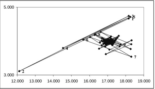
from the Italian stock market. In figures1 and 2we present the convergence behavior of a
pair of components of the vectorw, the same for all cases. We note that there is a significant
improvement in the convergence when we introduce the optimization of the weights with respect to the standard Ces`aro weights.
For more detailed results and computation time and for a comparisons with other
1 2 4 5 3 6 7 8 9 3.000 5.000 12.000 13.000 14.000 15.000 16.000 17.000 18.000 19.000
Figure 1: Example of convergence behavior for (wi, wj), two components of the vector w,
along the iterations with Ces`aro matrix.
1 2 3 4 56 7 8 9 3.000 5.000 12.000 13.000 14.000 15.000 16.000 17.000 18.000 19.000
Figure 2: Example of convergence behavior for (wi, wj), two components of the vector w,
6
Conclusion
We proposed a time and nodal decomposition approach to solve a wide class of multistage stochastic programming problems.
The method, starting from a multistage stochastic programming problem in arborescent formulation, reformulates the problem as a discrete time optimal control problem and applies a discrete version of Pontryagin’s maximum principle to obtain the necessary conditions for optimality.
These steps decompose the problem with respect to time and nodes obtaining small subproblems to be solved. To aggregate the solutions of the subproblems, which are optimal only with respect to each subproblem in each iteration, and to converge to the optimal solution of the original problem an iterative scheme is introduced. In this step it is important to improve the speed of convergence. To this aim we propose to introduce a further optimization step choosing in each iteration the optimal weights to combine solutions from previous iterations. This can be done in different ways, in this contribution we suggest two methods.
The results obtained for some test problems show that the proposed decomposition method with the further optimization step over the convex region obtained from previous iterations, can solve very large optimization problems reaching the optimal solutions in a very efficient way requiring a relative low computational time and a small number of iterations.
References
[1] Barro, D., Canestrelli, E.: Dynamic portfolio optimization: Time decomposition using
the Maximum principle with a scenario approach. European Journal of Operational
Research163 (2005) 217-229
[2] Barro, D., Canestrelli, E.: Time and nodal decomposition with implicit
non-anticipativity constraints in dynamic portfolio optimization. Mathematical Methods
in Economics and Finance 1 (2007) 1-24
[3] Barro, D., Canestrelli, E.: Tracking error: a multistage portfolio model. Annals of
Operations Research 165(1)(2009) 47-66.
[4] Birge, J.R.: Decomposition and partitioning methods for multistage stochastic
programs, Operation Research. 33(1985) 989-1007
[5] Birge, J.R., Louveaux, F.: Introduction to stochastic programming. Springer, New
York (1997)
[6] Canon, M.D., Cullum, C.D.Jr, Polak, E.: Theory of optimal control and mathematical
programming. McGraw Hill, New York (1970)
[7] Borwein, J., Reich S., Shafrir, I.: Krasnoleski-Mann iterations in normed spaces.
[8] Brezinski, C., Chehab J-P.: Nonlinear hybrid procedures and fixed point iterations.
Numerical Functional Analysis and Optimization 19(1998) 465-487
[9] Combettes, P.L., Pennanen T.: Generalized Mann iterates for constructing fixed points
in Hilbert spaces. Journal of Mathematical Analysis and Applications275(2002)
521-536
[10] Dupaˇcov´a, J., Consigli G., Wallace, S.W.: Scenarios for multistage stochastic
programming. Annals of Operations Research 100(2000) 25-53
[11] Dunn, J.C., Bertsekas, D.P.: Efficient dynamic programming implementations of
Newton’s method for unconstrained optimal control problems. Journal of Optimization
Theory and Applications 63(1989) 23-38
[12] Evtushenko, Y.G.: Numerical optimization techniques. Optimization Software Inc.,
New York (1985)
[13] Fisher, M.E., Jennings, L.S.: Discrete-time optimal control problems with general
constraints. ACM Transactions on Mathematical Software 18(1992) 401-413
[14] Franks, R.L., Marzec, R.P.: A theorem on mean-value iterations. Proceedings of the
American Mathematical Society30 (1971) 324-326
[15] Intriligator, M.D.: Mathematical optimization and economic theory. SIAM (2002)
[16] Mann, W.R.: Mean value methods in iteration. Proceedings of the American
Mathematical Society4 (1953) 506-510
[17] Mann, W.R.: Averaging to improve convergence of iterative processes. In Functional
Analysis Methods in Numerical Analysis, M. Zuhair Nashed ed., LNM vol. 701 Springer-Verlag, Berlin, (1979) 169-179
[18] Mulvey, J.M., Ruszczy´nski, A.: A digonal quadratic approximation method for large
scale linear programming. Operations Research Letters12 (1992) 205-215
[19] Ortega, A.J., Leake, R.S.: Discrete Maximum principle with state constrained control.
SIAM J. on Control and Optimization 15(1977) 119-147
[20] Polak, E.: Computational methods in optimization. Academic Press, New York (1971)
[21] Pytlak, R., Vinter, R.B.: Feasible direction algorithm for optimal control problems
with state and control constraints : Implementations. Journal of Optimization Theory
and Applications 101 (1999) 623-649
[22] Rhoades, B.E.: Fixed point iterations using infinite matrices. Transactions of the
American Mathematical Society196 (1974) 161-176
[23] Rockafellar, R.T.: Duality and optimality in multistage stochastic programming.
[24] Rockafellar, R.T., Wets, R.B.J.: Generalized linear quadratic problems of deterministic and stochastic optimal control in discrete time. SIAM J. on Control and Optimization
28 (1990) 810-822
[25] Rockafellar, R.T., Wets, R.B.J.: Scenario and policy aggregation in optimization under
uncertainty. Mathematics of Operations Research 16(1991) 119-147
[26] Rockafellar, R.T., Zhu, C.Y.: Primal-dual projected gradient algorithms for extended
linear quadratic programming. SIAM Journal on Optimization3 (1993) 751-783
[27] Rosa, C., Ruszczynski, A.: On Augmented Lagrangian decomposition methods for
multistage stochastic programs. Annals of Operations Research 64(1996) 289-309
[28] Ruszczynski, A.: A regularized decomposition for minimizing a sum of polyhedral
functions. Mathematical programming35 (1986) 309-333
[29] Ruszczynski, A.: An augmented lagrangian decomposition method for block diagonal
linear programming problems. Operations Research Letters8 (1989) 287-294
[30] Ruszczynski, A.: Parallel decomposition of multistage stochastic programming
problems. Mathematical programming 58(1993) 201-228
[31] Sethi, S.P., Thompson, G.L.: Optimal control theory: applications to management
science and economics. Kluwer Academic Publishers, Boston (2000)
[32] Schwarz, H.R.: Numerical analysis: a comprehensive introduction. John Wiley & Sons,
Chichester (1989)
[33] Van Slyke R., Wets R.B.J.: L-Shaped linear programs with applications to optimal
control and stochastic linear programs. SIAM J. Appl. Math. 17(1969) 638-663
[34] Wallace, S.W., Helgason, T.: Structural properties of the Progressive Hedging
Algorithm. Annals of Operations Research31 (1991) 445-456
[35] Wallace, S.W., Ziemba, W.T. (eds.): Applications of Stochastic Programming. SIAM
Mathematical Programming Series on Optimization, SIAM, Philadelphia (2005)
[36] Wright, S.J.: Interior point methods for optimal control of discrete time systems.
Journal of Optimization Theory and Applications 77(1993) 161-187
[37] W.T. Ziemba, J.M. Mulvey (eds.), World Wide Asset and Liability Modeling.