Towards data driven selection of a penalty function for data driven Neyman tests

(1)

www.elsevier.com/locate/laa

Towards data driven selection of a penalty function

for data driven Neyman tests

Tadeusz Inglot, Teresa Ledwina

∗

Institute of Mathematics, Polish Academy of Sciences, ul. Kopernika 18, 51-617 Wrocław, Poland

Received 20 December 2004; accepted 24 October 2005 Available online 15 December 2005

Submitted by A. Markiewicz

Abstract

The data driven Neyman statistic consists of two elements: a score statistic in a finite dimensional submodel and a selection rule to determine the best fitted submodel. For instance, Schwarz BIC and Akaike AIC rules are often applied in such constructions. For moderate sample sizes AIC is sensitive in detecting complex models, while BIC works well for relatively simple structures. When the sample size is moderate, the choice of selection rule for determining a best fitted model from a number of models has a substantial influence on the power of the related data driven Neyman test. This paper proposes a new solution, in which the type of penalty (AIC or BIC) is chosen on the basis of the data. The resulting refined data driven test combines the advantages of these two selection rules.

Keywords: Akaike criterion; Asymptotic optimality; Data driven test; Goodness of fit; Neyman test; Power comparison; Schwarz selection rule

1. Introduction

Data driven Neyman tests are based on two elements: Neyman’s smooth statistic (or equiva-lently, score statistic) in a finite dimensional submodel and a selection rule to choose the appro-priate submodel. Ledwina [20] introduced such a construction for the case of testing uniformity, proposing to use Schwarz [24] BIC criterion as the selection rule. There was clear motivation for such a choice. The smooth statistic can be naturally related to some testing problem in a

∗Corresponding author. Tel.: +48 71 372 8895; fax: +48 71 348 1098.

(2)

finite dimensional exponential family, while the Schwarz rule was simply designed to select the dimension of the exponential model. Obviously, some extensions of the original Schwarz rule were available at that time, allowing for a large range of penalties (cf. [9, Remark 1.2]). However, an appealing feature of Schwarz’s solution was the large penalty, which results in the selection rule behaving nicely for “small” models, using the handy formulation of Shen and Ye [25]. This guarantees that the construction of the related test is consistent with the following, often very natural, assumption. A researcher has some knowledge about the phenomenon under investigation and this is reflected by the form of the null model. Consequently, small, rather than large departures, from the null model are expected. This postulate is silently assumed in many simulation studies. For illustration, almost every alternative to normality listed in [22] can be considered as a small departure (as explained in Sections2 and5) from the null model. In contrast, large departures from normality could be defined by multimodal mixtures or heavy tailed distributions.

In recent years, many other penalized statistics with smaller penalties, such as Akaike [2] or modified forms of BIC, have been proposed. In particular, such an approach appeared in goodness-of-fit tests for some regression problems. See [1,7,8] for some examples and further references. Such a choice is motivated by the greater complexity of the underlying models and imprecise knowledge regarding the null and alternative distributions. It seems that the terminologylack of fit test, often used in the context of regression, instead ofgoodness of fit test, typically associated with fitting distributions, also reflects the greater uncertainty related to some regression problems. Since small penalties are associated with detecting “large” models, again using the terminology of Shen and Ye [25], the effect is that the related tests are less powerful for small departures (from the null hypothesis) than those related to BIC.

This paper aims to propose a solution that has the advantages of both types of penalty. For conciseness we restrict attention to testing uniformity and two (simplified) selection rules: BIC and AIC. Roughly speaking, the basic idea is, given the data, to decide which penalty should be used to select the number of terms in the score statistic. The new solution, together with some optimality properties, is described in Section2. Section3presents a simulation study showing the advantages of the refined version of the data driven test. Section4briefly discusses the asymptotic behaviour of new test statistic under the null hypothesis. In Section5some possible extensions are indicated.

2. The new test

We start with some notation and discussion. For brevity we only consider Neyman’s original test related to the Legendre system. Letb1, b2, . . .be orthonormal Legendre polynomials with

respect to Lebesgue measure defined on[0,1]. LetX1, . . . , Xnbe i.i.d. each distributed according

to a continuous distribution with densityp(x)with respect to Lebesgue measure on[0,1]. The null hypothesisH0asserts thatp=p0, wherep0(x)≡1 forx∈ [0,1]. Denote the distribution

corresponding top0byP0.

Consider the following probabilistic model for departures fromp0:

pk(x;θ )=p0(x)  ck(θ )exp    k j=1 θjbj(x)     , (1) whereθ =(θ1, . . . , θk) and ck(θ ) is the normalizing factor. Obviously, EP0bj(X1)=0 and EP0bi(X1)bj(X1)=δij, i, j =1,2, . . ., whereδij is the Kronecker delta.

(3)

The score statistic for testingθ1= · · · =θk=0 in (1) is of the form Nk= k j=1 {√nbˆj}2, where bˆj = 1 n n i=1 bj(Xi).

Obviously, the same score test would be obtained when considering any other type of departure with approximate structure 1+k_i₌₁θjbj(x)forθ1, . . . , θkclose to 0.

The simplified BIC and AIC are defined by

S1=min1kd(n):Nk−klognNj−jlogn, j =1, . . . , d(n)

and

A1=min1kd(n):Nk−2kNj−2j, j=1, . . . , d(n)

,

whered(n)is the number of models in the list. As seen, the simplification relies on replacing the maximized loglikelihood for (1) by(1/2)Nk, which is the standard approximation resulting

from the delta method. The original versions of AIC and BIC could be considered as well, with the outcome expected to be similar, but we prefer to consider the simplest set-up.A1 andS1 are examples of so called score-based selection rules, whileNA1andNS1are data driven Neyman’s

tests.

The asymptotic properties ofNS1were studied by Inglot [10] and Inglot and Ledwina [12]. In

these papers the notationS2 was used for the simplified Schwarz rule. Kallenberg [15] considered a large class of data driven tests corresponding to a variety of penalties, includingA1 andS1 as special cases. In particular, Kallenberg [15] proved that tests based onNA1andNS1are locally

optimal in the sense of vanishing shortcoming (cf. his Theorem 4.7 and the comment following it). However, local asymptotic optimality does not exclude the situation that for moderate sample sizes, fixed alternatives and significance levels, the powers ofNA1andNS1may be substantially

different. Some evidence is presented in Tables2–4of Section3. An explanation is given below. Note that, as typical for penalized criteria, in many cases the argument is understood in relation to the actual sample size.

Akaike’s small penalty results in the inconsistency of the criterion (cf. [27]) and, as a conse-quence, in large critical values (see Table1for illustration). Hence, for “small” models, such as those defined mainly by three or four not very large, low order Fourier coefficients,NA1is much

weaker thanNS1, as the critical value is overestimated in the context of real data (remember that Nkis the score statistic in (1)). On the other hand, Schwarz’s large penalty causes oversmoothing

for moderaten. Hence, the power ofNS1for models with relatively large higher order Fourier

coefficients is much smaller than that ofNA1, as large components are not included in the test

statistic for relatively smalln’s. However, a large penalty is profitable in the sense that the critical value is small in comparison to the critical value obtained using AIC. This enables attaining high power for models with relatively large low order Fourier coefficients. For illustration, see the casesj =1 andj =8 in Table2.

We propose to balance these two extreme tendencies as follows: useA1 only when an alternative is very distant from the null distribution, otherwise useS1. Using such an approach, the only missing element is an indication of how to decide whether we are close to the null model or not. To address this question, we propose to use the simple threshold rule described below.

Set In(c)=1 max 1jd(n)| √ nbˆj| clogn , (2)

(4)

where1(•)is the indicator of the set•. Observe that under the null hypothesis√nbˆ1, . . . ,

√ nbˆn

are uncorrelated and approximatelyN (0,1). Moreover, asymptotically they have i.i.d.N (0,1)

distributions. The thresholdclogn, c2, is an adaptation of the standard solution for a white noise sequence of independent and identically distributedN (0,1)variablesZ1, . . . , Znfor which

P r max 1jn|Zi|> 2 logn →0, asn→ ∞

(cf. [5, p. 445], for such a choice of threshold). Therefore, an intuitive conclusion is thatIn(c)=1

whenc≈2, c >2, indicates that the distribution of observations is close to the null model. Some simple, more formal, argument is provided inAppendix A. On the other hand, consider an alterna-tive distributionP, absolutely continuous with respect to Lebesgue measure, as assumed before. Then, there existsK=K(P ), such thatEPb1(X1)= · · · =EPbK−1(X1)=0 andEPbK(X1) /=

0, cf. [23, pp. 178, 191–192 withθ (x)=p(x)−1]. Simultaneously,max1jd(n)| √

nbˆj|

clogn⊃|√nbˆK|

clogn, provided thatd(n)K. Therefore, by WLLN, for any{d(n)}, such thatd(n)→ ∞asn→ ∞and any positivec, under any arbitrary alternativeP, it holds that

lim

n→∞P (In(c)=0)=1. (3)

In our simulation study we tookc=c0=2.4. For some explanation of this choice see Section

3.

Now define the new penalty by

π(j, n)= {jlogn}{In(c0)} + {2j}{1−In(c0)}, (4)

and the new selection rule by

T1=min1kd(n):Nk−π(k, n)Nj −π(j, n), j=1, . . . , d(n)

.

The new data driven statisticNT1is defined analogously toNS1andNA1.

SinceS1T1A1 holds forn8, one getsNS1NT1NA1. Therefore, local optimality

in the sense of vanishing shortcoming forNT1 can be established by exploiting some known

auxiliary results forNA1andNS1(see [15]). We shall not derive and formulate a precise result.

Instead, in the next section we present a fragment of a simulation study, we performed to investigate the power behaviour ofNT1for finite samples and to compare it with a recently introduced test

based on the likelihood ratio (see [28]).

3. The performance ofT1 andN_T1in the simulation study

Let us start with some comments on the choice ofcin the definition ofIn(c)(cf. (2)). Obviously,

the choice ofcis critical to the performance ofT1 andNT1, both under the null and alternative

hypotheses, when the sample size is moderate. Roughly speaking, under the alternative, the Schwarz rule is almost always selected for largec, while for smallcAkaike penalty is frequently preferred. There is also empirical evidence thatT1 andNT1change smoothly ascincreases. For

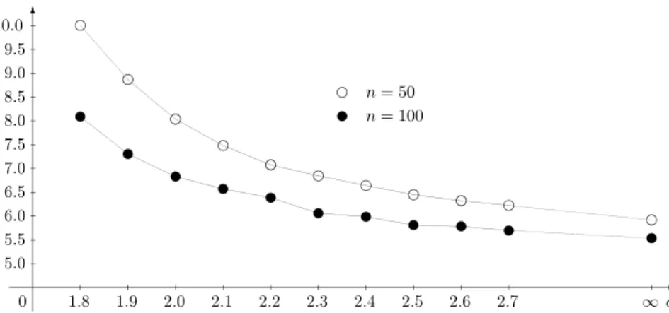
illustration see Figs.1and2. In Fig.2,c=0 corresponds to the application of AIC, whilec= ∞

means BIC was used.

Our choice of the regularization is subjective. We focused on a value of cthat allows AIC to act only if really large departures from the null model are present. Our optionc=c0=2.4

(5)

Fig. 1. The behaviour of simulated critical values ofNT1according to the switching constantc.n=100,α=0.05, 10,000 MC.

Fig. 2. The behaviour of simulated powers ofNT1according to the switching constantc.n=100,α=0.05, 10,000 MC.

results in power comparable to that ofNS1when we have ‘smooth’ disturbances of the null model

in the rough sense formulated by Neyman [21], i.e. when up to 3 or 4 of the initial components

{√nbˆj}2, j =1,2, . . .are significantly large. For illustration see Fig. 2 and Tables2–4. Our

choice also guarantees power comparable to that ofNS1if disturbances are small. On the other

hand, for alternatives very far from the null model, such as, e.g., highly oscillating alternatives, the new solution essentially inherits the properties ofNA1. Obviously, as in the case ofA1 and S1, when discussingT1 the complexity and size of the disturbances is understood relative to the sample size.

Throughout we considern=100, d(n)=12 and significance levelα=0.05. Each MC exper-iment was repeated 10,000 times.

Table1 presents critical values ofNA1, NS1 andNT1 and empirical behaviour of the three

selection rules when the null hypothesisH0is true. Note that in this experiment the number of

cases in whichT1=S1 was 9858.

We also present some empirical powers under three types of departures: gj(x;ρ)=1+ ρcos(j x), ρ ∈(0,1], j =1,2, . . . , pk(x;θ ), θ∈Rk, k=1,2, . . ., given by (1) and h(x;, p, q)=1−+βp,q(x),∈ [0,1], p, q >0, whereβp,q(x)stands for the beta density.

To have some insight into the structure and magnitude of the alternatives, in each case we calculated (using an MC method)d(n)=12 Fourier coefficients (in the Legendre basis) of the underlying

(6)

Table 1

Empirical behaviour ofNA1, NS1, NT1and selection rules under uniformity Statistic Critical Frequency in 10,000 simulations

value k 1 2 3 4 5 6 7 8 9 10 11 12 NA1 15.684 {A1=k} 7201 1086 549 353 211 163 131 93 86 77 50 0 NS1 5.527 {S1=k} 9613 323 47 14 1 1 0 0 1 0 0 0 NT1 5.987 {T1=k} 9536 295 57 25 13 17 13 13 11 12 8 0 n=100,d(n)=12,α=0.05, 10,000 MC runs. Table 2

Empirical powers of Zhang’s test and tests based onNA1, NS1andNT1under the alternativegj(x;ρ)

Parameters The five largest (in absolute value) Empirical powers Percentage

j ρ Fourier coefficients×1000 (as percentages) of cases

ZA NA1 NS1 NT1 T1=S1 1 0.45 [1]315 [3]39 [8]2 [12]1 [2]1 76 32 81 78 56 2 0.40 [2]273 [4]79 [6]6 [1]2 [8]2 18 34 70 68 71 3 0.50 [3]316 [5]149 [1]40 [7]23 [9]4 34 54 65 65 54 4 0.60 [4]335 [6]235 [2]102 [8]58 [10]8 17 86 64 71 37 5 0.70 [7]320 [5]317 [3]173 [9]108 [1]20 41 97 60 78 27 6 0.70 [8]347 [6]232 [4]209 [10]156 [2]53 14 98 46 77 27 7 0.75 [9]377 [5]238 [11]217 [7]147 [3]98 33 98 33 81 20 8 0.80 [10]385 [12]280 [6]245 [4]141 [8]50 13 99 34 90 11 n=100,d(n)=12,α=0.05, 10,000 MC runs.

distributions. The five largest (from these 12) Fourier coefficients are presented in Tables2–4. We also display the percentage of cases in whichT1=S1.

The results are encouraging. The new solution outperforms the power behaviour ofNA1for

smooth alternatives and is comparable toNS1in these cases. For highly oscillating alternativesNT1

is much more powerful thanNS1and not much less powerful thanNA1. Also,NT1outperforms

the power behaviour ofZA, recently introduced by Zhang [28], as an improved construction

compared to traditional tests. For many cases considered in Tables2–4, further comparisons with the powers of the solution proposed by Bickel and Ritov [3], the classical chi-square test, as well as many data driven versions of it, introduced and studied in [4], as well as in [11] are possible. Simulations for the test of Bickel and Ritov [3] can be found in [16]. Again, such inspection shows that the new test competes well with other procedures.

4. The limiting distribution ofN_T1under uniformity and consistency under alternatives

From (A.1) ofAppendix A, whenc2 andd(n)log3n/n→0 asn→ ∞, we haveP0(T1=/ S1)→0 asn→ ∞. SinceP0(S1=1)→1 (cf. [12, (2.4)], e.g., as mentioned earlierS1 isS2 in

that paper), we infer that the asymptotic null distribution ofNT1is chi-square with one degree of

freedom. The convergence is rather slow. For example, in Table1the simulated critical value of

NT1is 5.987, while the limiting value is 3.841. A similar phenomenon was observed in the cases

of the original and simplified Schwarz rules. Kallenberg and Ledwina [17] described a simple, nicely working approximation, which can serve to calculatep-values and which can be adopted to

(7)

Table 3

Empirical powers of Zhang’s test and tests based onNA1, NS1andNT1under the alternativepk(x;θ )

k θ Fourier coefficients×1000 (as percentages) of cases

ZA NA1 NS1 NT1 T1=S1 1 0.3 [1]295 [2]38 [9]2 [12]1 [11]1 70 28 74 71 64 2 (−0.2,−0.3) [2]256 [1]151 [3]40 [4]31 [5]5 70 24 75 73 79 3 (0,0,0.4) [3]395 [6]66 [2]47 [4]44 [5]14 53 69 87 87 26 4 (0,−0.3,0,−0.2) [2]223 [4]134 [6]42 [8]8 [10]2 66 14 52 48 89 4 (0.1,0.15,−0.25, [4]335 [3]235 [1]150 [2]137 [7]68 47 86 85 86 39 −0.35) 5 (0,0,0,0,0.4) [5]397 [10]67 [2]48 [8]41 [4]40 31 77 56 76 25 6 (0.1,0,0,0.1, [5]277 [6]272 [4]176 [1]165 [7]78 62 84 61 66 47 0.2,0.2) 8 (0,0,0,0,0,0,0, [8]450 [2]55 [4]36 [12]26 [6]21 7 93 30 90 9 −0.5) n=100,d(n)=12,α=0.05, 10,000 MC runs. Table 4

Empirical powers of Zhang’s test and tests based onNA1, NS1andNT1under the alternativeh(x;ε, p, q)

ε p q Fourier coefficients×1000 (as percentages) of cases

ZA NA1 NS1 NT1 T1=S1 1 1.5 1.5 [2]280 [4]46 [6]18 [8]8 [10]5 75 17 75 72 73 0.25 2.0 10.0 [1]289 [2]129 [4]116 [5]95 [6]49 63 47 76 73 64 0.25 10.0 20.0 [3]225 [2]161 [5]161 [1]143 [6]97 38 57 59 58 79 0.50 0.8 1.5 [1]263 [3]62 [2]59 [5]36 [4]34 66 28 64 61 74 0.50 0.8 0.5 [2]217 [1]199 [4]158 [3]144 [6]130 79 71 71 71 62 0.60 0.5 0.5 [2]334 [4]254 [6]211 [8]184 [10]166 89 86 88 88 33 0.20 0.2 0.2 [12]300 [10]296 [8]287 [6]281 [4]270 98 93 80 85 25 0.10 0.1 0.1 [12]273 [10]260 [8]244 [6]227 [4]201 97 84 58 68 40 n=100,d(n)=12,α=0.05, 10,000 MC runs.

the present situation. The main idea of this approximation is also given in [18], where an extension to the case in which some nuisance parameters are present is also shown.

From (3), under any alternative P we have P (T1=A1)→1 as n→ ∞. Therefore, the question of the consistency of NT1 is equivalent to establishing the consistency of NA1. This

problem was solved in [15], Section3.

5. Discussion

In this paper we have proposed a method of extending the sensitivity of data driven Neyman tests defined using a (simplified) Schwarz selection rule to determine the number of components. Though, for brevity, we restricted attention to testing uniformity, it is clear that the same idea can be applied to other problems where similar constructions have been proposed or to other new applications. For illustration, let us mention three cases in which score statistics along with (simplified) Schwarz selection rules have been successfully applied. Testing goodness-of-fit when

(8)

some Euclidean nuisance parameters are present and a score based-selection rule applied has been treated, e.g., in [19, see statistic (2.7) therein]. A nonparametric two-sample problem was considered in [14, see (14) there]. Semiparametric linear regression was studied in [13, cf. Section 3.4 of that paper]. To make some more precise remarks, let us consider the first problem and testing normality as a particular application. Since nuisance parameters are present, the score statistic is of the following form:

Wk(vˆ)=nVk(vˆ){Mk(vˆ)}VkT(vˆ),

wherev=(EX,VarX) is the vector of nuisance parameters,vˆ is an appropriate estimator of

v, whileVk(v)is efficient score vector.Mk(v)is the inverse of the covariance matrix ofVk(v).

T denotes transposition. For a location-scale family and appropriate estimators ofvthe matrix

Mk(v)is independent ofvand equalsMk, say. In particular, this is the case for testing normality

when MLEs are used. In such a case we have

Wk(vˆ)=nVk(vˆ){Mk}VTk(vˆ)= k

j=1

{√nUj(vˆ)}2,

whereUj(vˆ)is thejth component ofVk(vˆ)M1_k/2. Under the null model √

nU1(vˆ), . . . ,

√ nUk(vˆ)

are asymptotically i.i.d.N (0,1). The data driven score statistic is of the formW_S₁₍_v_ˆ₎(vˆ), where

S1(vˆ)is defined asS1 in Section2withWk(vˆ)in place ofNk; cf. also (2.6) in [19]. Therefore,

it is clear that√nUj(vˆ) can be used instead of √

nbˆj in (2), to obtain a refined version of W_S1(ˆv)(vˆ).

To get some intuition regarding the behaviour of Uj(vˆ), we inspected their (averaged over

10,000 MC runs) values in several cases taken from the extensive simulation study of Kallenberg and Ledwina [19]. This study covers, among others, alternatives from [22]. In all the cases we studied, exceptT U (0.7), we observed that the averagedUj(vˆ)’s follow the same pattern: the

componentj =2 orj =3 is dominant. ForT U (0.7)the dominant components are:j =6,4,8 (in order of their magnitude). However, the empirical power whenn=100 and α=0.05 is 0.90 in this case. So, there is no room for much improvement for samples of that size or larger.

T U (0.7)is an example of a distribution with a heavier tail than the normal distribution. Higher order components are also dominant in cases of multimodal normal mixtures, for example. So, this class of departures leaves room for some improvement.

Anyway, it is clear that the construction applies to more complex situations as well, where some less regular disturbances may be expected. For example, Fan [6] constructed a two-sample test focused on detecting local characters such as sharp peaks. Guerre and Lavergne [7] proposed a test for regression, which is powerful in detecting highly oscillating alternatives. The refined method proposed in this paper allows us to construct more universal solutions in such cases. Such an application has been recently successfully introduced in [13]. For a practical compari-son of Fan’s test to related data driven tests with a score-based selection rule incorporated, see [14].

Acknowledgments

We are grateful to a reviewer for helpful comments. The programming work was done by A. Janic-Wróblewska. Her kind co-operation is gratefully acknowledged. The research was supported by Polish State Committee of Scientific Research Grant 5 P03A 03020.

(9)

Appendix A

Consider the event

An(c)= max 1jd(n)| √ nbˆj|> clogn

and assume throughout thatc2 andd(n)log3n/n→0 asn→ ∞. Since|bj(x)|√2j+1, x ∈ [0,1], from Bernstein’s inequality (cf. [26, p. 855]) applied withϑj =1, K=√2j +1 and λ=clogn, we get P0(An(c)) d(n) j=1 P0 |√nbˆj| clogn 2 d(n) j=1 exp −1 2 · clogn {1+(1/3)(2j +1)(clogn)/n} .

Hence, by the assumptiond(n)log3n/n→0, we obtain for largenand some positive constant

C P0(An(c)){C}{d(n)}/{n1+}, = _c 2 −1 . (A.1)

(A.1) implies that limn→∞P0(T1=S1)=1.

Assuming additionally thatc >2,d(n)=O(nγ), γ =γ (c) < , we get∞_n₌1P0(An(c)) < ∞. Therefore, in this case the Borel–Cantelli lemma yields

P0 max 1jd(n)| √ nbˆj|>

clogninfinitely often

=0. (A.2)

This shows that whenc >2,In(c)=0 is highly unprobable underH0for largen. Whenc 2,

(A.2) implies a lot of room for some shift in the means ofbˆj’s. Therefore, the resultIn(c)=0

indicates that observations come from some distribution significantly different fromP0. References

[1] M. Aerts, G. Claeskens, J.D. Hart, Testing lack of fit in multiple regression, Biomertika 87 (2000) 405–424. [2] H. Akaike, A new look at statistical model identification, IEEE Trans. Automat. Control 19 (1974) 716–723. [3] P.J. Bickel, Y. Ritov, Testing for goodness of fit: a new approach, in: A. Saleh (Ed.), Nonparametric Statistics and

Related Topics, Amsterdam, North-Holland, 1992, pp. 51–57.

[4] M. Bogdan, Data driven versions of Pearson’s chi-square test for uniformity, J. Statist. Comput. Simulation 52 (1995) 217–237.

[5] D.L. Donoho, I.M. Johnstone, Ideal spatial adaptation by wavelet shrinkage, Biometrika 81 (1994) 425–455. [6] J. Fan, Test of significance based on wavelet thresholding and Neyman’s truncation, J. Amer. Statist. Assoc. 91

(1996) 674–688.

[7] E. Guerre, P. Lavergne, Data-driven rate optimal specification testing in regression models, Ann. Statist. 33 (2005) 840–870.

[8] E.J. Hannan, B.G. Quinn, The determination of the order of autoregression, J. Roy. Statist. Soc., Ser. B 41 (1979) 190–195.

[9] D.M.A. Haughton, On the choice of a model to fit data from an exponential family, Ann. Statist. 16 (1988) 342–355. [10] T. Inglot, Generalized intermediate efficiency of goodness-of-fit tests, Math. Methods Statist. 8 (1999) 487–509. [11] T. Inglot, A. Janic-Wróblewska, Data driven chi-square test for uniformity with unequal cells, J. Statist. Comput.

(10)

[12] T. Inglot, T. Ledwina, Intermediate approach to comparison of some goodness-of-fit tests, Ann. Inst. Statist. Math. 53 (2001) 810–834.

[13] T. Inglot, T. Ledwina, Data driven score tests of fit for semiparametric homoscedstic linear regression model, submitted for publication.

[14] A. Janic-Wróblewska, T. Ledwina, Data driven-rank test for two-sample problem, Scand. J. Statist. 27 (2000) 281–297.

[15] W.C.M. Kallenberg, The penalty in data driven Neyman’s tests, Math. Methods Statist. 11 (2002) 323–340. [16] W.C.M. Kallenberg, T. Ledwina, Consistency and Monte Carlo simulation of a data driven version of smooth

goodness-of-fit tests, Ann. Statist. 23 (1995) 1594–1608.

[17] W.C.M. Kallenberg, T. Ledwina, On data driven Neyman’s tests, Probab. Math. Statist. 15 (1995) 409–426. [18] W.C.M. Kallenberg, T. Ledwina, Data-driven smooth tests when the hypothesis is composite, J. Amer. Statist. Assoc.

92 (1997) 1094–1104.

[19] W.C.M. Kallenberg, T. Ledwina, Data driven smooth tests for composite hypotheses: Comparison of powers, J. Statist. Comput. Simulation 59 (1997) 101–121.

[20] T. Ledwina, Data-driven version of Neyman’s smooth test of fit, J. Amer. Statist. Assoc. 89 (1994) 1000–1005. [21] J. Neyman, ‘Smooth test’ for goodness of fit, Skand. Aktuarietidskr. 20 (1937) 159–199.

[22] E.S. Pearson, R.B. D’Agostino, K.O. Bowman, Tests for departures from normality: comparison of powers, Biometrika 64 (1977) 231–246.

[23] G. Sansone, Orthogonal Functions, Interscience, New York, 1959.

[24] G. Schwarz, Estimating the dimension of a model, Ann. Statist. 6 (1978) 461–464. [25] X. Shen, J. Ye, Adaptive model selection, J. Amer. Statist. Assoc. 97 (2002) 210–221.

[26] G. Shorack, J.A. Wellner, Empirical Processes with Application to Statistics, Wiley, New York, 1986. [27] M. Woodroofe, On model selection and the arc sin laws, Ann. Statist. 10 (1982) 1182–1194.