This thesis must be used in accordance with the
provisions of the Copyright Act 1968.
Reproduction of material protected by copyright
may be an infringement of copyright and
copyright owners may be entitled to take
legal action against persons who infringe their
copyright.
Section 51 (2) of the Copyright Act permits
an authorized officer of a university library or
archives to provide a copy (by communication
or otherwise) of an unpublished thesis kept in
the library or archives, to a person who satisfies
the authorized officer that he or she requires
the reproduction for the purposes of research
or study.
The Copyright Act grants the creator of a work
a number of moral rights, specifically the right of
attribution, the right against false attribution and
the right of integrity.
You may infringe the author’s moral rights if you:
- fail to acknowledge the author of this thesis if
you quote sections from the work
- attribute this thesis to another author
- subject this thesis to derogatory treatment
which may prejudice the author’s reputation
For further information contact the University’s
Director of Copyright Services
Rolling Window Time Series Prediction
using MapReduce
Author: Lei Li
Supervisor: Prof Philip Leong
A thesis submitted in fulfilment of the requirements for the degree of Master of Philosophy
in the
School of Electrical and Information Engineering at the University of Sydney
I, LEI LI, declare that this thesis titled, “Rolling Window Time Series Prediction using MapReduce” and the work presented in it are my own. I confirm that:
This work was done wholly or mainly while in candidature for a research degree at University of Sydney.
Where any part of this thesis has previously been submitted for a degree or any other qualification at this University or any other institution, this has been clearly stated.
Where I have consulted the published work of others, this is always clearly at-tributed.
Where I have quoted from the work of others, the source is always given. With the exception of such quotations, this thesis is entirely my own work.
I have acknowledged all main sources of help.
Where the thesis is based on work done by myself jointly with others, I have made clear exactly what was done by others and what I have contributed myself.
Signed:
Date:
Abstract
Faculty of Engineering
School of Electrical and Information Engineering
Master of Philosophy
Rolling Window Time Series Prediction Using MapReduce
by LeiLI
Prediction of time series data is an important application in many domains. Despite their inherent advantages, traditional databases and MapReduce methodology are not ideally suited for this type of processing due to dependencies introduced by the sequen-tial nature of time series. In this thesis a novel framework is presented to facilitate retrieval and rolling window prediction of irregularly sampled large-scale time series data. By introducing a new index pool data structure, processing of time series can be efficiently parallelised. The proposed framework is implemented in R programming environment and utilises Hadoop to support parallelisation and fault tolerance. A sys-tematic multi-predictor selection model is designed and applied, in order to choose the best-fit algorithm for different circumstances. Additionally, the boosting method is de-ployed as a post-processing to further optimise the predictive results. Experimental results on a cloud-based platform indicate that the proposed framework scales linearly up to 32-nodes, and performs efficiently with a relatively optimised prediction.
First and foremost, I would like to express my gratitude to my supervisor, Prof. Philip Leong for his guidance, inspiring ideas, encouragement, precious time in reviewing my work and always expecting high standards.
I am thankful to Dr. Richard Davis for his valuable comments and discussions, as well as for reviewing my manuscripts which helped me to produce a well organised thesis. I am extremely grateful to my colleagues Farzad Noorian and Duncan Moss for their generous supports which helped me to complete this work in a timely manner.
Finally I would like thank my parents and Bo Gao for their love and care.
Declaration of Authorship i
Abstract iii
Acknowledgements iv
Contents v
List of Figures viii
List of Tables ix
1 Introduction 1
1.1 Motivation and Aims . . . 1
1.2 Assumptions . . . 3
1.3 Contribution . . . 3
1.4 Thesis Structure . . . 4
2 Background 5 2.1 Time Series Prediction . . . 6
2.1.1 Time Series . . . 6
2.1.2 Time Series Prediction . . . 7
2.1.3 Rolling Time Series Processing . . . 9
2.2 Parallel Computing . . . 10
2.2.1 Parallel in Financial Applications. . . 10
2.3 MapReduce . . . 10
2.3.1 Hadoop . . . 12
2.3.2 Hadoop Distribution File System . . . 13
2.3.3 HBase . . . 14
2.3.4 Rhipe Package . . . 14
2.4 Amazon Web Service . . . 15
2.4.1 Elastic Cloud Computing . . . 15
2.4.2 StarCluster . . . 16
2.5 Boosting . . . 17
2.6 Related Work . . . 18
3 Rolling window time series prediction using MapReduce 19
3.1 Issue of Rolling Analysis using Hadoop . . . 19
3.2 Proposed Methodology . . . 20
3.3 Design . . . 23
3.3.1 Data Storage and Index Pool . . . 23
3.3.2 Preprocessing . . . 24 3.3.3 Rolling Windows . . . 24 3.3.4 Prediction . . . 25 3.3.5 Finalisation . . . 25 3.4 Forecasting . . . 26 3.4.1 Multi-Predictor Model . . . 26
3.4.2 Linear Autoregressive Models . . . 27
3.4.2.1 AR model . . . 27
3.4.2.2 ARIMA models . . . 27
3.4.3 NARX Forecasting . . . 28
3.4.3.1 ETS . . . 28
3.4.3.2 SVM . . . 28
3.4.3.3 Artificial Neural Networks . . . 29
3.5 Summary . . . 30
4 Cloud-based Platform 32 4.1 Cloud Platform . . . 32
4.1.1 Comparison of Different Cloud Platform . . . 33
4.2 AWS . . . 34
4.2.1 Elastic Compute Cloud . . . 34
4.2.2 Instance Types . . . 35
4.2.3 Break-even Analysis of Instances . . . 36
4.2.4 StarCluster . . . 36 4.3 Rhipe Package . . . 38 4.3.1 Advantages of Rhipe . . . 39 4.3.2 Example. . . 40 4.3.2.1 Specification of Rhipe . . . 40 4.3.2.2 Visualisation of Rhipe . . . 42 4.4 Summary . . . 43 5 Boosting 46 5.1 Boosting . . . 46 5.1.1 Ensemble Schemes . . . 47
5.1.2 Gradient Boosting Machine . . . 47
5.1.3 Discussion about Boosting Algorithms . . . 49
5.1.3.1 How to Choose Weak Learners . . . 50
5.1.3.2 Boosting Implementation Issues . . . 50
5.2 Gbm Package . . . 51
5.2.1 Improving Boosting Methods . . . 51
5.2.1.1 Decreasing Learning Rate . . . 51
5.2.1.2 ANOVA Decomposition . . . 52
5.2.2 Loss Function. . . 52 5.2.3 Implementgbm Boosting . . . 53 5.2.4 Example. . . 53 5.3 Summary . . . 54 6 Results 55 6.1 Experiment Setup . . . 55 6.1.1 Experiment Environment . . . 55 6.1.2 Test Data . . . 55
6.1.3 Preprocessing and Window Size. . . 56
6.1.4 Preprocessing Steps . . . 56
6.2 Performance and Architecture Test . . . 57
6.2.1 Scaling Test . . . 57
6.2.2 Cost Estimation . . . 57
6.2.3 Multi Predictor Model Test . . . 59
6.2.4 Data Split Handling Comparison . . . 60
6.3 Boosting Result Comparison . . . 60
6.3.1 HitRate . . . 61
6.3.2 Boosting Sample . . . 61
6.3.3 Boosting Test . . . 62
6.3.4 Measuring Effectiveness of Learner Combinations . . . 64
6.4 Summary . . . 65 7 Conclusion 66 7.1 Summary . . . 66 7.2 Further Directions . . . 67 A Boosting Example 68 A.1 AdaBoost . . . 68
A.1.1 AdaBoost Algorithm . . . 68
A.2 Training and Weighting of Boosting . . . 69
A.3 Distribution Models ofgbm . . . 70
A.3.1 Gaussian . . . 70
A.3.2 AdaBoost . . . 70
A.3.3 Bernoulli . . . 70
A.3.4 Laplace . . . 71
A.3.5 Quantile regression . . . 71
A.3.6 Cox Proportional Hazard . . . 71
A.3.7 Poisson . . . 72
A.4 Boosting Example . . . 72
Bibliography 74
1.1 Issue of partial windows: a rolling window needs data from both windows
at split boundaries. . . 2
2.1 Overview of a cloud-based prediction system . . . 5
2.2 An example of a spot price time series plot . . . 6
2.3 Components of time series dataset . . . 7
2.4 Time series prediction using ARIMA model . . . 8
2.5 Overview of parallel processing within a MapReduce environment. . . 10
2.6 Overview of a multi-node Hadoop cluster. . . 13
3.1 The system’s architecture . . . 22
3.2 Flow of data in the proposed framework.. . . 23
3.3 The back-propagation neural network structure . . . 30
4.1 Break-even plot of AWS Reserved instances and On-Demand instance . . 37
4.2 The D & R computational framework. . . 39
4.3 Rhipe processing example . . . 43
4.4 Example of local Hadoop job . . . 43
4.5 Details of JobTracker. . . 44
4.6 Completion of map and reduce jobs. . . 44
6.1 Speedup of execution time versus cluster size . . . 58
3.1 Example of an index pool . . . 23
4.1 Price comparison of Amazon and Microsoft . . . 34
4.2 Service comparison of Amazon and Microsoft . . . 34
4.3 Fees comparison between Reserved and On-Demand instances . . . 36
4.4 Prices for light, medium and heavy Reserved instance . . . 37
4.5 Advantages of Rhipe . . . 39
6.1 AWS EC2 execution times for scaling test . . . 57
6.2 Cost estimation . . . 58
6.3 Performance comparison of different predictor model on a 16 node cluster. 59 6.4 Computational efficiency of the proposed architecture. . . 60
6.5 Boosting results for client volume prediction . . . 62
6.6 Boosting prediction results in four different foreign currencies . . . 63
6.7 Boosting results of different combination of models . . . 64
Introduction
1.1
Motivation and Aims
A time series is a record of variables across time, usually measured at equally spaced time intervals. Time series analysis forms the basis for a wide range of applications including physics, climate research, physiology, medical diagnostics, computational finance and economics [1,2]. Prediction, in particular, is an important aspect of time series analysis. It can be thought of as a form of data mining, namely forecasting future values based on the analysis of data’s historical behaviours.
Historically time series prediction was performed by statistician and analysts. With rapid growth in the number and size of time series, manual inspection of time series has become time-consuming, cumbersome and costly, creating a demand for an automatic system to forecast large number of univariate time series. For example, it is common to have over one thousand product lines that need forecasting at least monthly in a businesses. One of the recent attempts to address this need is the forecast package by Hyndman et al. [3]. It includes variants of the most popular automatic forecasting algorithms, most of which are based on as either exponential smoothing or autoregressive integrated moving average (ARIMA) models [4]. This thesis was initially motivated to improve the speed of forecasting using this package. It must be also noted that this package is implemented in R [5], a free software programming language for statistical computing analysis which has become the de facto tool in machine learning and time series analysis.
The past decade has seen tremendous advances in application of parallel computing to various fields. New principles and standards are being created to address different requirements, and algorithms undergo many changes to become scalable. This requires
Split 1 Split 2 Partial Windows Window 1 Window 4-2 Window 4-1 Window 2 Window 3 Window 3-2 Window 4 Window 5 Window 3-1
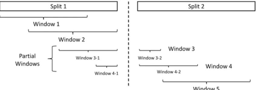
Figure 1.1: Issue of partial windows: a rolling window needs data from both windows at split boundaries.
not only an understanding of these algorithms, but of principles and techniques for parallel programming.
To achieve an efficient approach for analysing time series data in a parallel architecture, Hadoop is currently considered as the most appropriate option to try. Apache Hadoop, originally derived from the work of Google’s MapReduce [6], has become the standard way to address Big Data problems. MapReduce is used to process files on each node simultaneously and then aggregate their outputs to generate the final result. Hadoop allows for more scalable, cost effective, flexible and fault tolerant parallel programming [7].
Despite all of its advantages, the original MapReduce methodology of Hadoop is not ideally suited for time series analysis. This is due to the implicit dependencies among time series data observations [8]. Therefore partitioning and processing of time series data using Hadoop require additional considerations:
• Time series prediction algorithms operate on rolling windows, where a window of consecutive observations is used to predict the future samples. This fixed length window moves from the beginning of the data to the end of it. But in Hadoop, when the rolling window straddles two files, data from both are required to form a window and hence make a prediction (see Figure1.1).
• File sizes can vary depending on the number of time samples in each file.
• The best algorithm for performing prediction depends on the data and a consid-erable amount of expertise is required to design and configure a good predictor.
In addition, the issue of predictor algorithm selection and optimisation is critical, as is the implementation of an efficient platform that scales with time series data size. The main aim of this thesis is to develop a novel framework that can achieve parallel rolling time series prediction using Hadoop. By implementing the proposed framework, the system should be able to deal with massive amount of time series data, either regular
or irregular. Furthermore, the proposed system can handle the optimisation, parameter selection and also model combination through boosting.
1.2
Assumptions
In order to clarify the objectives of the thesis, certain assumptions are made in advance to give a better idea of what the proposed system is going to do and why it is significantly important to the time series prediction:
• The time series data is sufficiently large such that distributed processing is required to produce results in a timely manner.
• Time series prediction algorithms have high computational complexity so that an efficient and fast prediction model is urgently needed.
• Disk space concerns preclude making multiple copies of the data.
• The time series are organised in multiple files, where the file name is used to specify an ordering of its data. For example, daily data might be arranged with the date as its file name.
• In general, the data consists of vectors of fixed dimension which can be irregularly spaced in time.
1.3
Contribution
The first contribution of this thesis is a framework for rolling time series analysis using Hadoop [9]. The notion of a new index pool data structure is introduced, which is piv-otal for the entire framework to successfully solve the issues of dispatching regularly or irregularly sampled time series data to each computational node. The problems associ-ated with locating the index of time series data, architecture design issues, framework efficiency and flexibility are studied in detail. An efficient architecture is designed which enables the elegant handling of rolling time series forecasting smoothly, by using the MapReduce programming model.
Within the framework, a systematic approach to time series prediction is developed which facilitates the implementation and comparison of time series prediction algorithms in a wrapper model. A user-customisable multi-predictor model (MPM) is comprised of commonly used predictor algorithms. Applying the MPM in the proposed framework
not only allows algorithm auto-selection for a range of different circumstances, but also avoids common pitfalls such as over-fitting and peeking of data.
The third contribution is a feasibility study of deploying the proposed parallel rolling time series prediction system on a cloud-based platform. Considering its scalable pro-cessing capacity, cloud computing is a good alternative for performing big data analysis. Furthermore, the MapReduce model is in a suitable form for the applications deployed across cloud clusters. The further evaluation on the architecture performance and en-hancement of the scalability are achieved by implementing the proposed framework on Amazon Web Service (AWS) cloud clusters.
The last contribution is a study of applying boosting techniques to the proposed frame-work for a further prediction optimisation. A rolling procedure is employed within the boosting experiments to enhance the stability and predictive accuracy.
1.4
Thesis Structure
The remainder of the thesis is organised as follows. Chapter 2gives an introduction to relevant background on time series prediction, MapReduce, Amazon Web Service, boost-ing and reviews the related work in this field. Chapter3proposes the core methodology of using MapReduce to achieve rolling window prediction and the notion of a new data storage indexing design. Chapter 4compares two popular cloud services and has a fur-ther study on AWS cloud service. This chapter also describes the details about how Rhipe package performs in parallel processing. The following Chapter 5 contains the details on the ensemble scheme theory of boosting and gradient boosting machine. The descriptive parameter specification and implementation of thegbm package are included in the same chapter. Chapter6 presents the experimental results with rigorous analysis and discussion. Finally, the research conclusions are summarised and future research directions are outlined in Chapter 7. Some less important details about boosting tech-niques are included in AppendixA.
Background
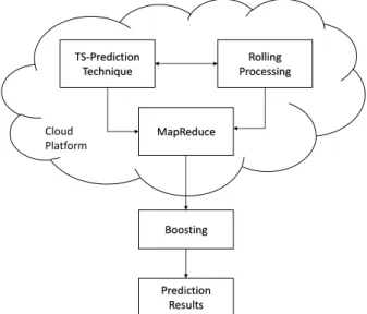
This chapter establishes the theoretical foundations on which the research in this thesis is based. Specifically, the areas covered are: time series prediction and techniques, rolling time series processing, MapReduce, Amazon Cloud Service and boosting techniques. The work presented in this thesis is an amalgamation of these research fields (see Figure2.1).
TS-Prediction Technique Rolling Processing Boosting Prediction Results MapReduce Cloud Platform
Figure 2.1: Overview of a cloud-based prediction system
Jul 01 00:00 Jul 08 00:00 Jul 15 00:00 Jul 22 00:00 Jul 29 00:00 0.00 0.05 0.10 0.15 0.20
Spot Price
Figure 2.2: An example of a spot price time series plot
2.1
Time Series Prediction
2.1.1 Time Series
A time series is defined as a sequence of data points observed typically at successive intervals in time [8]. It can be expressed as an ordered list: Y =y1, y2, . . . , yn [10]. Time series data is extensively used in many disciplines including statistics analysing, signal processing, weather forecasting, biology, mathematical economics and business management [2,11,12].
Figure2.2illustrates a spot price time series plot. The data are hourly aggregated spot prices of a small Linux AWS EC2 instance in the US east region for the one month period of July 2013. Notice that the data points have been connected through smoothing lines, which make it easier to follow the ups and downs over the time. The spot price for this particular EC2 instance fluctuates randomly.
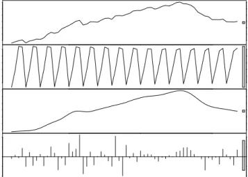
Many time series can be decomposed into four different components: the long term trend, seasonal components, irregular cycles, and random fluctuations [13]. In Figure2.3, the time series data are analytically decomposed into components, which are the quarterly retail trade index of 17 European countries from 1996 to 2011. In time series, adjacent observations are in a natural temporal ordering. This intrinsic feature of the time series makes its analysis dependent on the order of the observations, and distinct from other common data, in which there are no dependencies of the observations, such as contextual data [8].
90 96 102 data −0.3 0.0 seasonal 90 96 102 trend −0.4 0.2 2000 2005 2010 remainder time
Figure 2.3: Components of time series dataset
Time series analysis is defined as the methods for analysing the characteristics of time series data and extracting meaningful statistical information [14]. Time series forecast-ing is an important part of time series analysis, in which a model is used to predict future values based on previously observed values [15].
2.1.2 Time Series Prediction
Time series prediction is the use of past and current observations at timet to forecast future values at time t+l, where lis the horizon of prediction [8].
Linear time series models are well explored, with auto-regressive (AR) and moving aver-age (MA) models being central to modern stationary time series analysis. Hyndman and Khandakar developed a R library, namedforecast, for automatic time series forecasting [3]. In this package, some of popular forecasting algorithms are introduced which are principally based on exponential smoothing and autoregressive integrated moving aver-age (ARIMA) models. The automatic forecasting algorithms of the forecast select the appropriate time series model, estimate its parameters and then use it to predict the future values. [3]. Furthermore the forecast package contains robust algorithms that automatically deal with time series seasonal patterns and random fluctuations.
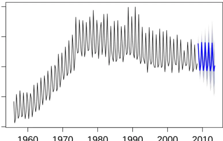
Figure 2.4 shows an example of a time series prediction using an ARIMA model. The example shows the quarterly beer production in Australia from 1958 Q1 to 2008 Q3, with the prediction objective of the next 20 quarters’ production using an ARIMA(1,1,2) model. The details of an ARIMA model are defined in Section 3.4.2.2.
Prediction
Years Production 1960 1970 1980 1990 2000 2010 200 300 400 500 600Figure 2.4: Time series prediction using ARIMA model
As the non-linear and non-stationary components often exist in real world time se-ries [16], non-linear approaches such as non-linear autoregressive processes, bilinear models and threshold models are developed and widely used for time series modelling. The generalised autoregressive conditional heteroskedasticity (GARCH) model is a non-linear time series model used to represent the changes of variance over time (het-eroskedasticity) [17], which is an extension of autoregressive conditional heteroskedasti-cicy (ARCH) [18]. ARCH and GARCH are used for the volatility of time series data in financial applications, but not studied in this thesis.
Financial time series prediction, however, is a special case as it is statistically different from other time series analysis. Its empirical time series usually contain a high degree of unpredictability, due to the existence of uncontrollable factors and potential or hidden risks influencing the financial markets. For example, the price of a fluctuating stock, which are truly random and not directly predictable, can be modeled as random walks. The theory of random walk states that, in a stock market, using the past observations of a stock price cannot predict its future movement [19, 20]. In the efficient market hypothesis (EMH), it is stated that market efficiency also has some reflections about the uncertainty of the future [21,22].
In this thesis we use three pure time-series models, namely ARIMA, naive and exponen-tial smoothing state space model (ETS), for the purposes of comparison. The drawback of model based approaches is that usually a priori assumption of the underlying distri-bution of data is required for model parameter estimation. Machine learning techniques
can alleviate this issue and cope with the inherent non-linear and non-stationary nature of real world time series.
2.1.3 Rolling Time Series Processing
Different dynamic and statistical methods are available for time series prediction [11]. Commonly, time series prediction algorithms operate on arolling window scheme. Let
{yi}, i = 1, . . . , N be a sampled, discrete time series of length N. For a given integer window size 0 < W ≤ N and all indices W ≤ k ≤ N, the h-step, h > 0, rolling (or sliding) window predictions,{yˆk+h} are computed:
ˆ
yk+h =f(yk−W+1, . . . , yk) (2.1)
where f is a prediction algorithm. ˆyk+h is approximated such that its error relative to
yk+h is minimised.
Rolling analysis of time series is usually applied to dynamically update the parameters of a model. A common technique is to compute parameter estimates through a fixed length rolling window of sample data. The estimates over the rolling windows should not be too different if the data are stationary. On the other hand, if the parameters change at some point during the sample, the rolling analysis should capture the changes on instability over the estimations [23]. Rolling analysis is often used for the backtesting of the historical time series data, so as to evaluate the stability of forecasting methods and improve the overall prediction accuracy [24]. The first step is to split the initial historical data into two parts, the estimation sample and the other sample for predic-tion. Then a statistical model is fitted into the estimation sample to forecast a k-steps ahead prediction for the prediction sample. The error measures can be deployed for calculating the difference between k-step ahead prediction and the observed prediction sample of historical data. By repeating the last two steps, the estimation sample is then rolled ahead with certain give rolling window length until it reach the end of historical estimation data sample. In the last step, all the predictive results of each single window are then summarised to calculate more statistics, such as the overall k-steps prediction errors, to evaluate the adequacy of the selected model. The rolling analysis often use moving average methods to conduct and evaluate the technical analysis of financial time series [24].
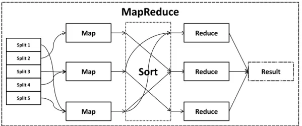
MapReduce
Sort
Map Map Map Split 1 Split 2 Split 3 Split 4 Split 5 Reduce Reduce Reduce ResultFigure 2.5: Overview of parallel processing within a MapReduce environment.
2.2
Parallel Computing
Parallel computing is defined as the simultaneous use of multiple computing resources to solve a computational problem [25]. The precondition of parallelism is that the problem is able to be broken apart into small parts and be processed simultaneously. The execution time with multiple computing processors is always expected less than with a single central processor. Parallel computing has been applied in various areas to improve the computation speed, such as data mining, signal processing and and computational simulation ranging from science to financial market [25].
2.2.1 Parallel in Financial Applications
With the increasing scale of stored transaction data in financial area, there are more and more concerns about parallel computing for financial analysis, in order to optimise business and marketing decisions. Many applications of quantitative finance are able to be parallelised, such as hedging, risk management and portfolio optimization. There-fore, the effective parallel computing modelling and methods are required urgently for financial time series analysis, in order to be competitive in the speed scaling [25]. Cur-rently MapReduce is one of the popular parallel computing mode for large-scale data computation.
2.3
MapReduce
The MapReduce programming model in its current form was proposed by Dean [26]. It centres around two functions, Map and Reduce, as illustrated in Figure 2.5. The first of these functions, Map, takes an input key-value pair, performs computations and
produces a list of key/value pairs as output, which can be expressed as (k1, v1) →
list(k2, v2). The Reduce function, expressed as (k2, list(v2)) → list(v3), takes all of the values associated with a particular key and applies computations to produce the results. Both Map and Reduce functions are designed to run concurrently and without any dependencies. To ensure that each Reduce receives the correct key, an intermediate sort step is introduced. Sort takes the list(k2, v2) and distributes the keys to the ap-propriate Reducers. The name MapReduce originally referred to the proprietary Google technology but has since become a generic term to describe this form of processing. The word count problem is often taken as the classic example to explain how MapReduce solves the real-world problem. The context is associated to the issue of counting the number of occurrences of particular words in a dictionary or big document [26]. The pseudocode designed in MapReduce model is listed below:
map(String key, String value) // key: document name
// value: document contents for each word w in value
EmitIntermediate(w, "1")
reduce(String key, Iterator values): // key: word
// values: a list of counts for each v in values:
result += ParseInt(v); Emit(AsString(result));
Themapis responsible for adding 1 to the count of occurrences where each word appears; The reduce function sums up all the counts for each single word.
The implementation of programming model MapReduce is an effective approach for processing large-scale data with a algorithm distributed in a parallel machine cluster. For example, using MapReduce to count student names in parallel: the Map procedure is responsible for sorting students by first name, and store each student name into queues. In the Reduce procedure, the counting number of students’ name and the frequency of each name is summarised. The MapReduce programming model can also be called infrastructure or framework. It benefits the parallelism of applications and computing tasks. By using MapReduce, all the data transfers and interaction between each single part of the system is becoming manageable, and also data redundancy and fault tolerance are considered.
The concept of MapReduce is inspired by the map and reduce functions in functional programming [26]. However, it has evolved and extended from their original forms and now has more powerful functionalities. The Map and Reduce functions are not the only major contribution, scalability and fault-tolerance are key to solving large-scale problems on commodity computing equipment [26]. The implementation of MapReduce in a single node or thread is not going to be faster than a traditional sequential computing. Only deploying MapReduce on a large cluster becomes beneficial for the optimisation of distributed operation, reduction on network communication cost and fault tolerance. Currently, MapReduce concepts have been applied in many areas and its libraries have been ported to various programming languages. The Apache Hadoop is one of the most popular implementations.
2.3.1 Hadoop
Apache Hadoop [27] is an implementation of the MapReduce framework for cluster computers constructed from computing nodes connected by a network, and was created by Doug Cutting and Mike Cafarella in 2005. It operates under the Java Runtime Environment (JRE) which ensures portability across platforms [28].
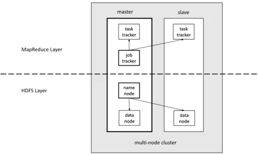
Used by 60% of the Fortune 500 companies, Hadoop has become the industry standard for dealing with big data problems. The Hadoop implementation of MapReduce can be described as a cluster of TaskTracker nodes, dealing with a JobTracker and client node, see Figure 2.6. Once a MapReduce application has been created, the job is committed to Hadoop and then passed to the JobTracker which initialises it on the cluster. During execution, the JobTracker is responsible for managing the TaskTrackers on each node and each TaskTracker spawns Map and Reduce tasks depending on the JobTraker’s requirements [26]. Inputs to the Map tasks are retrieved from the Hadoop distributed file system (HDFS), a shared file system that ships with Hadoop. These inputs are partitioned into multiple splits which are passed to the map tasks. Each split contains a small part of the data that the Map function will operate on. The Map results are sorted and passed to the Reduce tasks. The results of the Reduce tasks are written back to HDFS where they can be retrieved by the user [6].
In a small Hadoop cluster, there is only one single master with multiple slave nodes. As shown in Figure 2.6, the master contains JobTracker, TaskTracker, NameNode and DataNode. But the slave nodes only contains a DataNode and TaskTracker. They are managed and controlled by the NameNode and JobTracker of master node. The small-scale Hadoop cluster is used only in nonstandard applications [29].
task tracker job tracker name node data node master slave task tracker data node MapReduce Layer HDFS Layer multi-node cluster
Figure 2.6: Overview of a multi-node Hadoop cluster.
For a larger size cluster, a dedicated NameNode server is assigned to manage HDFS with file system index. The secondary NameNode duplicates the structure of master NameNode as a snapshot. This structure can prevent the file system corruption and reduce the risk of data loss. Similarly the JobTracker server is responsible for job scheduling.
2.3.2 Hadoop Distribution File System
The Hadoop distributed file system (HDFS) is a shared file system developed for the Hadoop framework. In a Hadoop cluster, the NameNode and DataNodes are formed in the HDFS layer (see Figure2.6). Usually the master has both of nodes and slave node only has DataNode, because of the DataNode is not required to be present in each node. The TCP/IP layer is used by the file system for communication between nodes. The interaction of each DataNode is accomplished by using the protocol specific to HDFS [30].
HDFS is distributed, scalable, and portable. It is usually used to stores big data files over multiple machines, which typically can be in the range of gigabytes to terabytes [31]. HDFS achieves reliability by replicating the data files across different nodes. By default, 3 replications of data files are stored on 3 multiple nodes: two copies are on the same rack, and another one is on a different rack [32]. The data nodes are interactive and can reform the data rebalancing.
Using HDFS provides a significant data awareness in file system. The responsibility of JobTracker is to assign the Map or Reduce jobs to TaskTrackers. The data location is aware of while scheduling the jobs. More specifically, each node of the cluster only schedules the Map or Reduce tasks on its own data. For example, node M contains data (a, b) and then node M would only be scheduled to perform Map or Reduce tasks on (a, b). This advantage prevents the unnecessary traffic transfer over the cluster nodes, and reduces the data traffic time. However, this advantage is now always available when Hadoop is used with other file systems. Moreover, Jiong Xie et al. [33] discovered that it significantly impacts the job completion time, demonstrated by running intensive-scale jobs.
HDFS was initially designed for most files except the systems requiring concurrent write-operations [34]. In addition a Filesystem in Userspace (FUSE) interface is included into HDFS, enabling users to write a normal userland application as a bridge for a traditional filesystem interface [35].
2.3.3 HBase
HDFS file system is also the basis of Apache HBase, a column-oriented distributed database management [36]. HBase has become the standard tool for big data storage and query. It originates from Google’s BigTable and is developed as part of the Apache Hadoop project [6]. The instinctive features of HBase are providing the capabilities of querying and storing big data for Hadoop, such as serving database tables as the input and output for MapReduce jobs and real-time data access. Additionally HBase features file compression, in-memory operation and bloom filters [37].
2.3.4 Rhipe Package
Rhipe is a R package that integrates Hadoop within the R programming environment [38]. In other words, Rhipe is a fusion of R and Hadoop, combining the interactive R environment and the highly scalable parallel Hadoop framework, to facilitate the statistical analysis of complex big data [39]. Rhipe uses Hadoop to parallelise the computationally intensive tasks.
This package was developed by Saptarshi Guha from the Purdue Statistics Department [40]. Currently a core development team is established and a Google discussion group is provided to all the users and researchers.
The impressive contribution of Rhipe is that its functionalities are achievable with small-scale data sets [39]. It was initially inspired by two goals. The first goal is to achieve
deep data analysis in an efficient way. Moreover it is more concerned about avoiding data loss which caused by inappropriate data reductions. In order to achieve the first goal for small or big data, the visualised and statistical methods are required to extract the characteristics of data and detailed statistics. Therefore, the second goal is to integrate with the high-level R language, in order to improve the efficiency and effectiveness by avoiding low level programming.
The Rhipe chooses Hadoop to access scalable I/O and parallel the computing. As described above in section 2.3.1, Hadoop was designed for cluster machines to handle the comprehensive computing in a scalable way. It is practical to deal with very different performance characteristics of different operating platforms. The advantages of using Hadoop is not limited to the parallelism of cluster computing over time, but also the detailed tracking record in its open-source application which supported by Apache. Compared to the existing parallel R packages, Rhipe is more beneficial for users in data analysis [39]. In addition, Rhipe is more computationally effective by applying the high capabilities and support of Hadoop. More details are presented in Chapter 4 section 4.3.1.
2.4
Amazon Web Service
Amazon Web Services (AWS) is a cloud computing platform with a collection of remote computing services, served over the Internet. The most well-known services of AWS are Amazon Elastic Compute Cloud (EC2) and Amazon Simple Storage Service (S3) [41]. The significant advantage of utilising AWS is providing an elastic computing service with high capacity. Using AWS services requires less resources and is cheaper than establishing a cloud server in-house.
2.4.1 Elastic Cloud Computing
Amazon Elastic Compute Cloud (EC2) is a pivotal part of AWS cloud platform [42]. EC2 allows users to rent virtual computer resources for running their own computing applications. It also provides the scalable deployment by using AWS’ Amazon Machine Image (AMI) service, which allows user to create and manage a virtual machine with user desired software. In EC2, each virtual machine created by users is called an “instance”. The “elastic” feature of EC2 can be explained as follows: users can create, launch, and terminate the cloud instances based on their needs and only pay for the cost of active running hours of instances. There are three basic EC2 instance types, namely
On-Demand, Reserved and Spot. All types of the instances provides the same standard computing capacity although they may be from different data centres based on the different geographical locations. The only difference between these three types is the different pricing schemes of the instances [42].
In November 2010, Amazon switched its own retail website to EC2 and AWS.
2.4.2 StarCluster
StarCluster is a cluster computing toolkit, specially designed for Amazon’s Elastic Com-pute Cloud (EC2). It is open-source and released under the LGPL license [43].
Using StarCluster, users are able to build, configure and manage the AWS virtual ma-chine clusters in a simpler and more automatic way. Additionally, StarCluster allows users to create a cloud computing environment for parallel computing quickly and easily. The target users group of the StarCluster is the academic researchers with the needs for cluster computing services.
StarCluster is a command-line tool written in Python with an user-friendly interface to AWS EC2. The most beneficial part of StarCluster is that the strong supports of variants EC2 Linux system images.
There are three reasons to build StarCluster specially for AWS. Firstly cloud computing is the future trend for computing service, allowing all the intensive programming works outsourced. AWS is playing the lead role among the existing popular and standard cloud computing platforms. Secondly, in contrast to the different controlling and configuration manager for different AWS services, there is a need for a simple control method over all different commands through a programmable API [43]. Furthermore, with the helps of StarCluster toolkit, systems administrators and programmers can focus more on the researches with a comfortable cloud user environment, rather than spending time on the complicated procedure of managing a big cluster. All of these logistical complications are removed with the development of this easy-to-use command toolkit with an easier access to AWS cloud computing service.
More practical benefits of StarCluster will be introduced and demonstrated in Section 4.2.4.
2.5
Boosting
Boosting is a general method to improve the accuracy of a given set of learning algorithms [44]. The idea of Boosting is to combine a set of learners to form an ensemble in order to achieve a better performance. Assuming that the learning hypotheses can be presented ash1,h2, . . . , hT , and the ensemble hypothesis is a sum of these hypotheses [45]:
f(x) = T X
t=1
αtht(x). (2.2)
The parameter αt is the coefficient of each combined ensemble member ht. The learner
ht is learned with the boosting procedure through the interoperation of αt. Therefore, the hypothesis boosting problem can be simplified and referred to the process of combing a set of weak hypothesises into a strong hypothesis [46]
Boosting was inspired by a machine learning theory called the “PAC” (Probably Ap-proximately Correct) learning model [47], due to Valiant’s the Learnable Theory [48]. Professor Michael Kearns was the first to pose the question “Can a set of weak learners create a single strong learner?” in his hypothesis [46]. Later boosting theory proved that if each base learner performs slightly better than random guess, it is possible to combine them to form an arbitrarily better performing ensemble.
Schapire was the first to provide a polynomial time boosting algorithm [49]. Later he applied the boosting idea to a real-world problem, using the base learners of neural networks for boosting [50].
After the above works appeared, boosting was defined as a learning algorithm, which can generate high-accuracy predictions or estimates using a set of base learners, which in turn can efficiently generate hypotheses slightly better than random guess. In machine learning, a weak learner is defined as a classifier only slightly correlated with the actual target. In contrast, a strong learner is a classifier that is well-correlated with the actual target.
A boosting algorithm can be applied to model fitting, variable selection, and model choice. Compared to the original outcomes from variant learners, the outcome of boost-ing always leads to a better prediction or estimation. In order to improve the predictive quality, boosting is usually considered as an efficient but time-consuming approach for increasing the accuracy of forecasting. More practical theories are introduced and anal-ysed in Section5.1.
2.6
Related Work
Both the processing of times series data and specific time series prediction techniques have been previously studied by different researchers. Hadoop.TS [51] was proposed in 2013 as a toolbox for time series processing in Hadoop. This toolbox introduced a bucket concept which traces the consistency of a time series for arbitrary applications. Sheng et al. [52] implemented the extended Kalman filter for time series prediction using the MapReduce methodology. The framework calculated the filter’s weights by performing the update step in the Map functions, whilst the Reduce function aggregated the results to find an averaged value.
A Hadoop based ARIMA prediction algorithm was proposed and utilised for weather data mining by Li et al. [53]. The work describes a nine step algorithm that employs the Hadoop libraries, HBase and Hive, to implement efficient data storage, management and query systems. Stokely et al. [54] described a framework for developing and deploying statistical methods across the Google parallel infrastructure. By generating a parallel technique for handing iterative forecasts, the authors achieved a good speed-up.
The work presented in this thesis differs from previous work in three key areas. First, it presents a low-overhead dynamic model for processing irregularly sampled time series data in addition to regularly sampled data. Secondly, the proposed framework allows applying multiple prediction methods concurrently as well as measuring their relative performance. Finally, it offers the flexibility to add additional standard or user-defined prediction methods that automatically utilise all of the functionalities offered by the framework.
In summary, the proposed framework is mainly focused on effectively applying the Hadoop framework for time series rather than the storage of massive data. The main objective of this thesis is to present a fast prototyping architecture to benchmark and backtest rolling time series prediction algorithms. To the best of authors knowledge, this is the first study focusing on a systematic framework for rolling window time series processing using MapReduce methodology.
Rolling window time series
prediction using MapReduce
To achieve the parallelism of rolling processing in time series, this chapter proposes a methodology to facilitate retrieval and rolling window prediction of irregularly sampled large-scale time series data, using MapReduce Framework. Special issues of rolling analysis in time series data are discussed and straightforward implementation issues arising as a result of proposed framework with a significant improvement on efficiency. Although using Hadoop in the traditional way is not suitable for rolling analysis, there are still variant advantages of implementing the rolling time series prediction in Hadoop, which is considered as the best option so far. Time stamps is the unique feature of time series data, which can be used as an indicator/indexer of locating the indices of data. The notion of index pool is designed to locate the overlapping data which across two adjacent windows.
3.1
Issue of Rolling Analysis using Hadoop
As stated in Chapter 2, the rolling time series processing is to fit the target algorithm on the sample data of a fixed window length. The unique feature of time series data leads the analysis depend on the order of timely manner. Specifically, the sample data in each window is partially overlapping with the adjacent windows. This intrinsic feature does not influence much on the predictions of rolling window time series sequentially, due to that the entire sample data is accessible to be partitioned into splits. MapReduce is originally designed to run Map and Reduce functions concurrently and without any dependencies. Therefore, a technique is needed to locate the overlapping data from neighboring data file precisely and assemble them. This is the core difficulty associated
with this research. The time series bucket concept inspired us to solve this issue with the notion of index pool.
3.2
Proposed Methodology
While financial time series are often recorded in irregular ticks, many forecasting algo-rithms expect a periodic time series. In order to make a time series periodic and/or reduce its temporal resolution, an optional normalization of data may be required in preprocessing stage. This is achieved by applying a user supplied algorithm to rolling windows of the aggregated data.
In the proposed framework, it is assumed that the numerical samples and their times-tamps are stored on HDFS before data input invoking. Then with the introduction of an index pool, a table of time series indexing and time-stamp information for the entire file directory in HDFS is stored in it. The major contribution ofindex pool to the entire framework is being used to assign the appropriate index keys to time series entries, to grantee an appropriate and precise distribution while data across multiple splits. As a result, the index pool is considered the core of the architecture.
Data aggregation and pre-processing are handled by themap function. The aggregated data is then indexed using the index pool and is assigned a key, such that window parts spread across multiple splits are assigned the same unique key. If all of data for a window is available in themapfunction, the prediction is performed and its performance (in terms of prediction error) is measured; the prediction result along with its keys is then passed to the reduce. Otherwise, the incomplete window and its key are directly passed to thereduce, where they are combined accordingly with the partial window from other splits into proper rolling windows. Prediction for these windows is performed in thereduce. The final output is created by combining the results of all prediction.
The pseudocode below illustrates the detailed steps of proposed algorithm in both of Map and Reduce stages, which process the rolling window prediction with window length
l.
Map Stage:
fordata file in [f ile1, . . . , f ilem]do
fID = file ID in index pool
fetch the index list corresponding fID
partition the sample data into windows with l length
if W is a complete window then: predict f(W, otherparams)
return < K, P redictions >to Reduce
else
return < K, IncompleteW indows >to Reduce
end if end for end for
Reduce Stage:
for< K, V > in Map Resultsdo
if for the sameK has multiple vales V then:
assemble the incomplete windows together and sort in right order predictf(W, otherparams) with the assembled complete window return< K, P redictions >
else
reorder the results with keyK end if
end for
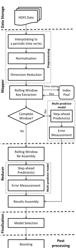
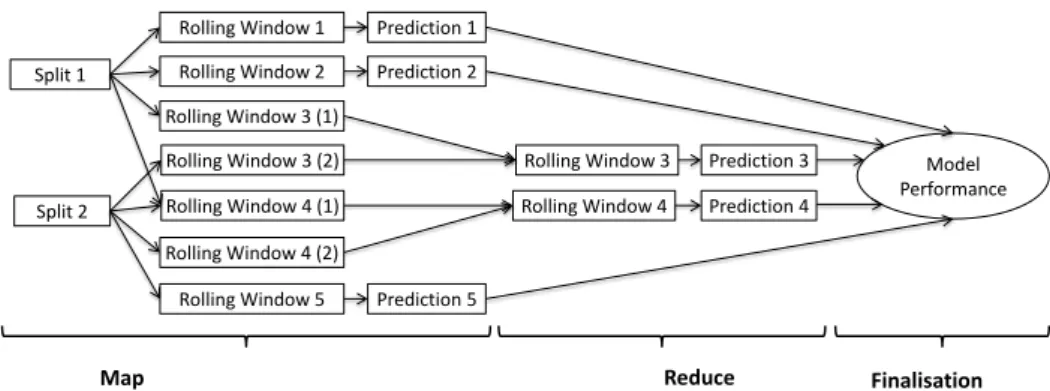
Figure3.1presents the work flow and the architecture of the proposed system. There are five stages in the entire system working flow. The Data storage procedure is processed in HDFS; Mapper and Reducer functions are responsible for the rolling processing of time series prediction; the final outcomes and error measures are taken in Finalisation stage; finally there is a post-processing step to facilitate the boosting of predictions. Figure 3.2shows how the data flows through the blocks. As the logistic design in both Map and Reduce stages, the different procedures of rolling processing facing complete and incomplete windows are clearly illustrated in the diagram. The complete windows are being processed straightforward in Map stage; however, incomplete windows are assembled and process afterwards in Reduce stage. All results are sorted and aggregated in Finalisation session of the working flow.
The rest of this section describes the system components in greater detail, and two different architecture designs are discussed later. The last step of the architecture, boosting, is described separately in Chapter5.
Rolling Window Key Extraction Normalisation Interpolating to a periodic time series
Dimension Reduction Rolling Window Re-Assembly Step-ahead Predictor(s) Error Measurement Model Selection Index Pool HDFS Data Time-stamp Key Mapp er R edu cer Finali sa tio n Da ta St o rag e Step-ahead Predictor(s) Error Measurement Complete Window? Yes No Results Assembly Multi-predictor model M u lti -p re d ict or m od el P re pr oce ssing
Boosting processingPost
Rolling Window 1 Rolling Window 2 Rolling Window 3 (1) Rolling Window 3 (2) Rolling Window 4 (1) Rolling Window 4 (2) Rolling Window 5 Split 1 Split 2 Rolling Window 3 Rolling Window 4 Prediction 1 Prediction 2 Prediction 3 Prediction 4 Prediction 5 Map Reduce Model Performance Finalisation
Figure 3.2: Flow of data in the proposed framework.
3.3
Design
3.3.1 Data Storage and Index Pool
In the proposed system, the assumption that time series are stored sequentially in mul-tiple files is made as a pre-request. Files stored cannot have overlapping time-stamps and are not necessarily separated at regular intervals,and the lengths of the files are not necessarily same as well. Each sample in time series contains the data and its associated time stamp. The name of each file stored in HDFS is the first time-stamp in a ISO 8601 format, which can easily locate the target files and data access.
The major properties of Index pool designed in the proposed system are only File Name, Start Time-stamp, End Time-stamp and Index List (the length of the files). These basic components can be retrieved, and other additional components could be added if required for special needs. It is represented as a global table that can be accessible over the entire processing procedure, as stored in same file directory (HDFS for example). This Index pool significantly improved the traceability of time series sample while rolling analysis is under processing, in order to avoid the loss of overlapping data across multiple files. Table3.1shows an example of an index pool.
Table 3.1: Example of an index pool
File Name Start Time-stamp End Time-stamp Index List 2011-01-01 2011-01-01 00:00 2011-01-01 22:00 1 → 12 2011-01-02 2011-01-02 00:00 2011-01-02 22:00 13 → 24 2011-01-03 2011-01-03 00:00 2011-01-03 22:00 25 → 36 2011-01-04 2011-01-04 00:00 2011-01-04 22:00 37 → 48 2011-01-05 2011-01-05 00:00 2011-01-05 22:00 49 → 60
The index pool enables arbitrary indices to be efficiently located and is used to detect and assemble adjacent windows. Interaction of the index pool with the MapReduce framework is illustrated above in Figure3.1
Index pool creation is performed in a separate maintenance step prior to forecasting. Assuming that data can only be appended to the filesystem (as is the case for HDFS), index pool updates are trivial, as time series data is a continuous signal in real world.
3.3.2 Preprocessing
Work in the map function starts by receiving a split of data. A preprocessing step is performed on the data, with the following goals:
• Creating a periodic time series: In time series prediction, it is usually expected that the sampling is performed periodically, with a constant time-difference of ∆t
between consecutive samples. If the input data is unevenly sampled, it is first interpolated into an evenly sampled time series. Different interpolation techniques are available, each with their own advantage [55]. Linear interpolation is one of the commonly used techniques [56].
• Normalisation: Many algorithms require their inputs to follow a certain distribu-tion for optimal performance. Normalisadistribu-tion preprocessing adjusts statistics of the data (e.g. the mean and variance) by mapping each sample through a normalising function.
• Reducing time-resolution: Many sampled datasets include very high frequency data (e.g. high frequency trading), while the prediction use-case requires a much lower frequency. Alsothe curse of dimensionality prohibits using high dimensional data in many algorithms. As a result, users often aggregate high frequency data to a lower dimension. Different aggregating techniques include averaging and ex-tracting open/high/low/close values as used in financial Technical Analysis from the aggregated time frame.
3.3.3 Rolling Windows
Following preprocessing, the map function tries to create windows of length W from data{yi}, i= 1,· · ·, l, wherelis the length of data split. As explained earlier, the data for a window is spread across 2 or more splits starting from the samplel−W+1 onwards and the data from anothermapper is required to complete the window.
To address this problem, themap function uses the index pool to create window index keys for each window. This key is globally unique for each window range. The map function associates this key with the complete or partial windows as tuple ({yj}, k), where{yj} is the (partial) window data and kis the key.
In the reduce, partial windows are matched through their window keys and combined to form a complete window. The keys for already complete windows are ignored. In Figure 3.2, an example of partial windows being merged is shown.
In some cases, including model selection and cross-validation, there is no need to test prediction algorithms on all available data; Correspondingly themap function allows for arbitrary strides in which every mth window is processed.
3.3.4 Prediction
Prediction is performed within amulti-predictor model, which applies user all of supplied predictors to the rolling window. Each data window {yi}, i = 1,· · · , w is divided into two parts: the training data with {yi}, i= 1,· · ·, w−h, and{yi}, i=w−h,· · · , w as the target. Separation of training and target data at this step removes the possibility of peeking into future from the architecture.
The training data is passed to user supplied algorithms and the prediction results are returned. For each sample, the time-stamp, observed value and prediction results from each algorithm are stored. For each result, user-defined error measures such as an L1 (Manhattan) norm, L2 (Euclidean) norm or relative error are computed.
To reduce software complexity, the initial design is to perform all the predictions in the reduce, regardless of the concerns whether the sample data is from an incomplete window or complete window; however, thisstraightforward method is inefficient due to the MapReduce architecture. In the Result section there is a detailed comparison of these two designs and a demonstration on the advantages of proposed design. Therefore in our proposed framework only partial windows are predicted in thereduce after reassembly. Prediction and performance measurement of complete windows are performed in the map, and the results and their index key are then passed to the reduce.
3.3.5 Finalisation
In the reduce, prediction results are sorted based on their index keys and concatenated to form the final prediction results. The errors of each sample are accumulated and converted to a summary error measures, allowing model comparison and selection.
Commonly used measures are Root Mean Square Error (RMSE), Mean Absolute Pre-diction Error (MAPE) and Symmetric mean absolute percentage error (SMAPE):
RMSE(Y,Yˆ) = v u u t 1 N N X i=1 (yi−yˆi)2 (3.1) MAPE(Y,Yˆ) = 1 N N X i=1 |yi−yˆi yi | (3.2) SMAPE(Y,Yˆ) = 1 N N X i=1 |yˆi−yi| (|yi|+|yˆi|)/2 (3.3)
where Y = [y1,· · · , yN] is the observed time series, ˆY = [ˆy1,· · ·,yˆN] is the prediction result andN is the length of the time series.
The SMAPE measure is not recommended as a measure of forecast accuracy since small values of the denominator lead to division by numbers close to zero [57]. However, since it is in widespread use, it is included in the results.
Akaike Information Criterion (AIC) is another measure, and is widely used for model selection. AIC is defined as:
AIC = 2k−2 ln(L) (3.4) wherek is the number of parameters in the model andL is the likelihood function.
3.4
Forecasting
3.4.1 Multi-Predictor Model
In this section, some of popular time series prediction algorithms are described, which are used as the predictor models of the experimental results in Chapter6. In addition, a multi-predictor model (MPM) scheme is applied to the proposed framework for the automatic selection of an appropriate prediction model. MPM is expected to improve the efficiency of batching predictors. In this scheme, the multi-predictor function is called in the Map or the Reduce, which in turn applies all user supplied predictors to each data window, returning a vector of prediction results (and error measures) for every predictor. Following the MapReduce, MPM selects the most proper predictor for the particular test time series by comparing the error measures (RMSE and MAPE) of each prediction model, which are illustrated in Finalisation section.
3.4.2 Linear Autoregressive Models
Autoregressive (AR) models are a type of statistical process where any new sample in a time series is a linear function of its past values. Because of their simplicity and gener-alisability, AR models have been studied extensively in statistics and signal processing and many of their properties are available as closed form solutions [11].
3.4.2.1 AR model
A simple AR model is defined by:
Xt=c+
p X
i=1
φiXt−i+t (3.5)
where Xt is the time series sample at time t, p is the model order, φ1, . . . , φp are its parameters,c is a constant and t is white noise.
The model can be rewritten using the backshift operatorB, where Bxt=xt−1:
(1−
p X
i=1
φiBi)Xt=c+t (3.6)
Fitting model parameters φi to data is possible using the least-squares method. How-ever, finding the parameters of model for data X1, . . . , XN, requires the model order
p to be known in advance. This is usually selected using AIC. First, models with
p ∈[1, . . . , pmax] are fitted to data and then the the model with the minimum AIC is
selected.
To forecast a time seriesX1, . . . , XN, first a model is fitted to the data. Using the model, predicting the value of the next time-step is possible by using Eq. 3.5.
3.4.2.2 ARIMA models
The autoregressive integrated moving average (ARIMA) model is an extension of AR model with moving average and integration. An ARIMA model of order (p, d, q) is defined by: 1− p X i=1 φiBi ! (1−B)dXt=c+ 1 + q X i=1 θiBi ! t (3.7)
wherepis autoregressive order,dis the integration order,q is the moving average order andθi is theith moving average parameter. Parameter optimisation is performed using Box-Jenkins methods [11], and AIC is used for order selection.
AR(p) models are represented by ARIMA(p,0,0). Random walks, used as Na¨ıve bench-marks in many financial applications are best modelled by ARIMA(0,1,0) [58].
3.4.3 NARX Forecasting
Non-linear auto-regressive models (NARX) extend the AR model by allowing non-linear models and external variables being employed. Support vector machines (SVM) and Artificial neural networks (ANN) are two related class of linear and non-linear models that are widely used in machine learning and time series prediction. More details about the algorithms are going to be elaborated as below:
3.4.3.1 ETS
Exponential smoothing state Space (ETS) is a simple non-linear auto-regressive model. ETS estimates the state of a time series using the following formula:
s0 =X0
st=αXt−1+ (1−α)st−1
(3.8)
wherestis the estimated state of time seriesXtat timetand 0< α <1 is the smoothing factor.
Due to their simplicity, ETS models are studied along with linear AR models and their properties are well-known [11].
3.4.3.2 SVM
SVMs and their extension support vector regression (SVR) use a kernel to map input samples to a high dimensional space, where they are linearly separable. By applying a soft margin, outlier data is handled with a penalty constant C, forming a convex problem which is solved efficiently [59]. As a result, there are several models using SVM that have been successfully studied and used in time series prediction [60].
In this thesis, a Gaussian radial basis kernel function was used:
k(xi, xj) = exp − 1 σ2||xi−xj|| 2 (3.9)
where xi and xj are the ith and jth input vectors to the SVM, and σ is the kernel parameter width.
The time series NARX model using SVM is defined as:
Xt=f(C, σ, Xt−1,· · · , Xt−w) (3.10)
wheref is learnt through the SVM andwis the learning window length.
To successfully use SVM for forecasting, its hyper-parameters including penalty constant
C, kernel parameter σ and learning window length w have to be tuned using cross validation. Ordinary cross validation cannot be used in time series prediction as it reveals the future of the time series to the learner [11]. To avoid peeking, the only choice is to divide the dataset into two past and future sets, then train on past set and validate on future set.
The following algorithm is used to perform cross-validation:
forw in [wmin, . . . , wmax]do prepare X matrix with lag w
training set ← first 80% of X matrix testing set ← last 20% ofX matrix
for C in [Cmin, . . . , Cmax]do
forσ in [σmin, . . . , σmax]do
f ← SVM(C,σ, training set) err ← predict(f, testing set)
if err is best so farthen: best params ← (C, σ, w)
end if end for end for end for
return best params
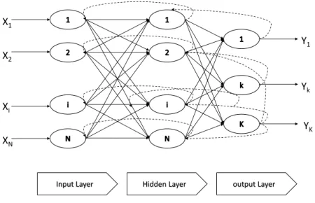
3.4.3.3 Artificial Neural Networks
Artificial neural networks (ANN) are inspired by biological systems. An ANN is formed from input, hidden and output node layers which are interconnected with different weights. Each node is called a neuron.
Similar to SVM, ANNs have been extensively used in time series prediction [61]. In an NN autoregressive (NNAR) model, inputs of the network is a matrix of lagged time series, and the target output is the time series as a vector. Back-propagation neural network
X1 X2 Xi XN Y1 Yk YK
Input Layer Hidden Layer output Layer
Figure 3.3: The back-propagation neural network structure
is a learning algorithm used to minimise error of this network’s output. Basically back-propagation NN weights the connected neural neuron by gradient decent method. The structure of a back-propagation ANN is shown in Figure 3.3. The solid lines are the forward moves and dot lines are the training connection moves. In the output layer, each neuron’ output is aggregated by the previous level’s neurons multiplied by their corresponding weights [62].
Xiao and Chandrasekar successfully applied back-propagation ANNs for e-commerce customers patterning and rainfall estimation from radar data separately [63]. In this thesis, a feed-forward ANNs with a single hidden layer is used for the experiments, the structure is similar as the picture show in Figure3.3.
f(x) =g( N X
i=1
wixi) (3.11)
wherexi is the value of neuron and the weights of each levelwi, andg(y) is the activation function.
3.5
Summary
In this chapter, the proposed methodology was demonstrated in detail after raising the issue of rolling time series analysis using Hadoop. It includes how the new data storage index design,index pool, was formed, and how rolling windows smoothly proceed
using MapReduce model. The rest of this chapter presented the multi-predictor model developed for automatic algorithm selection and the details of each forecasting algorithm used in the proposed framework.
Cloud-based Platform
Another objective of this work is to deploy the the framework on a cloud-based envi-ronment. This chapter provides a comparison of the state-of-art in commercial cloud services, including Amazon Web Service and Microsoft (Windows) Azure, particularly with respect to their ability of supporting the large-scale experiments. Other essen-tial aspects such as price and storage services are also considered. The Rhipe software framework is chosen to provide the development environment for the parallelism of the proposed framework. In this chapter, the practical example of Rhipe and its advantages are demonstrated in detail.
4.1
Cloud Platform
The shift to cloud computing is a major change for businesses and industries. Cloud computing is defined as a system where software applications may be run in an envi-ronment consisting of a logically abstract network of general purpose computers [64]. Following the definition, there are numerous benefits offered by a cloud-based platform, i.e. (1) lets developers create apps which are available to users anytime and anywhere; (2) provides self-service access to a variety of computing resources; (3) enables an elastic control of resources allocation; (4) only charges for the resources users used.
There are two major use-cases of a cloud-based platform: computing and storage (see Table4.2). From the development viewpoint, developers currently categorise the differ-ent levels of cloud computing services to IaaS (Infrastructure as a Service) and PaaS (Platform as a Service).
4.1.1 Comparison of Different Cloud Platform
Generally a cloud-based platform can be easily utilised without physical room space, regular maintenance, front-end investment in machines and other facilities. As a result of market demand and technological innovations, several cloud platform service providers have been established in recent years.
In this chapter, two of the most prevalent cloud services are studied:
• Amazon Web Services
AWS plays a leading role in the constant innovation and enhancements to the service. AWS now has provided 30 services ranging from basic cloud computing to real-time data storage all across the world since 2006. Major services cover the area of compute, networking, storage & content delivery, database, App services, mobile services and applications. There are a variety of computing resources and instance types offered to meet the unique needs of different user groups. AWS has established 8 data centres all over the world in 2014, in order to provide the standard services to the users in different regions [41].
• Microsoft
Microsoft Azure (formerly called Windows Azure) is a cloud computing platform and infrastructure, owned by Microsoft. It provides the cloud resources, applica-tions and services through a global datacentre network. Both PaaS and IaaS ser-vices are supported with many different programming languages, tools and frame-works. Azure was launched in 2010 [65].
Generally these two well-known cloud services provide users with similar and compatible services. They are both of user-friendly interface, allowing users to create and manage the cloud computing environment in a few minutes through simple operations on web browsers. There are minor performance differences between these two providers, but often vary in terms of the machine configuration options and pricing schemes.
Table 4.1and Table 4.2 compare the price and service features between AWS and Mi-crosoft Azure. AWS is slightly cheaper than MiMi-crosoft in tiers with similar configuration. All of the compared prices are studied in the same region (US east) and of the same operating system (Linux). Both options provide similar IaaS and PaaS services, and relational, scale-out and blobs storage. It is found AWS more preferable due to its lower operational cost.
Table 4.1: Price comparison of Amazon and Microsoft
Instance Virtual CPUS RAM Cost per hour
Amazon m3.medium 1 3.75GB 7 cents
Amazon m3.large 2 7.5GB 14 cents
Amazon m3.xlarge 4 15.00GB 28 cents Amazon m3.2xlarge 8 30.00GB 56 cents Microsoft Azure Medium A2 2 3.50GB 15.4 cents
Microsoft Azure Large A3 4 7.00GB 30.8 cents Microsoft Azure Extra Large A4 8 14.00GB 61.6 cents
Table 4.2: Service comparison of Amazon and Microsoft
Name Computing Storage
Iaas Paas Relational Scale-out Blobs Microsoft Hyper-V
Cloud
Windows Azure
SQL Azure Azure Tables Azure Blobs Amazon EC2 Elastic
Beanstalk
RDS SimpleDB S3
4.2
AWS
4.2.1 Elastic Compute Cloud
Amazon Elastic Compute Cloud (Amazon EC2) is briefly introduced in Chapter2which is the central service of AWS, providing resizable computational cloud resources. AWS EC2 has a simple web service interface for users to manage and control the com-puting properties easily and quickly. It provides complete controls of the comcom-puting resources and lets users run on Amazon’s proven computing environment. The time of creating and booting new cloud computing resources is significantly reduced by using AWS EC2. AWS EC2 enables the quick scaling on computing capacity as the user re-quirements change, hence it is “elastic�