The Application of Divergences in Prototype Based Vector Quantization
Haase, Sven
IMPORTANT NOTE: You are advised to consult the publisher's version (publisher's PDF) if you wish to cite from it. Please check the document version below.
Document Version
Publisher's PDF, also known as Version of record
Publication date: 2014
Link to publication in University of Groningen/UMCG research database
Citation for published version (APA):
Haase, S. (2014). The Application of Divergences in Prototype Based Vector Quantization [S.l.]: [S.n.]
Copyright
Other than for strictly personal use, it is not permitted to download or to forward/distribute the text or part of it without the consent of the author(s) and/or copyright holder(s), unless the work is under an open content license (like Creative Commons).
Take-down policy
If you believe that this document breaches copyright please contact us providing details, and we will remove access to the work immediately and investigate your claim.
Downloaded from the University of Groningen/UMCG research database (Pure): http://www.rug.nl/research/portal. For technical reasons the number of authors shown on this cover page is limited to 10 maximum.
Prototype Based Vector Quantization
Prototype Based Vector Quantization
PhD thesis
to obtain the degree of PhD at the
University of Groningen
on the authority of the
Rector Magnificus Prof. E. Sterken
and in accordance with the decision by the College of Deans.
This thesis will be defended in public on
Friday 28 March 2014 at 12.45 hours
by
Sven Haase
born on 16 May 1983
in Zschopau, Germany
Prof. M. Biehl Prof. T. Villmann Assessment committee Prof. W. H. Hesselink Prof. J. C. Principe Prof. F. Rossi ISBN: 978-90-367-6864-1
Acknowledgements ix
1 Introduction 1
1.1 Scope . . . 3
1.2 Outline . . . 4
2 Introductory Remarks on Entropies 7 2.1 Definition and Interpretation of Shannon Entropy . . . 7
2.1.1 Shannon Entropy . . . 7
2.1.2 Shannon Differential Entropy . . . 10
2.1.3 Relative Entropy and Mutual Information . . . 11
2.1.4 Interpretations of the Shannon Entropy . . . 13
2.2 Definition and Interpretation of R´enyi Entropy . . . 14
2.2.1 R´enyi Entropy . . . 14
2.2.2 Geometric Interpretation of R´enyi Entropy . . . 15
2.3 Other Measures of Entropy . . . 16
3 A Systematic Characterization of Divergence Measures 19 3.1 General Remarks on Divergences . . . 20
3.2 Bregman Divergences . . . 21
3.2.1 General Definition and Fundamental Properties . . . 21
3.2.2 Bregman Geometry . . . 23
3.2.3 Important Representatives of Bregman Divergence . . . 25
3.3 Csisz´ar’sf-Divergences . . . 27
3.3.1 General Definition and Fundamental Properties . . . 27
3.3.2 Important Representatives off-Divergence . . . 31 v
3.4 γ-Divergences . . . 34
3.5 Metric Divergences . . . 36
3.6 A General Relation Between Entropies and Divergences . . . 38
3.7 Discussion of Divergences . . . 38
3.7.1 Linear Monotonically Increasing Noise . . . 40
3.7.2 Additive Uniform Noise . . . 41
4 Derivatives of Divergences - a Functional Analytic Approach 45 4.1 Functional Derivatives - Fr´echet-Derivatives . . . 45
4.2 Fr´echet-Derivatives for the Different Divergence Classes . . . 47
4.2.1 Bregman-Divergences . . . 47
4.2.2 f-Divergences . . . 48
4.2.3 γ-Divergences . . . 49
4.3 Derivatives for Hyperparameter Learning . . . 50
4.4 Fr´echet-Derivatives for Relevance Learning . . . 51
5 Notes on Vector Quantization and the Use of Divergences 53 5.1 Unsupervised Vector Quantization . . . 54
5.1.1 Basic Methods . . . 54
5.1.2 Self-Organizing Maps . . . 55
5.1.3 Neural Gas . . . 56
5.1.4 Exploration Machine and Further Vector Quantization Ap-proaches . . . 57
5.2 Simulations for Unsupervised Vector Quantization . . . 58
5.3 Magnification . . . 64
5.3.1 Magnification Control . . . 65
5.3.2 Simulations . . . 66
5.4 Supervised Vector Quantization . . . 68
5.4.1 Basic LVQ algorithms . . . 68
5.4.2 Advanced Learning Vector Quantization . . . 71
5.5 Simulations for Learning Vector Quantization . . . 71
5.6 Extensions for the Basic Adaptation Scheme . . . 76
5.6.1 Hyperparameter Learning . . . 76
5.6.2 Relevance Learning . . . 77
6 Kernelized Vector Quantization in Online-Learning 81 6.1 Kernel, Kernel Distances and Kernel Mapping for Gradient Based VQ 82 6.2 Universal Kernels Based on Divergences . . . 86
6.3 Exemplary Applications . . . 87
6.3.1 The Artificial Dataset - Palau Flag Dataset (PFD) . . . 87 vi
6.3.2 Human-Avatar Dataset (HAD) . . . 88
7 SNE for Dimension Reduction and Visualization Using Arbitrary Diver-gences 91 7.1 Review of SNE and t-SNE . . . 92
7.2 Derivation of the General Cost Function Gradient for t-SNE and SNE 94 7.2.1 The Generalized t-SNE Gradient . . . 94
7.2.2 The Generalized SNE Gradient . . . 96
7.3 t-SNE Gradients for Several Divergences . . . 98
7.3.1 Bregman Divergences . . . 98
7.3.2 Csisz´ar’sf-Divergences . . . 99
7.3.3 γ-Divergences . . . 101
7.3.4 Exemplary Simulations . . . 102
8 Summary and concluding remarks 107
Publications 113
Appendix A Boundedness forf-Divergences 119
Appendix B Calculation of the Derivatives of Divergences with Respect to
the Hyperparameters 121
Appendix C Tables 127
Nederlandse samenvatting 133
Bibliography 137
At the end of the journey it is time to thank all the amazing people who made this thesis possible in the first place. Since this work arose foremost in free time beside my regular job, this never would have been possible without the tremendous help and support from those people.
First and foremost I express my sincerest gratitude to my supervisor, Prof. Thomas Villmann, who always supported me and pushed me to go ahead. He is not only a highly committed supervisor but also a true friend.
My deep appreciation goes to Prof. Michael Biehl for his guidance and his assis-tance fighting the Dutch bureaucracy. His ability to find the right words at the right time did me a lot of good in the final phase of this thesis.
In addition, I would like to thank all my co-authors for their valuable support and important contributions to our joint publications. I am especially grateful for the fruitful collaboration and the stimulating discussions with Dr. Kerstin Bunte and Ernest Mwebaze. Furthermore my special thanks goes to all members of the Com-putational Intelligence Group Mittweida for many lively discussions and a great time along the way. I am thankful to the members of the assessment committee for the attentive remarks that helped to further improve the manuscript. In addition, I deeply acknowledge Harm de Vries for translating the summary to Dutch.
Furthermore I would like to thank my employers Prof. Sven Rzepka, Dr. Norbert R ¨ummler, and Bettina Seiler for providing me sufficient flexibility during finaliza-tion of this thesis.
Even though they are hardly aware of their helpful and stimulating role I am thankful to my parents, my parents-in-law, and my friends for being available for me whenever needed. Finally, without the support of my beloved wife Isabell and my wonderful children Melia and Talina I would never have succeeded. Although they often had to endure my absence they were completely understanding and en-couraged me with their patience and unconditional love.
Sven Haase ix
Introduction
N
owadays we are faced with a huge amount of data in our daily lives and in ourprofessions at any time. Even for us humans, it is not always easy to extract the essential information from these data. This raises the question: ’How can we program a machine to learn automatically from data and to improve with experi-ence?’ Learning in this context is extracting information directly from data,mean-inglearning-from-examples. That implies the recognition of complex patterns and the
deduction of intelligent decisions based on data.
The key objective ofmachine learningis to answer the aforementioned question. Therefore, the broad field of machine learning develops algorithms that identify the key information from data samples and experience. This learning from examples scenario starts with a data set which globally conveys information about a real-world event, and the goal is to capture the information in the parameters of a learn-ing machine (Principe et al. 2000). This machine learnlearn-ing problem often involves an adaptation process, where the parameters of the learning system are adjustable in such a way that performance improves through repeated presentation of exemplars to the system (Jenssen 2005). These adaptive systems require some criterion to com-pare how similar two samples are. The Euclidean metric is the most common choice as a measure of dissimilarity.
Recently, however, information-theoretic criteria have been developed for many machine learning approaches to judge their performance. The concept of
informa-tion theoretic learning(ITL) as a general framework for machine learning and the
training of adaptive systems using information theoretic criteria was introduced by Principe et al. (2000). They proposed the utilization of information theory, because it is the best possible approach to deal with manipulation of information (Shannon and Weaver 1949).
Machine learning in general covers a broad range of data processing methods, e. g. for blind source separation, feature extraction, dimensionality reduction, clus-tering and classification. In a general sense one can distinguish three different learning paradigms: unsupervised learning, supervised learning and reinforcement learning.
The objective ofunsupervised learningwithin the meaning of clustering is to group unlabeled data into groups of similar objects, so-called clusters. On the other hand, prominent supervised learning algorithms utilize labeled data during the training process to get a so called classifier which enables a subsequent classification of un-known data samples. Reinforcement learning is characterized by a clever trade-off between exploration and exploitation to discover actions that maximize a delayed reward (Sutton and Barto 1998).
This thesis focuses on supervised learning and unsupervised learning and in particular on vector quantization. Many approaches to both learning paradigms have the common idea to quantize the data by a set of prototypes. Popular unsu-pervised prototype-based methods are, for example c-Means (Ball and Hall 1967), the Self Organizing Maps (SOM) (Kohonen 1990b) and Neural Gas (NG) (Martinetz et al. 1993). Well known prototype-based classification methods are Support Vec-tor Machines (Steinwart and Christmann 2008) and Learning VecVec-tor Quantization (LVQ) (Kohonen 1986).
Independent from the learning paradigm, classification and clustering is always strongly associated with the concept of dissimilarity. However, the traditionally used Mean Squared Error (MSE) sometimes seems to be insufficient to extract the structure of the data. To tackle these limitations, information theoretic concepts for machine learning have been proposed in recent years. One important information theoretic property of vector quantizers which describes the relation between data probability density and prototype vector density is the so-called magnification. Us-ing this property, we can state whether a vector quantizer works optimally in infor-mation theoretic sense (Zador 1982). If so, the mapping is able to transfer optimal information from the input data to the prototypes (which is equivalent to an optimal coding and almost lossless data compression). However, vector quantizers like SOM or NG are not optimal in that sense. Thus, the knowledge of magnification of a map is essential for correct interpretation of its output (Hammer and Villmann 2003). Additionally, explicit magnification control is desirable for the learning algorithm if (depending on the respective application) only sparsely covered regions of the data space have to be emphasized or, conversely, suppressed (Villmann 2005, Villmann and Claussen 2006).
However, controlling the magnification factor is only an implicit way in improv-ing information optimality of the mappimprov-ing of the vector quantizer. Moreover, the reason for a sub-optimal mapping of traditional vector quantizers may be attributed to the use of the Euclidean distance as the similarity measure. Due to the global nature of the mean squared error cost function, the prototype update is greatly in-fluenced by outliers, which are the data in the low probability regions. This leads to
oversampling the low probability regions and undersampling the high probability regions by the prototypes (Chalasani 2010). Using information-theoretic descriptors of entropy and dissimilarity (divergence and mutual information) in the learning scheme leads to robustness and generality of the cost function, and improves the performance for many realistic scenarios (fat-tail distributions and severe outlier noise) (Principe 2010). Thus, this gives us an explicit approach to improve the learn-ing machine in an information theoretic sense.
The task of dimension reduction, e. g. compression or embedding of high-dimensional data, is another important problem in machine learning. The objects to be embedded may be either given by high-dimensional vectors or described solely by pairwise dissimilarities. Then the goal of the embedding is to approxi-mate the data distribution, defined by potential neighbors of an object in the high-dimensional input space, as well as possible in a lower-high-dimensional embedding space so as to optimally preserve neighborhood identity for the “images”of the ob-jects (Hinton and Roweis 2002).
As a last point we should mention, that it is not trivial to choose the information optimal dissimilarity measure, even if we have apriori knowledge of the properties of the data. In recent years a huge number of information theoretic dissimilarity measures based on entropy, so-called divergences, have been proposed. These in-formation theoretic criteria capture all the data statistics, since they are functions of probability densities (Jenssen 2005). However, a systematic analysis of machine learning relying on divergences is not given so far.
1.1
Scope
The objective of this thesis is to examine several information theoretic aspects of vec-tor quantization and dimensionality reduction like information-theoretic descrip-tors of entropy and dissimilarity or magnification. Therefore we give a systematic analysis of prototype based online learning schemes rested upon divergence mea-sures. Three main classes of divergences are in the scope of this thesis: Bregman -divergences, Csisz´ar’sf-divergences and γ-divergences. The basic properties for these classes are collected and interconnections between them are pointed out. Fur-thermore, various divergence measures are not only described, it is also shown, how they behave.
Divergences quantify the dissimilarity of probability densities or positive mea-sures. Yet, divergences are neither necessarily symmetric nor have to fulfil the trian-gle inequality as it is supposed for metrics. Nevertheless, some divergences can be
metric under certain conditions. Those distances will be identified, since for some applications it is crucial to have metric dissimilarity measures.
Further, the existing approaches of prototype based information theoretic vector quantizers usually are carried out in the so-called batch mode for optimization but are not available for online learning. A main focus of this thesis is to deduce the mathematical framework for the utilization of divergences in gradient based learn-ing schemes.
Another scope of this work is the application of the proposed methodology for a wide range of algorithms. We demonstrate the utilization of divergences for supervised and unsupervised online vector quantization (considering magni-fication control as well) including SOM, NG, LVQ, stochastic neighbor embedding (SNE) (Hinton and Roweis 2002) and kernel methods using differentiable kernels for Hilbert and Banach spaces.
We remark already at this point, that in vector quantization as well as in learning vector quantization the divergences are used to measure the dissimilarity between specific data points (or data points and prototypes), which are positive measures themselves. In contrast to that, in most applications (as with SNE) divergences are employed to compare the data distribution, i. e. the distribution of several data points.
1.2
Outline
The following chapter 2 starts with a brief discussion of entropy measures, since they occupy a central role in information-theoretic studies. Moreover, the knowl-edge of their properties is essential for the understanding of the behaviour of di-vergence measures, since didi-vergences are based on entropies. Thereby we will es-pecially focus on the well known entropy measures of Shannon and R´enyi. We summarize their essential properties and collate several possible interpretations. A short overview of further measures of entropy will be given as well.
Chapter 3 gives a systematic characterization of divergence measures. For this purpose, three main classes of divergences, theBregman-divergences, theCsisz´ar’s
f-divergences and theγ-divergences, are identified. We review some important representatives of the different divergence-classes and describe their characteristics. An image processing example is discussed for an illustrative demonstration, em-phasizing different properties of the different divergence classes. Thereby, chapter 3 is the first step for a systematic analysis of prototype based clustering and classifi-cation relying on divergences, which is not given yet and is a main objective of this thesis.
The framework of Fr´echet-derivatives will be applied to the several divergences in chapter 4, obtaining generalized derivatives for online learning. Furthermore, the derivatives of several parametrized divergences with respect to the divergence parameter and the derivatives with respect to a weighting function will be given for hyperparameter and relevance learning, respectively. Thus, chapters 2−4 provide all the required foundations for the utilization of divergences in vector quantization. On this basis, in chapter 5 prototype based unsupervised and supervised ap-proaches of vector quantization will be reviewed. Thereby we will focus on the application of divergences as the dissimilarity measure between data points and data points and prototypes, respectively. Here, the data points as well as the pro-totypes are assumed to be positive measures. Simulations using artificial as well as real-world data will be used to demonstrate the potential of divergence based online learning in vector quantization.
A challenging idea in classification learning is the kernel trick. In this approach, the data as well as the prototypes are implicitly mapped into a high-dimensional (may be infinite) feature space which frequently offers a good separation possibility. However, these models are difficult to interpret since the prototypes are living in the may be infinite-dimensional mapping space. If an approximation technique is applied to obtain a finite representation, this leads to an information loss for these models in general. We offer an new approach for the integration of kernels in pro-totype based vector quantization in chapter 6, which provides a new differentiable metric in the data space and thus allows a gradient based learning. Moreover, we re-late information theoretic kernels based on divergences to this concept and demon-strate the abilities and the usefulness of this approach for illustrative examples.
In chapter 7 we propose a framework to apply arbitrary divergences to dimen-sion reduction as used in visualization as well as data compresdimen-sion and fudimen-sion. More precisely, we focus on SNE and t-SNE, which is a variant of the former. SNE ap-proximates the probability distribution in a high-dimensional space (defined by sev-eral neighboring points) with their probability distribution in a lower-dimensional space. Due to the proposed concept, the similarity of the distributions can be quan-tified in terms of arbitrary divergences and hence adapted to user specific require-ments.
Finally, chapter 8 gives a brief summary of the thesis as well as a short discussion of open problems for future investigations.
The major part of this thesis is based on the journal papers (Villmann and Haase 2011, Mwebaze et al. 2011, Bunte et al. 2012, Villmann et al. 2013) and the conference contributions (Villmann, Haase, Schleif and Hammer 2010, Vill-mann, Haase, Schleif, Hammer and Biehl 2010, Mwebaze et al. 2010, K¨astner,
Back-haus, Geweniger, Haase, Seiffert and Villmann 2011, Bunte et al. 2011, Villmann et al. 2011). These articles have been published jointly with several colleagues, as detailed in the list of publications as well as in the bibliography.
Introductory Remarks on Entropies
E
ntropies and divergences are closely related. Since divergences take up a centralposition in this thesis we need a basic understanding of entropy measures as well. In this chapter we give some general remarks and a brief review of entropies. Here we restrict ourselves to entropies which form the basis for the later considered divergences.Entropy measures play an important role in information-theory. The knowledge of their properties is essential for the understanding of the behaviour of divergence measures. For an intuitive introduction we start with the discrete case and discuss the basic properties of the Shannon entropy (Shannon 1948). Thereafter we intro-duce the Shannon differential entropy as well as the relative entropy, the mutual information, and the relationship among these. There are several interpretations of Shannon entropy. We will discuss quite a few of them in section 2.1.4.
In section 2.2 we consider the parametric family of entropies introduced by R´enyi. This flexible measure of uncertainty plays a central role in information the-oretic learning. We will give a statistical as well as a geometrical interpretation of R´enyi entropy.
At the end of this chapter we designate the remaining entropies needed for later definition of divergences, which are Tsallis family of entropies, Burg entropy, Ari-moto’s entropy functions, and the universal class off-entropies.
We remark at this point, that we define the entropy measure for probability den-sity functionspandρ, i. e.R
p(x)dx= 1andR
ρ(x)dx= 1without loss of generality.
2.1
Definition and Interpretation of Shannon Entropy
2.1.1
Shannon Entropy
In the mathematical theory of information one considers an experiment (or a game) with uncertainty in the outcome of the experiment, i. e. it involves the observation of a random variableX. Assume that the possible outcomesx1, x2, . . . , xn of the
P
ipi= 1.
Shannon (1948) defined a quantitative measure,H=H(p1, . . . , pn), of the
uncer-tainty associated with an experiment. Shannon assumed, that such a measure needs to satisfy the following requirements:
1. H is a continuous function of thepi.
2. H(n1, . . . ,1n)attains the maximum value andHis a monotonic increasing func-tion ofn.
3. If a choice is broken down into successive choices, the original quantityH is the weighted sum of the individual values ofH.
The first requirement is obvious since one expects a small change in the uncertainty if a small change in the probabilities occurs. The second assumption is also plau-sible, because for a uniform distribution one has the least information (and hence the maximum uncertainty) on the outcome of the experiment. Clearly, the larger the numbernis, the larger the uncertainty. The third requirement states, that the missing information only depends on the distributionp1, . . . , pnand is independent
of the specific way this information is acquired (independence on the grouping of the events).
Shannon showed that the onlyH satisfying the above requirements is (Shannon 1948, Shannon and Weaver 1949)
H(X) =H(p1, . . . , pn) =−K n
X
i=1
pilogpi, (2.1)
where K is some positive constant. For the sake of simplicity let K = 1in the sequel. We use the convention0 log 0 = 0. H was denotedentropy, since it is the same expression as used to define entropy in statistical mechanics. However, H
is the average uncertainty associated with the possible outcomes of an experiment (Ash 1990) and henceHcan also be interpreted as a measure ofmissing information
(Ben-Naim 2008).
The most important property ofH is that it has it’s maximum if all thepi are
equal. Several other properties of the Shannon entropy can be derived from the three above-mentioned basic properties (Ben-Naim 2008, Cover and Thomas 2006, Jenssen 2005, Principe 2010, Shannon 1948):
• H is a symmetric function of its variables.
• H is a concave1function of its arguments.
1A real-valued functionf :X 7→
Rdefined on a convex setX ⊆ V in a vector spaceV is called
concave, if for allx1, x2 ∈Xand for allλ∈[0,1]the inequalityf(λx1+ (1−λx2))≥λf(x1) + (1−
• His zero iff one event is certain, so that if sayp1= 1andpi= 0, i= 2, . . . nwe
get
H(p1, . . . , pn) = 0. (2.2)
This corresponds to our intuition that the amount of missing information is zero if it is known that one specific event is the only possible outcome of an experiment.
• For two independent random variables,XandY theadditivityproperty holds:
H(X, Y) =H(X) +H(Y), (2.3) whereH(X, Y)is thejoint entropyof a pair of discrete random variables(X, Y)
with a joint distribution.
• Recursivity:
H(p1, p2, . . . , pn) =H(p1+p2, p3, . . . , pn)+(p1+p2)H(p1/(p1+p2), p2/(p1+p2)) (2.4) This recursivity singles out Shannon’s entropy from all the other definitions of en-tropy. More generally,Hsatisfies the composition law, which states that if the sam-ple space is divided into two subsets, the amount of uncertainty with the informa-tion split is the same as it was originally (Majda and Wang 2006).
Figure 2.1 illustrates the Shannon entropy for the simple case of two outcomes
p1=pandp2= 1−p. (HenceH is a function of only on variablep.) The function is concave, it has a maximum atp=12, and it is zero at bothp= 0andp= 1.
Figure 2.1:Shannon entropyH(p)for two outcomes. Here thelogis to the base2and hence
2.1.2
Shannon Differential Entropy
We now extend the concept of entropy to measurable continuous event spaces. For a continuous stochastic variableXwith the corresponding probability density func-tionp(x), the counterpart of equation (2.1) is called the differential entropy, and is given by (Shannon and Weaver 1949)
h(X) =− Z
p(x) log (p(x))dx (2.5)
As in the discrete case, the differential entropy depends only on the probability den-sity of the random variable. Moreover, as we will motivate below, we prefer the continuous approach in this thesis. Hence we meet the following conventions: Remark. For a continuous stochastic variableX with the corresponding probability
den-sity functionp(x)we use the notationH(p)synonymous toH(X). Moreover we use the
notationH(p)for the differential entropy (2.5) and also refer to it simply as entropy in the
following chapters. It should be clear from the context, whether the discrete or the continuous
variant is meant. If confusion can be excluded we use the abbreviationpforp(x).
Consequently, we write the Shannon entropy (2.5) as
H(p) =− Z
plog (p)dx .
Differential entropy can also be interpreted as a measure of uncertainty, and it pos-sesses almost the same properties as the Shannon entropy for discrete variables. But there are two important things to remember. Firstly, for the continuous vari-able case entropy is not bounded from below: Consider a random varivari-ableXwhich is limited to a certain volume v in its space and has a uniform density function
p(x) = 1v = const. Then for v < 1, logv < 0, the differential entropy is neg-ative. If p(x) is the delta function distribution (or a sum of delta functions) the entropy is minus infinity. Secondly, Shannon entropy is not invariant under a vari-able transformation: Assume a smooth invertible transformation fromxtox0. Then
p(x0) =p(x)|dx/dx0|implies thatp(x)dxis invariant butlogp(x)in (2.5) is not. As we adumbrated above, we prefer the functional approach in this thesis due to clarity reasons, a clearer notation and greater flexibility in specific variants of func-tional data processing (Villmann, Haase, Simmuteit, K¨astner and Schleif 2010). We have introduced both, the discrete and the differential entropy because we wanted to sensitize the reader that there is need for some care in extending discrete concepts to continuous variables
2.1.3
Relative Entropy and Mutual Information
Up to now we dealt with the characterization of a single source of information. But the more interesting problem is to compare two sources of information, i. e. to qutify the information content of one probability density function with respect to an-other. One straightforward possibility to measure this information content for two probability densitiesp(x)andρ(x)is the Shannon entropy differenceH(p)−H(ρ). This entropy difference is invariant with respect to a linear transformation but not to a non-linear transformation (Xu 2006) and thus it does not provide a consistent measure of the information content.
Relative Entropy
A measure of the difference between two probability distributions proposed by Kullback and Leibler (1951) is the relative entropy (also called Kullback-Leibler di-vergence)
DKL(p, ρ) =
Z
p(x) logp(x)
ρ(x)dx. (2.6)
It is implicitly based on Shannon’s entropy, since
DKL(p, ρ) =−
Z
p(x) logρ(x)dx−H(p), (2.7) where the quantity
− Z
p(x) logρ(x)dx (2.8)
is commonly denoted as cross entropy betweenpandρ. The relative entropy (2.6) provides a natural and consistent measure of the information content ofpwith re-spect toρsince it is invariant under any smooth invertible variable transformation2.
Herebyρcan be considered as a approximation ofp. We will discuss the Kullback-Leibler divergence and its properties more detailed in chapter 3.
Mutual Information
The relative entropy can be employed as measure of independence between ran-dom variables (Jenssen 2005). LetX, Y be random variables with a joint proba-bility distribution p(x, y) = p(y|x)p(x). It holds, p(x) = R
p(x, y)dy. Moreover,
p(x, y) = p(x)p(y), ifX andY are stochastically independent. The relative entropy
2Note that bothp(x)dxandlogp(x)
ρ(x)in (2.6) are invariant with respect to a smooth invertible
betweenp(x, y)andp(x)p(y)is called the mutual information betweenXandY and is defined as M I(X, Y) = Z p(x, y) log p(x, y) p(x)p(y)dxdy. (2.9)
It quantifies the mutual dependence of the two random variables. The mutual in-formation can be expressed in terms of Shannon entropies using thejoint entropy
H(X, Y) =− Z
p(x, y) logp(x, y)dxdy
and theconditional entropy
H(Y|X) =− Z
p(x, y) logp(y|x)dxdy
as follows (Cover and Thomas 2006):
M I(X, Y) = H(X) +H(Y)−H(X, Y), (2.10)
M I(X, Y) = H(X)−H(X|Y) =H(Y)−H(Y|X). (2.11) From (2.11) one can clearly recognize that the mutual information is the total de-crease in uncertainty inXobservingY (and vice versa). The mutual information is always non-negative, it is zero iff the variables are independent, and it is symmet-ric. The mutual information of a random variable with itself is the entropy of the random variable:
M I(X, X) =H(X)−H(X|X) =H(X).
Figure 2.2 illustrates the relationship among entropy and mutual information.
H(X, Y)
H(X)
H(X|Y) M I(X, Y) H(Y|X)
H(Y)
Figure 2.2:Illustrative representation of the relationship between joint information, entropy,
2.1.4
Interpretations of the Shannon Entropy
There are several possible interpretations of the quantityHand we will only discuss a few of them.
The interpretation as missing informationis very intuitive. Assume one coin is hidden randomly in one ofnboxes. If we are asked to find out in which box the coin is, it is obvious that we lack information on where the coin is hidden. It is also clear that ifn = 1, we do not need any information. Asn increases, so does the amount of information we lack. This interpretation is also reasonable in the case of unequal probabilities. Clearly, any non-uniformity in the distribution increases ones information, and so decreases the missing information.
Another interpretation ofH is closely related to this. Suppose one wants to find the hidden coin using a sequence of “yes or no”questions. Then, the average num-ber of such binary questions needed to find the coin (or generally spoken: to decide on the outcome of an experiment described by a random variableX) can never be less thanH(X).
As curtly mentioned above,H can also be interpreted as the amount of
uncer-tainty(in a probabilistic meaning). Letpi = 1and all otherpj = 0 (j 6=i). Then it
is certain, that the eventioccurred. If the probability ofpidecreases (and thus the
probability of at least onepj increases) one has more uncertainty of the outcome.
The more uniform the distribution is, the more uncertainty one has about the out-come. One can also say thatH measures the average uncertainty that is removed once we know the outcome of a random variable (Ben-Naim 2008). In other words we can say thatH quantifies the expected value of the information contained in a specific realization.
In a more information theoretical context we can give another interpretation for the Shannon entropy, concerning the efficient coding of messages. Assume that a message is generated by a random variableX. Data compression can be achieved by assigning short descriptions to the most frequent outcomes ofX, and necessar-ily longer descriptions to the less frequent outcomes. The Shannon entropyH(X)
gives the shortest average description length of the random variableX. Thus,H
establishes a lower bound on compression rate.
Following Ben-Naim (2008) we recommend to avoid the interpretation ofHas a measure of disorder. First, disorder (or order) is a fuzzy concept and a very subjec-tive term. Second, it does not share the crucial properties ofH. For instance, it is not plausible why the “disorder”of two systems should be the sum of the “disorder”of each system (additivity ofH).
interpretations refer to the whole set of outcomes, not to a single outcome. Shannon entropy is a objective quantity associated with the entire distribution and does not depend on the values of the events. For a more detailed discussion of the several interpretations ofHwe refer to the literature (Ash 1990, Ben-Naim 2008, Cover and Thomas 2006, Shannon 1948).
2.2
Definition and Interpretation of R´enyi Entropy
2.2.1
R´enyi Entropy
A more general class of information measures (compared to Shannon entropy) is the parametric family of entropies introduced by Alfred R´enyi (1961):
HαR(p) =− 1 α−1log Z pαdx =−log Z pαdx α−11 . (2.12) The main structural difference to Shannon entropy is that the R´enyi entropy de-couples the logarithm from its arguments. R´enyi entropy is a very flexible measure of uncertainty (or dissimilarity) due to the parameterα. Figure 2.3 shows the graph of the R´enyi entropyHR
α(p)for the discrete case of two outcomes and differentα
-values. We note that the graph has (for fixedα-value) a quite similar shape as the Shannon entropy had for this example (see figure 2.1). Actually, Shannon entropy
H(p)appears as a special case of the R´enyi entropy:
lim
α→1H
R
α(p) =H(p). (2.13)
Notice that the R´enyi entropy does not satisfy the recursivity property (2.4). All the other fundamental properties of an information measure as postulated for the Shannon entropy (Sec. 2.1.1) are satisfied, including the additivity property for in-dependent probabilities:
HαR(p, q) =HαR(p) +HαR(q) .
Furthermore, R´enyi entropy is invariant with respect to rotations and translations and is maximum for a uniform distribution of random variables having a finite sup-port (Hild 2003).
An important special case is R´enyi’s quadratic entropy, which is
H2R(p) =−log Z
p2dx
=−logE[p(x)]. (2.14) We remark that the argument of the logarithm is theinformation potential
V2(p) = Z
p2dx=E[p(x)],
which is the expectation value of the probability density function (Principe 2010). Generally, one can defineVα(p) =
R
pαdxas theα-moment of the probability func-tionp(x), hence R´enyi entropy is the logarithm of the moment ofp(x).
2.2.2
Geometric Interpretation of R´enyi Entropy
Besides the aforementioned statistical interpretation we will provide a geometric view of R´enyi entropy, which is very useful for the characterization of this family of entropies. Geometrically, probability density functions are points in a function space (referred to as simplex) with the axis given by the random variables. The simplex is the set of all possible probability distributions for a random variable. Figure 2.4 illustrates the simplex for the three-dimensional discrete case. Any point in the simplex is a discrete probability density and has a certain distance to the origin. Let this distance be induced by theα-norm
kp(x)kα= α
s Z
pαdx= pα
Vα(p). (2.15)
Thus, the information potentialVα(p)can be interpreted as theα-norm to the power
ofα. Specifically, R´enyi entropy is theα−1root ofVα(p), rescaled by the negative
of the logarithm as depicted in equation (2.12). Hence,αspecifies the norm in the simplex to measure the distance of p(x)to the origin (Principe 2010) and, conse-quently, changes the importance of small values versus large values in the simplex (as illustrated by figure 2.3).
p1 p2 p3 1 1 1 p= (p1, p2, p3) kpkα α
Figure 2.4: Geometric illustration of R´enyi entropy: Simplex for the three-dimensional
dis-crete case and the entropyα-normkpkαraised power toα.
2.3
Other Measures of Entropy
It should be noted that there are many other entropy measures besides the Shannon and R´enyi definitions (Arndt 2001, Cover and Thomas 2006). However, we will address only those entropies needed for later definition of dissimilarity measures (divergences).
Tsallis entropies
An important entropy, defined by Havrda and Charv´at (1967) and rediscovered by Tsallis (1988), is the Tsallis entropy
HαT(p) = − 1 α−1 Z pαdx−1 (2.16) = Z plogα 1 p dx (2.17)
with theα-logarithm function
logα(z) =
z1−α−1
1−α (2.18)
andα6= 1. Tsallis entropy is another generalization of the Shannon entropy: In the limitα→1forHT
is closely related to R´enyi’s definition (2.12) via HαR(p) =− 1 α−1log 1 + (1−α)·H T α(p)
or using theα-logarithm
HαT(p) = logαeHRα(p)
forα6= 1. However, whereas R´enyi entropy has an additivity, Tsallis entropy has only a pseudoadditivity property:
HαT(p, q) =HαT(p) +HαT(q) + (1−α)·HαT(p)·HαT(q)
forα6= 1andHT
α(p, q)being the Tsallis joint entropy.
For a detailed discussion of Tsallis entropies we refer to Furuichi (2006). Burg entropy
A rather simple entropy was introduced by Burg (1972):
HB(p) = Z
log (p)dx . (2.19)
Burg’s information measure, similar to Shannon entropy or to R´enyi’s quadratic entropy, is a concave function. The values ofHB are exclusively negative, so that
we cannot interrelate it directly to the uncertainty expressed by the variances of the random variables (since those variances are always non-negative). Thus, a direct interpretation of Burg’s entropy as a measure of uncertainty is not possible (Arndt 2001).
Arimoto entropies
Another class of generalized entropy functions was introduced by Arimoto (1971):
HβA(p) = 1 1−β 1− Z p1βdx β! (2.20) forβ >0, β 6= 1with the Shannon entropy obtained in the limitβ →1. Arimoto’s entropy is closely related with R´enyi’s entropy of orderα. By settingβ =α−1and noting the inequalitylogu≤u−1, the following relations hold (Arimoto 1971):
HβA(p)≤HαR(p)≤H(p) for 0≤β=α−1<1, H1A(p) =H1R(p) =H(p) for β=α= 1, HβA(p)≥HαR(p)≥H(p) for β=α−1>1.
generalizedf-entropy
The generalizedf-entropy is given by
Hf(p) =−
Z
f(p)dx (2.21)
wheref is a real-valued convex function over(0,∞)withf(1) = 0(Cichocki et al. 2009). For f(p) = plogpthe generalized f-entropy coincides with the Shannon entropy. However, the generalized f-entropy corresponds to the very important and extensive class of Csisz´ar’sf-divergences introduced in the following chapter.
K. Bunte, S. Haase, M. Biehl, and T. Villmann –“Stochastic Neighbor Embedding (SNE) for Dimension Reduction and Visualization Using Arbitrary Divergences”,Neurocomputing, vol. 90 no. 9, pp. 23–45, 2012.
Chapter 3
A Systematic Characterization of Divergence
Measures
S
upervised and unsupervised vector quantization for classification and cluster-ing is strongly associated with the concept of dissimilarity usually judged in terms of distances. The most common choice is the Euclidean metric. Yet, in the last years alternative dissimilarity measures became attractive for advanced data processing. Actually, information theory based vector quantization approaches are proposed considering divergences for clustering (Banerjee et al. 2005, Jang et al. 2008, Lehn-Schiøler et al. 2005, Hegde et al. 2004). For other data process-ing methods like multi-dimensional scalprocess-ing (MDS) (Lai and Fyfe 2009), stochas-tic neighbor embedding (van der Maaten and Hinton 2008), blind source sepa-ration (Mihoko and Eguchi 2002) or non-negative matrix factorization (Cichocki et al. 2008), also divergence based approaches are introduced. In prototype based classification, first approaches utilizing information theoretic concepts were recently proposed (Erdogmus 2002, Torkkola 2003, Villmann, Hammer, Schleif, Hermann and Cottrell 2008).In this chapter we offer a systematic characterization of divergence measures. For this purpose, important but general classes of divergences are identified, widely following and extending the scheme introduced by Cichocki et al. (2009). This is the first step for a systematic analysis of prototype based clustering and classification relying on divergences, which is not given yet and is a main objective of this thesis. According to the classification given in Cichocki et al. (2009) one can distinguish at least three main classes of divergences, theBregman-divergences, theCsisz´ar’sf -divergences and theγ-divergences emphasizing different properties. We point out that all these families contain the Kullback-Leibler divergence as special case, so the Kullback-Leibler divergence can be seen as the non-empty intersection between these sets of divergences.
In this chapter we review some important representatives of the different divergence-classes with their basic properties. For detailed property investigations we refer to the literature (Cichocki et al. 2009, Cichocki and Amari 2010), since it is reasonable to concentrate here on the properties which are substantial for the im-plementation in machine learning approaches. Moreover, we apply various diver-gences in image processing tasks to illustrate some of their essential properties.
3.1
General Remarks on Divergences
In a general mathematical context, divergences are functionals designed to mea-sure similarity between non-negative Lebesgue-integrable meamea-sure functionspand
ρwith a domainV and the constraintsp(x) ≤ 1and ρ(x) ≤ 1for all x∈V. The
weightof the functionpis defined as
W(p) = Z
V
p(x)dx. (3.1)
We denote measure functions withW(p)≤1aspositive measures. Positive measures
pwith weightW(p) = 1are denoted as (probability) density functions.
Then divergences D(p||ρ) are defined as functionals which have to be non-negative and zero iffp≡ρexcept on a zero-measure set:
D(p||ρ) (
>0forp6=ρ
= 0iffp≡ρ .
Further,D(p||ρ)is required to be convex with respect to the first argument. In con-trast to a metric, divergences may be non-symmetricD(p||ρ)6=D(ρ||p), and do not necessarily satisfy the triangle inequalityD(p||ρ) ≤ D(p||z) +D(z||ρ). Note, that considering divergences for non-normalized positive measures has an important benefit: It allows the analysis of patterns of different size to be weighted differently, e. g. images with different size or documents of variable length.
We remark at this point explicitly that we generally assume that pand ρ are positive measure, not necessarily to be normalized. In case of (normalized) densities we explicitly refer to these as probability densities.
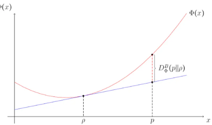
Figure 3.1: Illustration of the Bregman divergenceDBΦ(p||ρ)as a vertical distance between
pand the tangential hyperplane to the graph ofΦat pointρtakingpandρas points in a
functional space.
3.2
Bregman Divergences
3.2.1
General Definition and Fundamental Properties
Bregman divergences are defined by convex functions Φ(the so-calledgenerating
function) in the following way using an functional interpretation (Bregman 1967, Frigyik et al. 2008b): LetΦbe a strictly convex real-valued function with the domain
L(the Lebesgue-integrable functions). Further,Φis assumed to be twice continu-ously Fr´echet-differentiable (Kantorowitsch and Akilow 1978). A Bregman diver-genceDBΦ :L × L −→R+is defined as
DBΦ(p||ρ) = Φ (p)−Φ (ρ)−δΦ (ρ)
δρ [p−ρ] (3.2)
where δΦ(δρρ) is the Fr´echet-derivative of the generating functionΦwith respect toρ
(see Sec. 4.1).
The Bregman divergenceDΦB(p||ρ)can be interpreted as a measure of convexity of thegeneratingfunctionΦ. Takingpandρas points in a functional spaceDB
Φ(p||ρ) plays the role of the vertical distance betweenpand the tangential hyperplane to the graph ofΦat pointρ, which is illustrated in Fig. 3.1.
According to (Cichocki et al. 2009, Frigyik et al. 2008b, Frigyik et al. 2008a, Santos-Rodr´ıguez et al. 2009, Banerjee et al. 2005, Boissonnat et al. 2007), well known fundamental properties of the Bregman divergence are:
Convexity A Bregman divergence is always convex in its first argument but not necessarily in its second argument.
Non-negativity DΦB(p||ρ)≥0andDΦB(p||ρ) = 0iffp≡ρ.
Asymmetry The Bregman divergence is not a metric (the triangle inequality does not hold in general) and usually is not symmetric:
DΦB(p||ρ)=6 DΦB(ρ||p).
DBΦ(p||ρ) is symmetric if and only if the Hessian δ2δpΦ(2p) is constant on L
(Boissonnat et al. 2007).
Symmetrization For non-symmetric Bregman divergenceDBΦ, the symmetrized di-vergence is defined via
DB,symΦ (p||ρ) =DB,symΦ (ρ||p) = 1 2 D B Φ(p||ρ) +DBΦ(ρ||p) .
Linearity Bregman divergences are linear according to the generating functionΦ:
DBΦ 1+λΦ2(p||ρ) =D B Φ1(p||ρ) +λ·D B Φ2(p||ρ), λ >0.
Invariance A Bregman divergence is invariant under affine transformations. Thus,
DBΓ (p||ρ) =DΦB(p||ρ)
is valid for any affine transformation
Γ (ρ) = Φ (ρ) + Ψp[ρ] +ξ
with linear operator
Ψp[ρ] =
δΓ (p)
δp [ρ]− δΦ (p)
δp [ρ]
for positive measurespandρand scalarξ.
Three-point property For any triplep,ρ,τof positive measures the property
DBΦ(p||τ) =DΦB(p||ρ) +DΦB(ρ||τ) + δΦ (ρ) δρ [p−ρ]− δΦ (τ) δτ [p−ρ] holds.
Generalized Pythagorean theorem LetPΩ(ρ) = arg min
ω∈Ω
DΦB(ω||ρ)be the Bregman projection onto the convex setΩandp∈Ω. The inequality
DBΦ(p||ρ)≥DBΦ(p||PΩ(ρ)) +DBΦ(PΩ(ρ)||ρ)
is known as generalized the Pythagorean theorem. IfΩis an affine set it holds with equality.
Sensitivity The sensitivity of a Bregman divergence atpis defined as
s(p, τ) = ∂ 2DB Φ(p||p+ατ) ∂α2 α=0 (3.3) = −τδ 2Φ (p) δp2 τ
withτ ∈ Land the restriction thatR
τ(x)dx= 0. Note that δ2δpΦ(2p) is the
Hes-sian of the generating function. The sensitivitys(p, τ)measures the velocity of change of the divergence at the pointpin the direction ofτ.
Optimality Given a setS of positive measurespwith the (functional) mean µ =
E[S]andµ∈S. Then, for givenp∈S, the unique minimizer ofEp
DΦB(p||ρ)
isρ=µ. The inverse direction of this statement is also true: ifEp
DB
Φ(p||ρ)
is minimal forρ =µthenDB
Φ(p||ρ)is a Bregman divergence. This property predestinates Bregman divergences for clustering problems.
3.2.2
Bregman Geometry
In the following we will discuss some basic elements of Bregman geometry to clarify the basic geometric properties. Further, this will be useful to understand the behaviour of Bregman divergences for clustering. For a more detailed discus-sion of Bregman geometry we refer to Boissonnat et al. (2007) and Nielsen et al. (2005, 2006, 2009).
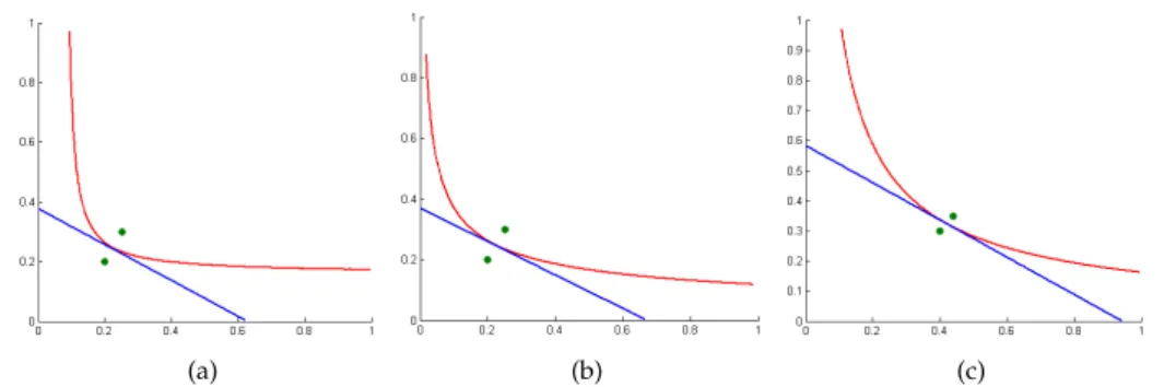
Bregman Bisectors
As mentioned above, Bregman divergences are not symmetric. Thus, we can define several types of bisectors. The Bregman bisector of thefirst typeis defined as
HΦ(p, ρ) ={τ ∈ L |DΦB(τ||p) =D
B
Φ(τ||ρ)} (3.4) and the Bregman bisector of thesecond typeis defined as
(a) (b) (c)
Figure 3.2: Bregman bisectors for arbitrarily chosen points in R2: (a)
Itakura-Saito-divergence, (b) and (c) generalized Kullback-Leibler-divergence. First-type bisectors are drawn in blue, second-type bisectors are drawn in red.
These bisectors are identical when the divergence is symmetric. However, in gen-eral, they are distinct. The bisectors of the first type are linear while the bisectors of the second type are potentially curved (but always linear in the gradient space) (Boissonnat et al. 2007). Obviously,pandρlie on different sides ofHΦ(p, ρ). Fig-ure 3.2 shows bisectors for some arbitrarily chosen points inR2for the Itakura-Saito
divergence (defined in (3.7)) and the (generalized) Kullback-Leibler divergence.
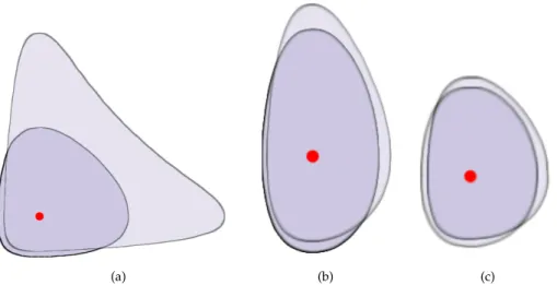
Bregman Balls and Bregman Spheres
Following the same argumentation as for Bregman bisectors, we can defineBregman
ballswith radiusr≥0of the first and the second types, depending on the argument
position of the centerc:
Bc,r = {τ ∈ L |DΦB(c||τ)≤r},
B0c,r = {τ ∈ L |DΦB(τ||c)≤r}.
Replacing the inequalities by equalities, we obtain the associated boundingBregman
spheres. The Bregman balls of the first type are convex while this is not necessarily
true for the balls of the second type (Boissonnat et al. 2007) as it is exemplarily shown for the Itakura-Saito divergence and the (generalized) Kullback-Leibler divergence in Fig. 3.3. Note that Bregman balls are not invariant by translation (Nielsen and Nock 2006), as illustrated in Fig. 3.3 (a) and (b) using the example of Itakuta-Saito divergence for two arbitrarily chosen distinct centers.
(a) (b) (c)
Figure 3.3: Examples of Bregman balls for arbitrarily chosen points inR2: Superposition of
the first typeBc,rand the second typeBc,r0 with the same center (red dot) and the same radius.
(a) and (b) Itakura-Saito-divergence, (c) generalized Kullback-Leibler-divergence.
3.2.3
Important Representatives of Bregman Divergence
The class of Bregman divergences includes many prominent dissimilarity measures. In the following we give some important examples. We may remark again that all these divergences can be defined via (3.2) using the respective generating function. Generalized Kullback-Leibler-Divergence
Thegeneralized Kullback-Leibler-divergencefor non-normalizedpandρis defined as
(Cichocki et al. 2009): DGKL(p||ρ) = Z plog p ρ dx− Z (p−ρ)dx (3.6) with the generating function
Φ (f) = Z
(f·logf−f)dx .
Ifpandρare normalized densities (probability densities)DGKL(p||ρ)is reduced to
the usual Kullback-Leibler-divergence (2.6) (Kullback and Leibler 1951):
DKL(p||ρ) = Z plog p ρ dx ,
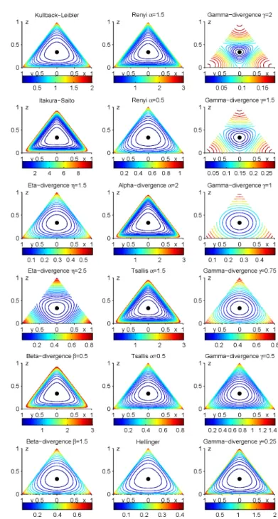
which is related to theShannon-entropyas stated in Eq. (2.7). Equidistance contours for three-dimensional probability densities using Kullback-Leibler divergence with respect to different reference points are displayed in the first row of Fig. 3.4 and 3.5. Itakura-Saito-Divergence
TheItakura-Saito-divergence (Itakura and Saito 1968)
DIS(p||ρ) = Z p ρ−log p ρ −1 dx (3.7)
is based on theBurg entropy(2.19) which also serves as the generating function
Φ (f) =HB(f) .
The Itakura-Saito-divergence is also known as negativecross Burg entropyand fulfills
thescale–property, that is
DIS(c·p||c·ρ) =DIS(p||ρ).
So the same relative weight is given to low and high energy components of p
(Bertin et al. 2009). Due to this, the Itakura-Saito-divergence was originally pre-sented as a measure of the quality of fits between two spectra and is frequently applied in image processing, sound processing, and speech processing (Nielsen and Nock 2007, F´evotte et al. 2009, Cont 2008).
Euclidean Distance
The Euclidean distance in terms of a Bregman-divergence is obtained by the gener-ating function
Φ (f) = Z
f2dx
We extend this definition and introduce the parametrized version
Φη(f) =
Z
fηdx
defining theη−divergencealso to be known as norm-like divergence (Nielsen and Nock 2009):
DE(p||ρ) =
Z
pη+ (η−1)·ρη−η·p·ρ(η−1)dx, (3.8) which obviously is the Euclidean distance for η = 2. To ensure the convexity of
β-Divergences
For positive measurespandρ, an important subset of Bregman divergences belong to the class ofβ-divergences(Eguchi and Kano 2001), which are defined, following Cichocki et al. (2009), as DB(p||ρ) = Z p·p β−1−ρβ−1 β−1 dx− Z pβ−ρβ β dx (3.9) = Z pβ 1 β−1 − 1 β −ρβ−1 p β−1− ρ β dx (3.10) withβ6= 1andβ 6= 0with the generating function
Φ (f) = f
β−β·f+β−1
β(β−1) .
In the limit β → 1 the divergence DB(p, ρ) becomes the generalized
Kullback-Leibler-divergence (3.6)1. The limitβ →0gives the Itakura-Saito-divergence (3.7).
Further,β−divergences are equivalent to the density power divergencesDˆB
intro-duced in (Basu et al. 1998) by
ˆ
DB(p||ρ) =
1
(1 +β)DB(p||ρ) .
Obviously,η−divergence (3.8) is a rescaled version ofβ−divergence forη=β:
DE(p||ρ) =β·(β−1)·DB(p||ρ) .
Thus, we see that forβ = 2theβ−divergenceDB(p||ρ)becomes (half) the Euclidean
distance.
3.3
Csisz´ar’s
f
-Divergences
3.3.1
General Definition and Fundamental Properties
Csisz´ar’sf-divergences are connected with the “ratio test” in the Pearson-Neyman style hypothesis testing and are in many ways “natural” concerning distributions and statistics (Cover and Thomas 2006). We denote byF the class of convex, real-valued, continuous functionsf satisfyingf(1) = 0, with
F={f|f : [0,∞)→R, f- convex} .
1We remark here that the relationspγ−ργ
γ γ−→→0log
p
ρand
pγ−1
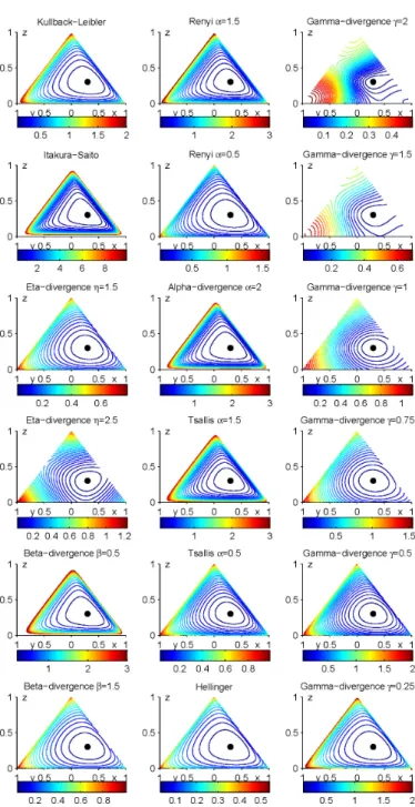
Figure 3.4: Equidistance levels of some example divergences for probability densities with
respect to reference point(0.3,0.3,0.3). The columns show Bregman divergences, Csisz´ar-f
Figure 3.5:The same as Fig. 3.4, but with another reference point: Equidistance levels of some
example divergences for probability densities with respect to reference point(0.5,0.2,0.3).
The columns show Bregman divergences, Csisz´ar-f divergences and Gamma divergences, respectively.
For a functionf ∈ Fthef-divergencesDf for positive measurespandρis given by Df(p||ρ) = Z ρ·f p ρ dx (3.11)
with the definitions0·f 0 0 = 0,0·f a 0 = limx→0x·f ax = limu→∞a· f(uu) (Csisz´ar 1967, Liese and Vajda 2006, Taneja and Kumar 2004). The function f is calleddetermining functionforDf(p||ρ). Csisz´ar’sf-divergences are related to the
generalizedf-entropy (Eq. (2.21)) via
Hf(p) =−Df(p||I)
withI being the constant function of value1 (Cichocki and Amari 2010). Thef -divergenceDf can be interpreted as an average of the likelihood ratiopρ describing
the change rate ofpwith respect toρweighted by the determining functionf. Some basic properties of thef-divergences are ( ¨Osterreicher 2002, Cichocki et al. 2009, Liese and Vajda 1987):
Non-negativity For probability density functionsp, ρ it holdsDf(p||ρ) ≥ 0. The
equal sign holds iffp≡ρ, which follows from the Jensen’s inequality. Convexity Df(p||ρ)is jointly convex in both argumentspandρ.
Scalability For any positive constantc >0it holds thatcDf(p||ρ) =Dcf(p||ρ).
Invariance The determining functionf defines an equivalence class in the sense thatDf(p||ρ) = Dfˆ(p||ρ)ifff(x) = ˆf(x) +c·(x−1) for densitiesp, ρand
c∈R, i.e.Df(p||ρ)is invariant according to a linear shift regarding the
deter-mining functionf.
Symmetry Letf, f∗∈ F, wheref∗is theconjugate functionoff, i.e.f∗(x) =x·f 1x forx∈(0,∞). Then the relationDf(p||ρ) = Df∗(ρ||p)is valid iff there exists
ac∈Rsuch thatf(x) =f∗(x) +c·(x−1)(i. e. the conjugate differs from the
original by a linear shift as above). A symmetric divergence can be obtained for an arbitrary convex functiong∈ Fusing its conjugateg∗for the definition
f =g+g∗as determining function. Upper bound Thef-divergence is bounded by
Df(p||ρ)≤ lim
u→0+{f(u) +f
∗(u)} .
(3.12) The existence of this limit for probability densitiespandρwas shown by Liese and Vajda (Liese and Vajda 1987). However, we state the following lemma:
Lemma 1. Letpandρbe positive measures. Then the bound given in (3.12) is still valid.
Proof.The proof is given in Appendix A.
Monotonicity The f-divergence is monotonic with respect to the coarse-graining of the underlying domainDof the positive measurespandρ, which is sim-ilarly to the monotonicity of the Fisher metric (Amari and Nagaoka 2000): Let K={κ(y|x)≥0, x∈D, y∈Dy} withDy being the range ofy. κdescribes
a transition probability density, i. e.R
κ(y|x)dy=1holds∀x∈ D. Denoting the positive measures ofy derived fromp(x)and ρ(x)bypκ(y)and ρκ(y)the
monotonicity is expressed byDf(p||ρ)≥Df(pκ||ρκ).2
Isomorphism Let
h:x7−→y (3.13)
be an invertible function transforming positive measuresp1(x)andρ1(x)to
p2(y)and ρ2(y). ThenDf(p1||ρ1) = Df(p2||ρ2)holds and the pairs(p1, ρ1) and(p2, ρ2)are called isomorph (Liese and Vajda 1987). Conversely, if a mea-sureD(p||ρ) =R
ρ(x)·G(p(x), ρ(x))dxfor an integrable functionGis invari-ant according to invertible transformationsh, thenD is af-divergence (Qiao and Minematsu 2008).
This isomorphism as well as the monotonicity suggest f-divergences for ap-plication in speech, signal and pattern recognition (Basseville 1989, Qiao and Minematsu 2008).
For a general f, not necessarily being convex, a generalization of the f -divergencesDfwas proposed by Cichocki et al. (2009):
DGf (p||ρ) =cf Z (p−ρ)dx+ Z ρ·f p ρ dx (3.14)
withcf = f0(1) 6= 0and denoted asgeneralizedf-divergence. As a consequence
of this relaxation of the convexity condition, in case ofpand ρbeing probability densities, the first term of (3.14) vanishes, such that the usual form off-divergences is obtained.
3.3.2
Important Representatives of
f
-Divergence
Some well-known examples off-divergences are given in the following. In order to illustrate the behaviour of differentf-divergences, Fig. 3.4 and 3.5 display the contours of equal divergence in the simplex (compare to Fig. 2.4) for several f -divergences (among others).
2The equality holds iff the conditional densitiespκ(x|y) =p(x)·κ(y|x)
pκ(y) andρκ(x|y) =
ρ(x)·κ(y|x)
ρκ(y) are
α-Divergences
As theβ−divergences in case of Bregman divergences, one can identify an impor-tant subset of thef−divergences, the so-calledα-divergences according to the defi-nition given in (Cichocki et al. 2009):
DA(p||ρ) = 1 α(α−1) Z pαρ1−α−α·p+ (α−1)ρdx (3.15) = 1 α(α−1) Z ρ p ρ α + (α−1) −α·p dx (3.16)
with the generatingf−function
f(u) =u u
α−1−1
α2−α + 1−u
α
and u = ρp and α > 0. In the limit α → 1 the generalized Kullback-Leibler-divergenceDGKL(3.6) is obtained. The caseα= 12is known as Hellinger divergence (see Eq. (3.23)). Changingαto1−αswaps the position ofpandρ(Minka 2005). Consequently, forα→0, we obtain the reverse KullbackLeibler divergence:
lim
α→0DA(p||ρ) =DGKL(ρ||p).
Further, in (Cichocki et al. 2009) is stated that theβ-divergences can be generated from theα-divergences applying the non-linear transforms
p→pβ+2andρ→ρβ+2withα= 1
β+ 1.
In addition to the general properties of thef−divergences stated above, one can de-rive an characteristic behaviour for theα-divergences directly from (3.15) depend-ing on the choice of the parameterα(Minka 2005): Forα0the minimization of
DA(p||ρ)to estimateρ(x)may exclude modes of the targetp(x), or more
specifi-cally: The best approximation may represent only one mode, the one with largest mass (not the mode which is highest peak). Further, forα≤ 0theα-divergence is zero-forcing, i.e.,p(x) = 0forcesρ(x) = 0, while forα≥1it is zero-avoiding, that isρ(x)>0wheneverp(x) >0.Forα→ ∞,ρ(x)coversp(x)completely and the
α-divergence is called inclusive in that case.
It is important to note, that the α-divergence is a continuous function of real variableαfor the whole range including singularities (Cichocki and Amari 2010).
Tsallis Divergence
TheTsallis-divergenceis a widely applied divergence related toα-divergence (3.15),
however, only defined for probability densities. It is defined as
DTA(p||ρ) =− Z p·logα ρ p dx (3.17)
with the convention
logα(z) = z 1−α−1 1−α such that DTA(p||ρ) = 1 1−α 1− Z pαρ1−αdx (3.18) andα 6= 1. Obviously, this is a rescaled version of theα-divergence (3.15), which only holds for probability densities (Cichocki and Amari 2010):
DTA(p||ρ) =α·DA(p||ρ). (3.19)
The Tsallis-divergence is based on the Tsallis-entropy (2.17). In the limitα→1the divergenceDT
A(p||ρ)converges to the Kullback-Leibler-divergence (2.6).
Generalized R´enyi-Divergences
Another family of divergences, closely related to theα−divergences, are the gener-alizedR´enyi-divergencesdefined as (Amari 1985, Cichocki et al. 2009):
DGRA (p||ρ) = 1 α−1log Z pαρ1−α−α·p+ (α−1)ρdx+ 1 (3.20) for positive measuresρandp. The generalized R´enyi-divergence can be written in terms of theα-divergence3
DGRA (p||ρ) = 1
α−1log (1 +α·(α−1)·DA(p||ρ)). (3.21)
For probability densities DGRA (p||ρ) reduces to the usual R´enyi-divergence (R´enyi 1961, R´enyi 1970): DAR(p||ρ) = 1 α−1log Z pαρ1−αdx . (3.22)
The divergenceDAR(p||ρ)is based on theR´enyi-entropy(2.12) via (3.35) as we will discuss in Sec. 3.6.
3Note that a careful transformation of the parameterαis required for exact transformations between
both divergences. For details see (Amari 1985, pp. 84ff) and (Cichocki et al. 2009, p. 104). Further, it should be mentioned here that this statement was given in this book without proving the bounds of the
Hellinger Divergence
Anotherf-divergence which is only properly defined for probability densitiespand
ρ, is theHellinger divergence(Liese and Vajda 2006, Taneja and Kumar 2004):
DH(p||ρ) =
1 2 Z
(√p−√ρ)2dx (3.23) with the generating functionf(u) = 2 (1−√u)foru= pρ.
3.4
γ
-Divergences
A class of very robust divergences with respect to outliers has been proposed by Fujisawa and Eguchi (2008). It is calledγ-divergencesdefined for positive measures
ρandpas DG(p||ρ) = log R pγ+1dxγ(γ1+1)· R ργ+1dxγ+11 R p·ργdxγ1 (3.24) = 1 γ+ 1log " Z pγ+1dx γ1 · Z ργ+1dx # (3.25) −log "Z p·ργdx γ1# .
It is proposed to be robust forγ∈[0,1]with existence ofDG in the limitγ →0. A
detailed analysis of robustness is given in (Fujisawa and Eguchi 2008).
In the limitγ→0DG(ρ||p)becomes the usual Kullback-Leibler-divergence (2.6)
DKL( ˆρ||pˆ)with normalized densities
ˆ
ρ= ρ
W(ρ)andpˆ=
p W(p) .
Forγ= 1theγ-divergence becomes theCauchy-Schwarz-divergence
DCS(p||ρ) = 1 2log Z ρ2dx· Z p2dx −log (V (p, ρ)) (3.26) with V(p, ρ) = Z p·ρdx (3.27)
being thecross correlation potential. TheCauchy-Schwarz-divergenceDCS(p||ρ)was
norms. It is based on the quadratic R´enyi-entropyH2R(p)from (2.12) (Jenssen 2005). Obviously,DCS(p||ρ)is symmetric. It is frequently applied for Parzen window
es-timation and particularly suitable for spectral clustering as well as for related graph cut problems (Jenssen 2005, Jenssen et al. 2006, Principe et al. 2000).
The most important properties of theγ-divergence are the following:
Invariance The divergenceDG(p||ρ)is invariant under scalar multiplication with
positive constantsc1andc2:
DG(p||ρ) =DG(c1·p||c2·ρ) .
In case of positive measures the equationDG(p||ρ) = 0holds only ifp=c·ρ
withc >0. For probability densitiesc= 1is required.
Isomorphism Theγ-divergence is not invariant with respect toh-transformations (3.13), but affine invariant, i. e. similar tof-divergences, here an isomorphism can be stated forh-transformations, which, more strictly, have to be affine. Pythagorean relation As for Bregman divergences a modified Pythagorean relation
between positive measures can be stated for special choices ofp,ρ,τ: Letpε
be a distortion ofρdefined as convex combination with a positive distortion measureδrelated to outlieres:
pε(x) = (1−ε)·ρ(x) +ε·δ(x) .
Further a positive measuregis defined to beδ-consistentif
νg=
Z
δ(x)g(x)αdx
α1
is sufficiently small for largeα > 0, i. e. the bias caused by outliers can be neglected. This implies that the contamination densityδ(x)mostly lies on the tail of the underlying density g(x). If two positive measuresρandτ are δ -consistent according to a distortion measureδ, then the Pythagorean relation approximately holds forρ,τand the distortionpεofρ
DG(pε||τ)−DG(pε||ρ)−DG(ρ||τ) =O(ενγ)
withν = max{νρ, ντ}. This property implies the robustness ofγ-divergences
with respect to distortions according to the resulting approximation
DG(pε||τ)≈DG(pε||ρ) +DG(ρ||τ)
andDG(pε||ρ)should be small becausepεis assumed to be a distortion ofρ
Some equidistance contours for three-dimensional probability densities using the
γ-divergence and different values ofγare shown in the last column of Fig. 3.4 and 3.5.
In (Cichocki and Amari 2010) it was shown that the whole family of γ -divergences can be generated directly fromα-divergences and alsoβ-divergences.
3.5
Metric Divergences
Generally, divergences are measures of dissimilarity but not symmetric and, there-fore, cannot serve as a metric (Cichocki and Amari 2010, Cichocki et al. 2011, Gretton et al. 2005). If a function of the divergence is a metric, then it becomes much more powerful (Chen et al. 2008b). However, the most critical property of a metricDis the triangle inequalityD(p||ρ)≤D(p||z) +D(z||ρ). This property has many appli-cations. For instance, the triangle inequality may save a lot of effort in finding the nearest neighbour in a multidimensional vector space (Chen et al. 2008a). In this section we will give some examples of metric divergences for densitiespandρ.
The most prominent distance belonging to the class of Bregman divergences is theEuclidean distancewhich is aη-divergence (3.8) with parameterη = 2(Nielsen and Nock 2009) as mentioned before.
Another representative of the class of Bregman divergences is the Jensen-Shannon divergence DJ S(p||ρ) = 1 2 DKL p||p+ρ 2 +DKL ρ||p+ρ 2 , (3.28) whereDKLis the Kullback-Leibler divergence (2.6). It can be calculated based on
the Shannon entropyH(p)(2.5) as
DJ S(p||ρ) =H p+ρ 2 − H(p) +H(ρ) 2 (3.29) as shown in (Shannon and Weaver 1949). It has been proved in (Endres and Schindelin 2003), that the square root of the Jensen-Shannon divergence (3.28) p
DJ S(p||ρ)is a metric. Moreover, it is always finite for any two densities. However,
Jensen-Shannon divergence is simply an averaged Bregman divergence associated with the convex functionxlogx(Chen et al. 2008a). Generally, Chen et al. (2008a) provide necessary and sufficient conditions for a convex function so that thesquare root of its associated average Bregman divergenceis a metric. In the second part of their paper, Chen et al. provide amin−maxapproach to get a metric from a Bregman divergence (Chen et al. 2008b).