Politecnico di Torino
Porto Institutional Repository
[Proceeding] PaMPa-HD: A Parallel MapReduce-Based Frequent Pattern
Miner for High-Dimensional Data
Original Citation:
Apiletti, D.; Baralis, E.; Cerquitelli, T.; Garza, P.; Michiardi, P.; Pulvirenti, F. (2015).
PaMPa-HD:
A Parallel MapReduce-Based Frequent Pattern Miner for High-Dimensional Data.
In: The 3rd
International Workshop on High Dimensional Data Mining (HDM’15), Atlantic City, NJ, USA, 14
November 2015. pp. 839-846
Availability:
This version is available at :
http://porto.polito.it/2639879/
since: April 2016
Publisher:
IEEE
Published version:
DOI:
10.1109/ICDMW.2015.18
Terms of use:
This article is made available under terms and conditions applicable to Open Access Policy Article
("Public - All rights reserved") , as described at
http://porto.polito.it/terms_and_conditions.
html
Porto, the institutional repository of the Politecnico di Torino, is provided by the University Library
and the IT-Services. The aim is to enable open access to all the world. Please
share with us
how
this access benefits you. Your story matters.
PaMPa-HD: a Parallel MapReduce-based
frequent Pattern miner for High-Dimensional
data
Daniele Apiletti, Elena Baralis, Tania Cerquitelli,
Paolo Garza, and Fabio Pulvirenti Dipartimento di Automatica e Informatica
Politecnico di Torino
Torino, Italy
Email: [email protected] Pietro Michiardi Eurecom
Sophia Antipolis, France
Email: [email protected]
Abstract
Frequent closed itemset mining is among the most complex exploratory techniques in data mining, and provides the ability to discover hidden correlations in transactional datasets. The explosion of Big Data is leading to new parallel and distributed approaches. Unfortunately, most of them are designed to cope with low-dimensional datasets, whereas no distributed high-dimensional frequent closed itemset mining algorithms exists. This work introduces PaMPa-HD, a parallel MapReduce-based frequent closed itemset mining algorithm for high-dimensional datasets, based on Carpenter. The experimental results, performed on both real and synthetic datasets, show the efficiency and scalability of PaMPa-HD.
I. INTRODUCTION
In the last years, the increasing capabilities of recent applications to produce and store huge amounts of information, the so called ”Big Data”, have changed dramatically the importance of the intelligent analysis of data. In both academic and industrial domains, the interest towards data mining, which focuses on extracting effective and usable knowledge from large collections of data, has risen. The need for efficient and highly scalable data mining tools increases with the size of the datasets, as well as their value for businesses and researchers aiming at extracting meaningful insights increases.
Frequent (closed) itemset mining is among the most complex exploratory techniques in data mining. It is used to discover frequently co-occurring items according to a user-provided frequency threshold, called minimum support. Existing mining algorithms revealed to be very efficient on basic datasets but very resource intensive in Big Data contexts. In general, applying data mining techniques to Big Data collections has often entailed to cope with computational costs that represent a critical bottleneck. For this reason, we are witnessing the explosion of parallel
2
and distributed approaches, typically based on distributed frameworks, such as Apache Hadoop [1] and Spark [2]. Unfortunately, most of the scalable distributed techniques for frequent itemset mining have been designed to cope with datasets characterized by few items per transaction (low dimensionality, short transactions), focusing, on the contrary, on very large datasets in terms of number of transactions. Currently, only single-machine implementations exist to address very long transactions, such as Carpenter [3], and no distributed implementations at all.
Nevertheless, many researchers in scientific domains such as bioinformatics or networking, often require to deal with this type of data. For instance, most gene expression datasets are characterized by a huge number of items (related to tens of thousands of genes) and a few records (one transaction per patient or tissue). Many applications in computer vision deal with high-dimensional data, such as face recognition. Some smart-cities studies have built this type of large datasets measuring the occupancy of different car lanes: each transaction describes the occupancy rate in a captor location and in a given timestamp [4]. In the networking domain, instead, the heterogeneous environment provides many different datasets characterized by high-dimensional data, such as URL reputation, advertising, and social network datasets [4], [5].
This work introduces PaMPa-HD, a parallel MapReduce-based frequent closed itemset mining algorithm for high-dimensional datasets, based on the Carpenter algorithm. PaMPa-HD outperforms the single-machine Carpenter implementation and the best state-of-the-art distributed approaches, in both execution time and minimum support threshold. Furthermore, the implementation takes into account crucial design aspects, such as load balancing and robustness to memory-issues.
The paper is organized as follows: Section II introduces the frequent (closed) itemset mining problem, Section III briefly describes the centralized version of Carpenter, and Section IV presents the proposed PaMPa-HD algorithm. Section V describes the experimental evaluations proving the effectiveness of the proposed technique, Section VI provides a brief review of the state of the art, and Section VII discusses possible applications of PaMPa-HD. Finally, Section VIII introduces future works and conclusions.
II. FREQUENT ITEMSET MINING BACKGROUND
Let I be a set of items. A transactional dataset D consists of a set of transactions {t1, . . . , tn}, where each
transaction ti ∈ D is a set of items (i.e., ti ⊆ I) and it is identified by a transaction identifier (tidi). Figure 1a
reports an example of a transactional dataset with 5 transactions. The dataset reported in Figure 1a is used as a running example through the paper.
An itemset I is defined as a set of items (i.e., I ⊆ I) and it is characterized by a tidlist and a support value. The tidlist of an itemsetI, denoted bytidlist(I), is defined as the set of tids of the transactions in Dcontaining
I, while the support ofI in D, denoted bysup(I), is defined as the ratio between the number of transactions in
D containingI and the total number of transactions inD (i.e., |tidlist(I)|/|D|). For instance, the support of the itemset{aco} in the running example datasetDis 2/5 and its tidlist is{1,3}. An itemsetI is considered frequent if its support is greater than a user-provided minimum support thresholdminsup.
Given a transactional dataset D and a minimum support threshold minsup, the Frequent Itemset Mining [6] problem consists in extracting the complete set of frequent itemsets from D. In this paper, we focus on a valu-able subset of frequent itemsets called frequent closed itemsets [3]. Closed itemsets allow representing the same information of traditional frequent itemsets in a more compact form.
D tid items 1 a,b,c,l,o,s,v 2 a,d,e,h,l,p,r,v 3 a,c,e,h,o,q,t,v 4 a,e,f,h,p,r,v 5 a,b,d,f,g,l,q,s,t
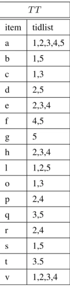
(a) Horizontal representation ofD T T item tidlist a 1,2,3,4,5 b 1,5 c 1,3 d 2,5 e 2,3,4 f 4,5 g 5 h 2,3,4 l 1,2,5 o 1,3 p 2,4 q 3,5 r 2,4 s 1,5 t 3.5 v 1,2,3,4 (b) Transposed represen-tation ofD T T|{2,3} item tidlist a 4,5 e 4 h 4 v 4 (c) T T|{2,3}: ex-ample of conditional transposed table
Fig. 1. Running example datasetD
A transactional dataset can also be represented in a vertical format, which is usually a more effective representation of the dataset when the average number of items per transactions is orders of magnitudes larger than the number of transactions. In this representation, also called transposed tableT T, each row consists of an itemi and its list of transactions, i.e.,tidlist({i}). Letr be an arbitrary row ofT T,r.tidlistdenotes the tidlist of rowr. Figure 1b reports the transposed representation of the running example reported in Figure 1a.
Given a transposed tableT T and a tidlistX, the conditional transposed table ofT T on the tidlistX, denoted by
T T|X, is defined as a transposed table such that: (1) for each rowri ∈T T such thatX ⊆ri.tidlistthere exists
one tupler0i∈T T|X and (2) ri0 contains all tids inri.tidlistwhose tid is higher than any tid in X.
For instance, consider the transposed tableT T reported in Figure 1b. The projection ofT T on the tidlist{2,3}
is the transposed table reported in Figure 1c.
Each transposed table T T|X is associated with an itemset composed by the items in T T|X. For instance, the
4
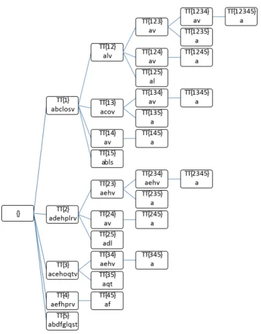
Fig. 2. The transaction enumeration tree of the running example dataset in Figure 1a. For the sake of clarity, no pruning rules are applied to the tree.
III. THECARPENTER ALGORITHM
As discussed in section VI, the most popular techniques (e.g., Apriori and FP-growth) adopt the itemset enumer-ation approach to mine the frequent itemsets. However, itemset enumerenumer-ation revealed to be ineffective with datasets with a high average number of items per transactions [3]. To tackle this problem, the Carpenter algorithm [3] was proposed. Specifically, Carpenter is a frequent itemset extraction algorithm devised to handle datasets characterized by a relatively small number of transactions but a huge number of items per transaction. To efficiently solve the itemset mining problem, Carpenter adopts an effective depth-first transaction enumeration approach based on the transposed representation of the input dataset. To illustrate the centralized version of Carpenter, we will use the running example datasetDreported in Figure 1a, and more specifically, its transposed version (see Figure 1b). As already described in Section II, in the transposed representation each row of the table consists of an itemiwith its tidlist. For instance, the last row of Figure 1b points that item vappears in transactions 1, 2, 3, 4.
Carpenter builds a transaction enumeration tree where each node corresponds to a conditional transposed table
T T|X and its related information (i.e., the tidlistX with respect to which the conditional transposed table is built
and its associated itemset). The transaction enumeration tree, when pruning techniques are not applied, contains all the tid combinations (i.e., all the possible tidlistsX). Figure 2 reports the transaction enumeration tree obtained by processing the running example dataset. To avoid the generation of duplicate tidlists, the transaction enumeration tree is built by exploring the tids in lexicographical order (e.g.,T T|{1,2} is generated instead of T T|{2,1}). Each
node of the tree is associated with a conditional transposed table on a tidlist. For instance, the conditional transposed tableT T|{2,3} in Figure 1c, matches the node{2,3} in Figure 2.
Carpenter performs a depth first search of the enumeration tree to mine the set of frequent closed itemsets. Referring to the tree in Figure 2, the depth first search would lead to the visit of the nodes in the following order: {1}, {1,2}, {1,2,3}, {1,2,3,4}, {1,2,3,4,5}, {1,2,3,5}, {...}. For each node, Carpenter applies a procedure that decides if the itemset associated with that node is a frequent closed itemset or not. Specifically, for each node, Carpenter decides if the itemset associated with the current node is a frequent closed itemset by considering: 1) the tidlistX associated with the node, 2) the conditional transposed tableT T|X, 3) the set of frequent closed itemsets
found up to the current step of the tree search, and 4) the enforced minimum support threshold (minsup). Based on the theorems reported in [3], if the itemsetIassociated with the current node is a frequent closed itemset thenI
is included in the frequent closed itemset set. Moreover, by exploiting the analysis performed on the current node, part of the remaining search space (i.e., part of the enumeration tree) can be pruned, to avoid the analysis of nodes that will never generate new closed itemsets. At this purpose, three pruning rules are applied on the enumeration tree, based on the evaluation performed on the current node and the associated transposed tableT T|X:
• Pruning rule 1. If the size of X, plus the number of distinct tids in the rows of T T|X does not reach the
minimum support threshold, the subtree rooted in the current node is pruned.
• Pruning rule 2.If there is any tidtidi that is present in all the tidlists of the rows ofT T|X,tidi is deleted
fromT T|X. The number of discarded tids is updated to compute the correct support of the itemset associated
with the pruned version of T T|X.
• Pruning rule 3. If the itemset associated with the current node has been already encountered during the depth first search, the subtree rooted in the current node is pruned because it can never generate new closed itemsets.
The tree search continues in a depth first fashion moving on the next node of the enumeration tree. More specifically, let tidl be the lowest tid in the tidlists of the current T T|X, the next node to explore is the one
associated withX0=X∪ {tidl}.
Among the three rules mentioned above, pruning rule 3 assumes a global knowledge of the enumeration tree explored in a depth first manner. This, as detailed in section IV, is very challenging in a distributed environment.
IV. THEPAMPA-HDALGORITHM
Given the complete enumeration tree (see Figure 2), the centralized Carpenter algorithm extracts the whole set of closed itemsets by performing a depth first search (DFS) of the tree. Carpenter also prunes part of the search space by applying the three pruning rules illustrated above. The PaMPa-HD algorithm proposed in this paper splits the depth first search process in a set of (partially) independent sub-processes, that autonomously evaluate sub-trees of
6
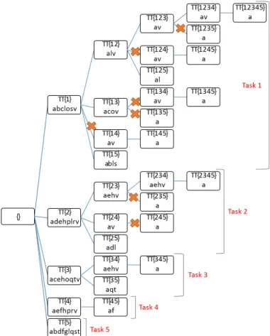
Fig. 3. Running toy example: each node expands a branch of the tree independently. Pruning rule 1 and 2 are not applied. The pruning rule 3 is applied only within the same task: the crosses on the edges represent pruned nodes due to local pruning rule 3.
the search space. Specifically, the whole problem can be split by assigning each subtree rooted inT T|X, whereX is
a single transaction id in the initial dataset, to an independent sub-process. Each sub-process applies the centralized version of Carpenter on its conditional transposed tableT T|Xand extracts a subset of the final closed itemsets. The
subsets of closed itemsets mined by each sub-processe are merged to compute the whole closed itemset result. Since the sub-processes are independent, they can be executed in parallel by means of a distributed computing platform, e.g., Hadoop. Figure 3 shows the application of the proposed approach on the running example. Specifically, five independent sub-processes are executed in the case of the running example, one for each row (transaction) of the original dataset.
Partitioning the enumeration tree in sub-trees allows processing bigger enumeration trees with respect to the centralized version. However, this approach does not allow fully exploiting pruning rule 3 because each sub-process works independently and is not aware of the partial results (i.e., closed itemsets) already extracted by the other
sub-processes. Hence, each sub-process can only prune part of its own search space by exploiting its “local” closed itemset list, while it cannot exploit the closed itemsets already mined by the other sub-processes. For instance, Task T2 in Figure 3 extracts the closed itemset av associated with node T T|2,4. However, the same closed itemset is
also mined by T1 while evaluating node T T|1,2,3,4. In the centralized version of Carpenter, the duplicate version
of av associated with node T T|2,4 is not generated because T T|2,4 follows T T|1,2,3,4 in the depth first search,
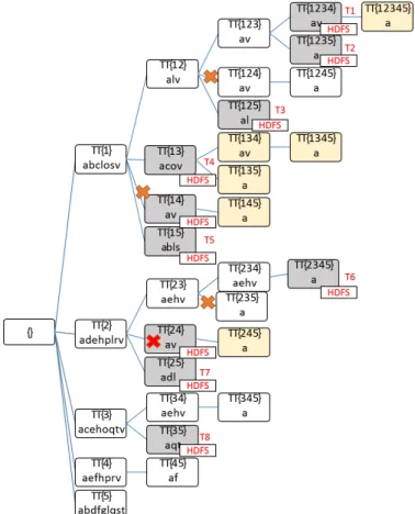
i.e., the tasks are serialized and not parallel. Since pruning rule 3 has a high impact of the reduction of the search space, its inapplicability leads to a negative impact on the execution time of the distributed algorithm as described so far. To address this issue, we share partial results among the sub-processes. Each sub-process analyzes only a part the search subspace, then, when memory is full or when a maximum number of visited nodes is reached, it stores on disk (e.g., in HDFS, the Hadoop distributed file system) the partial set of closed itemset mined so far and the remaining sub-tree left to analyze. A synchronization and pruning task works on the partial results of the sub-processes to globally apply pruning rule 3 on the remaining search subspaces, i.e., on the remaining nodes of the enumeration tree. After the application of the synchronization and pruning step, a new set of sub-processes is defined, for each remaining node of the enumeration tree. The overall process is applied iteratively by instantiating new sub-processes and synchronizing their results, until there are no nodes left.
The application of this approach to our running example is represented in Figure 4. The table related to the itemset av associated with the tidlist/node{2, 4} is pruned because the synchronization job discovers a previous table with the same itemset, i.e. the node associated with the transaction ids combination{1, 2, 3, 4}. The use of this approach allows the parallel execution of the mining process, providing at the same time a very high reliability dealing with heavy enumeration trees, which can be split and pruned according to pruning rule 3.
A. Implementation details
PaMPa-HD implementation exploits Hadoop MapReduce. The algorithm consists of three MapReduce jobs. Job #1 reads the input dataset, in the transposed format, and builds the initial conditional transposed tables
T T|X, one for each tid (transaction id). The last step of the reducer locally runs the centralized Carpenter on each
conditional transposed table T T|X, until there is enough memory available and the number of processed nodes
of the enumeration tree rooted inT T|X is lower than a maximum number of iterations (the maximum expansion
threshold parameter of PaMPa-HD). If any of the two conditions is verified, the job ends by storing the currently-extracted frequent closed itemsets on disk (in HDFS [1]) along with the pointer to the next node of the enumeration tree to be processed, i.e., the next conditional T T|X.
Job #2 globally synchronizes the partial closed itemset lists and the intermediate conditional transposed tables saved on disk by job #1, by applying pruning rule 3.
Job #3 performs the same operations as job #1, but it receives in input the remainingT T|X of the enumeration
tree, instead of building them from the input dataset.
Job #2 and job #3 are repeated until no conditional tables remain.
Thanks to the introduction of a global synchronization phase (job #2), the proposed PaMPa-HD approach is able to apply pruning rule 3 and handle high-dimensional datasets, otherwise not manageable due to memory issues.
8
Fig. 4. Execution of PaMPa-HD on the running example dataset. For sake of clarity, pruning rules 1 and 2 are not applied. The crosses on nodes represent that the nodes have been removed by the synchronization job, e.g., the one on node{2 4}represents the pruning of node{2 4}.
V. EXPERIMENTS
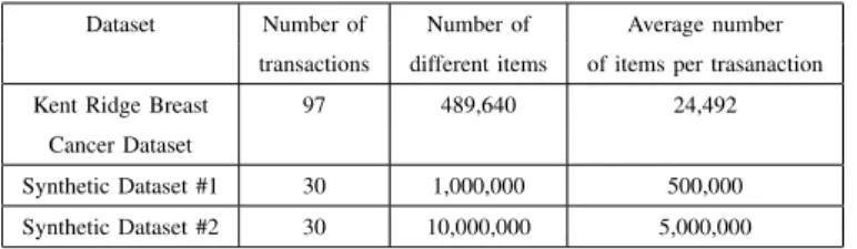
We performed a set of experiments to evaluate (i) the efficiency of the proposed algorithm in comparison with the state of the art approaches (Section V-A), (ii) the impact of the parameter setting (see Section V-B), and (iii) the scalability of the algorithm with respect to the number of reducers/parallel tasks (see Section V-C). We performed the experiments on a popular real dataset and on two synthetic datasets. The real dataset is the theKent Ridge Breast Cancer[7] and contains gene expression data. It is characterized by 97 rows that represent patient samples, and 24,482 attributes related to genes. Data have been discretized with an equal depth partitioning using 20 buckets (similarly to [3]). The other two datasets were synthetically generated and tuned to simulate use cases characterized by extremely high-dimensional data, i.e., with massive numbers of features. Both datasets consists of 30 transactions. Dataset #1 has 1,000,000 different items and an average transaction length of 500,000 items, while
1: procedure DISTRIBUTED CARPEN
-TER(minsup;initial T T)
2: Job 1 Mapper: process each row of TT and send it to reducers
3: Job 1 Reducer: aggregates T T|x and run
Local Carpenter until expansion threshold is reached or memory is not enough
4: Job 2 Mapper: process all the closed itemset or transposed tables from the previous job and send them to reducers
5: Job 2 Reducers: for each itemset belonging to
a table or a frequent closed, keep the eldest in a Depth First fashion
6: Job 3 Mapper: process eachT T|xfrom the
previous job and run Local Carpenter until expansion threshold is reached or memory is not enough
7: Repeat Job 2 and Job 3 until no more conditional tables need to be processed
8: end procedure
Fig. 5. Distributed Carpenter pseudo code
Dataset #2 is 10 times larger, with 10,000,000 different items and an average transaction length of 5,000,000 items (see Table I). The discretized version of the real dataset and the synthetic dataset generator are publicly available at http://dbdmg.polito.it/PaMPa-HD/.
TABLE I. DATASETS
Dataset Number of Number of Average number transactions different items of items per trasanaction Kent Ridge Breast 97 489,640 24,492
Cancer Dataset
Synthetic Dataset #1 30 1,000,000 500,000 Synthetic Dataset #2 30 10,000,000 5,000,000
PaMPa-HD is implemented in Java 1.7.0 60 using the Hadoop MR API. Experiments were performed on a cluster of 5 nodes running Cloudera Distribution of Apache Hadoop (CDH5.3.1). Each cluster node is a 2.67 GHz six-core Intel(R) Xeon(R) X5650 machine with 32 Gbyte of main memory running Ubuntu 12.04 server with the 3.5.0-23-generic kernel.
10
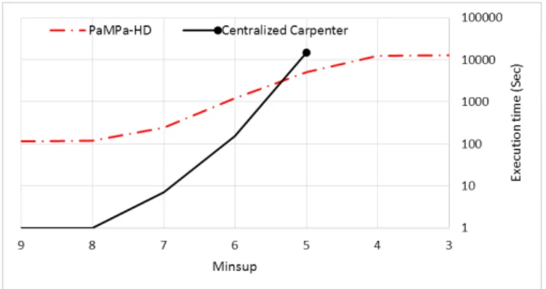
Fig. 6. Execution time for different Minsup values on the Breast Cancer real dataset.
A. Running time
In this section we analyze the efficiency of PaMPa-HD by comparison with two state-of-the-art algorithms: a main-memory centralized version of Carpenter, developed in C++ by Sam Borgelt [8], and a MapReduce-based implementation of FP-growth [9] available in Mahout 0.9 [10], (for details see Section VI). The comparison with Carpenter aims to show the ability of PaMPa-HD to address datasets that are not manageable by means of a centralized approach. The comparison with the Hadoop implementation of PFP is a reference benchmark since it represents the most scalable state-of-the-art approach for closed itemset mining, even if PFP was not specifically developed to deal with high-dimensional datasets as PaMPa-HD.
The first set of experiments has been performed with the Kent Ridge Breast Cancer dataset [7]. As reported in Figure 6 (Minsup axis is reversed to improve readability), the centralized version of Carpenter is faster than our approach with absolute minimum support thresholds (Minsup) of 6 or higher. However, when the search space to explore becomes larger (i.e., with low support minimum support thresholds) the centralized version is slower or runs out of memory (after days of processing), while PaMPa-HD is able to extract all the frequent closed itemsets. When the problem becomes more complex, and the size of the enumeration three increases, the advantages of the parallelization outperform the overheads of the distributed environment (e.g., communication and synchronization costs). Such overheads can be roughly estimated in the fixed 100 seconds time required by PaMPa-HD to be executed for high Minsup values (8 and 9 in Figure 6). The Hadoop PFP implementation reveals to be unsuitable for the extraction of frequent closed itmsets from the Kent Ridge Breast Cancer dataset: its execution time was more than one day of computation, even for the highest support threshold, so orders of magnitude higher than the others. For this reason, the execution time of PFP is not reported in Figure 6. This result highlights the need for specific algorithms particularly tailored to address high-dimensional data, such as PaMPa-HD, because traditional best-in-class approaches, such as PFP, cannot cope with the curse of dimensionality.
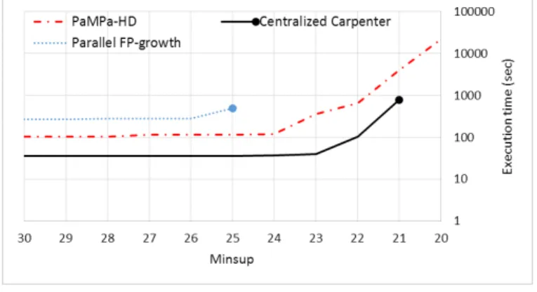
A second set of experiments using the synthetic Dataset #1 has been performed. In Dataset #1, even if the number of different items is only doubled with respect to the breast cancer dataset, the average number of items per transaction is much higher (one order of magnitude). This feature makes each conditional transposed table, associated with each node of the enumeration tree, much bigger and heavy to process. As reported in Figure 7, for very high Minsup values (20+) Carpenter scores the lowest execution times, with a Minsup value of 19 the
Fig. 7. Execution time for different Minsup values on synthetic Dataset #1.
Fig. 8. Execution time for different Minsup values on synthetic Dataset #2.
performance of PaMPa-HD and Carpenter are almost the same, but with Minsup values of 18 or lower, Carpenter runs out of memory and the task is unfeasible, whereas PaMPa-HD successfully completes the extraction. Furthermore, the time required for PaMPa-HD to complete the extraction in the latter case and its trend for decreasing Minsup values (19-18-17) is equal or less than the time required by PFP for respectively higher Minsup values (22-21-20). Not only PaMPa-HD is faster than PFP for high Minsup values (20+), but can it also scale further, since PFP stops at Minsup 20. The results prove that PaMPa-HD is effectively able to address problems that are unfeasible for both centralized state-of-the-art specialized techniques (Carpenter) and scalable state-of-the-art generic itemset mining algorithms (PFP).
The last set of performance experiments is executed on synthetic Dataset #2. Dataset #2 is extremely high-dimensional, achieving an average number of items per transaction of 5,000,000. The results, reported in Figure 8, confirm that (i) for high Minsup values (21+), the problem is conveniently solved by current specialized algorithms (Carpenter), (ii) both centralized algorithms and generic distributed approaches cannot cope with high-dimensional datasets with lower Minsup values, being 20 for Carpenter and 25 for PFP the lowest feasible Minsup values, ad (iii) the proposed PaMPa-HD algorithm provides both better execution times than PFP by almost an order of magnitude and higher scalability for more complex problems (lower Minsup values). Achieving lower Minsup values allows to discover deeply hidden knowledge, while high Minsup values usually lead to obvious information.
12
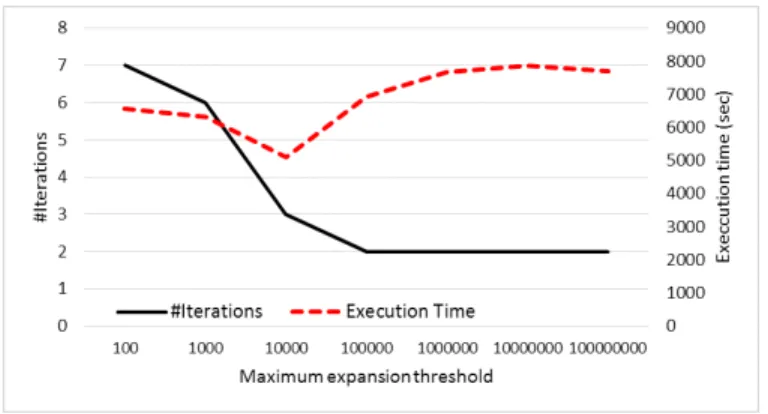
Fig. 9. Execution time and number of iterations for differentmax expvalues on Breast Cancer dataset withminsup=5.
B. Maximum expansion threshold
In this section we analyze the impact of the maximum expansion threshold (max exp) parameter, which indicates the maximum number of nodes to be explored before a preemptive stop of each distributed sub-process is forced. This parameter, as already discussed in Section IV, strongly affects the enumeration tree exploration, forcing each parallel task to stop before completing the visit of its sub-tree and write partial results on HDFS. This approach allows the synchronization job to globally apply pruning rule 3 and reduce the search space. Low values ofmax exp
threshold decrease the risks of memory issue, because the global problem is split into simpler and less memory-demanding sub-problems, and facilitate the application of pruning rule 3, hence a smaller subspace is searched. However, higher values allow a more efficient execution, by limiting the start and stop of distributed tasks (similarly to the context switch penalty), and the synchronization overheads.
This set of experiments has been performed on the Beast cancer dataset with Minsup 5, by varying max exp
from 100 to 100,000,000. Figure 9 shows the results in terms of execution time and number of iterations (i.e., the number of times the synchronization Job #2 is executed). The best performance in terms of execution time is achieved with a maximum expansion threshold equal to 10,000 nodes. With higher values, the number of iterations decreases, but more useless tree branches are explored, because pruning rule 3 is globally applied less frequently. Lower values ofmax exp, instead, introduce a performance degradation caused by the higher number of iterations and the synchronization phase overheads. With very high values ofmax exp, the running time and the number of iterations are stable because the bottleneck becomes the free available memory, and the synchronization job is automatically applied, independently of the value of max exp. The tuning of max exp is strictly related to the data distribution: in general, the easier the mining task, the fewer the benefits of having many iterations.
The value of max exp impacts also the load balancing of the distributed computation among different nodes. With low values of max exp, each task explores a smaller enumeration sub-tree, decreasing the size difference among the sub-trees analyzed by different tasks, thus improving the load balancing. Table II reports the minimum and the maximum execution time of the mining tasks executed in parallel for two extreme values of max exp. The load balance is better for the lowest value of max exp.
TABLE II. LOADBALANCING
Task execution time Maximum expansion threshold Min Max
100,000,000 4s 1h 54m 33s 100,000 4s 1h 2m 32s 10000 4s 23m 50s
100 4s 53s
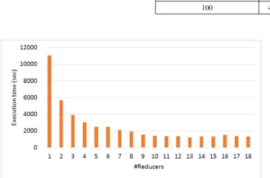
Fig. 10. Execution time with different numbers of reducers on Breast Cancer dataset withminsup=6.
C. Scalability
This section addresses the scalability of PaMPa-HD with respect to the number of reducers, since the most heavy operations (i.e., the execution of the “local” Carpenter) are executed by the reducers. The number of reducers varies from 1 to 18, which is the maximum number of tasks that can be run simultaneously in the commodity cluster at our disposal. The Breast cancer dataset and a minimum absolute support threshold equal to 6 have been used. As shown in figure V-C, the increase of the number of reducers has a positive impact on the execution time when the number of reducers is less than 10. The marginal benefits decrease as more reducers are added to the computation. Therefore, with more than 10 reducers, the benefits of the load distribution are compensated by the decreased effectiveness of the local pruning (i.e., the more the load is distributed, the less effective the local pruning is).
VI. RELATED WORK
Frequent itemset mining represents a very popular data mining technique used for exploratory analysis. Its popularity is witnessed by the high number of approaches and implementations. The most popular techniques to extract frequent itemsets from a transactional datasets are Apriori and Fp-growth. Apriori [11] is a bottom up approach: itemsets are extended one item at a time and their frequency is tested against the dataset. FP-growth [12], instead, is based on an FP-tree transposition of the transactional dataset and a recursive divide-and-conquer approach. These techniques explore the search space enumerating the items. For this reason, they work very well for datasets with a small (average) number of items per row, but their running time increases exponentially with higher (average) row lengths [11], [13].
14
In recent years, the explosion of the so called Big Data phenomenon has pushed the implementation of these techniques in distributed environments such as Apache Hadoop [1], based on the MapReduce paradigm [14], and Apache Spark [2]. Parallel FP-growth [9] is the most popular distributed closed frequent itemset mining algorithm. The main idea is to process more sub-FP-trees in parallel. A dataset conversion is required to make all the FP-trees independent. BigFIM and DistEclat [15] are two recent methods to extract frequent itemsets. DistEclat represents a distributed implementation of the Eclat algorithm [13] an approach based on equivalence classes (groups of itemsets sharing the same prefixes), smartly merged to obtain all the candidates. BigFIM is a hybrid approach exploiting both Apriori and Eclat paradigms. Carpenter [3], which inspired this work, has been specifically designed to extract frequent itemsets from high-dimensional datasets, i.e., characterized by a very large number of attributes (in the order of tens of thousands or more). The basic idea is to investigate the row set space instead of the itemset space. A detailed introduction to the algorithm is presented in section III.
VII. APPLICATIONS
Since PaMPa-HD is able to process extremely high-dimensional datasets we believe it is suitable for many application (scientific) domains. The first example is bioinformatics: researchers in this environment often cope with data structures defined by a large number of attributes, which matches gene expressions, and a relatively small number of transactions, which typically represent medical patients or tissue samples. Furthermore, smart cities and computer vision environments are two important application domains which can benefit from our distributed algorithm, thanks to their heterogeneous nature. Another field of application is the networking domain. Some examples of interesting high-dimensional dataset are URL reputation, advertisements, social networks and search engines. One of the most interesting applications, which we plan to investigate in the future, is related to internet traffic measurements. Currently, the market offers an interesting variety of internet packet sniffers like [16], [17]. Datasets, in which the transactions represent flows and the item are flows attributes, are already a very promising application domain for data mining techniques [18], [19], [20].
VIII. CONCLUSION
This work introduced PaMPa-HD, a novel frequent closed itemset mining algorithm able to efficiently parallelize the itemset extraction from extremely high-dimensional datasets. Experimental results shos its scalability and its performance in coping with datasets characterized by up to 10 millions different items and, above all, an average number of items per transaction up to 5 millions, on a small commodity cluster of 5 nodes. PaMPa-HD outperforms state-of-the-art algorithms, by showing a better scalability than both Carpenter and PFP, and being more efficient than PFP in the distributed itemset extraction. We plan to apply this approach in the network data analysis domain and to develop an Apache Spark implementation. We also plan to improve the expansion threshold selection: an auto-tuning mechanism based on the specific data distribution might further unleash the algorithm potential.
ACKNOWLEDGEMENT
The research leading to these results has received funding from the European Union under the FP7 Grant Agreement n. 619633 (Project “ONTIC”).
REFERENCES
[1] D. Borthakur, “The hadoop distributed file system: Architecture and design,”Hadoop Project, vol. 11, p. 21, 2007.
[2] M. Zaharia, M. Chowdhury, T. Das, A. Dave, J. Ma, M. McCauley, M. J. Franklin, S. Shenker, and I. Stoica, “Resilient distributed datasets: A fault-tolerant abstraction for in-memory cluster computing,” inNSDI’12, 2012, pp. 2–2.
[3] F. Pan, G. Cong, A. K. H. Tung, J. Yang, and M. J. Zaki, “Carpenter: Finding closed patterns in long biological datasets,” inProceedings
of the Ninth ACM SIGKDD International Conference on Knowledge Discovery and Data Mining, ser. KDD ’03. New York, NY, USA:
ACM, 2003, pp. 637–642. [Online]. Available: http://doi.acm.org/10.1145/956750.956832
[4] M. Cuturi, “UCI machine learning repository. PEMS-SF data set,” 2011. [Online]. Available: https://archive.ics.uci.edu/ml/datasets/PEMS-SF
[5] J. Leskovec and A. Krevl, “SNAP Datasets: Stanford large network dataset collection,” http://snap.stanford.edu/data, Jun. 2014. [6] Pang-Ning T. and Steinbach M. and Kumar V.,Introduction to Data Mining. Addison-Wesley, 2006.
[7] M. L. data set repository, “Breast cancer dataset (kent ridge.” [Online]. Available: http://mldata.org/repository/data/viewslug/breast-cancer-kent-ridge-2 Last access: July, 15th 2015
[8] C. Borgelt, X. Yang, R. Nogales-Cadenas, P. Carmona-Saez, and A. Pascual-Montano, “Finding closed frequent item sets by intersecting transactions,” in Proceedings of the 14th International Conference on Extending Database Technology, ser. EDBT/ICDT ’11. New York, NY, USA: ACM, 2011, pp. 367–376. [Online]. Available: http://doi.acm.org/10.1145/1951365.1951410
[9] H. Li, Y. Wang, D. Zhang, M. Zhang, and E. Y. Chang, “PFP: parallel fp-growth for query recommendation,” inRecSys’08, 2008, pp. 107–114.
[10] “The Apache Mahout machine learning library. Available: http://mahout.apache.org/,” 2013.
[11] R. Agrawal and R. Srikant, “Fast algorithms for mining association rules in large databases,” inVLDB ’94, 1994, pp. 487–499. [12] J. Han, J. Pei, and Y. Yin, “Mining frequent patterns without candidate generation,” inSIGMOD ’00, 2000, pp. 1–12.
[13] M. J. Zaki, S. Parthasarathy, M. Ogihara, and W. Li, “New algorithms for fast discovery of association rules,” inKDD’97. AAAI Press, 1997, pp. 283–286.
[14] J. Dean and S. Ghemawat, “Mapreduce: simplified data processing on large clusters,” inOSDI’04, 2004, pp. 10–10.
[15] S. Moens, E. Aksehirli, and B. Goethals, “Frequent itemset mining for big data,” inSML: BigData 2013 Workshop on Scalable Machine
Learning. IEEE, 2013.
[16] A. Finamore, M. Mellia, M. Meo, M. Munaf`o, and D. Rossi, “Experiences of internet traffic monitoring with tstat,”IEEE Network, vol. 25, no. 3, pp. 8–14, 2011.
[17] Cisco, “Netflow.” [Online]. Available: http://www.cisco.com/c/en/us/products/ios-nx-os-software/ios-netflow/index.html Last access: July, 15th 2015
[18] D. Apiletti, E. Baralis, T. Cerquitelli, S. Chiusano, and L. Grimaudo, “Searum: A cloud-based service for association rule mining,” in Proceedings of the 2013 12th IEEE International Conference on Trust, Security and Privacy in Computing and
Communications, ser. TRUSTCOM ’13. Washington, DC, USA: IEEE Computer Society, 2013, pp. 1283–1290. [Online]. Available:
http://dx.doi.org/10.1109/TrustCom.2013.153
[19] D. Brauckhoff, X. Dimitropoulos, A. Wagner, and K. Salamatian, “Anomaly extraction in backbone networks using association rules,”
Networking, IEEE/ACM Transactions on, vol. 20, no. 6, pp. 1788–1799, Dec 2012.
[20] D. Apiletti, E. Baralis, T. Cerquitelli, and V. D’Elia, “Characterizing network traffic by means of the netmine framework,”Comput.