Deep Learning for genomic data analysis

(1)

F

ACULDADE DE

E

NGENHARIA DA

U

NIVERSIDADE DO

P

ORTO

Deep Learning for genomic data

analysis

Vítor Filipe Oliveira Teixeira

Mestrado Integrado em Engenharia Informática e Computação Supervisor: Rui Camacho (FEUP)

Second Supervisor: Pedro Ferreira (I3S)

(2)

(3)

Deep Learning for genomic data analysis

Vítor Filipe Oliveira Teixeira

Mestrado Integrado em Engenharia Informática e Computação

Approved in oral examination by the committee:

Chair: Doctor Name of the President

External Examiner: Doctor Name of the Examiner Supervisor: Doctor Name of the Supervisor

(4)

(5)

Abstract

Since the Human Genome Project that the availability of genomic data has been increasing. With the huge investments in research, genome sequencing technologies and techniques have been im-proving at a fast rate, resulting in a cheaper yet faster genome sequencing. Such amount of data enables an advanced and more detailed analysis, which leads to advances in research. Data gener-ated by sequencing methods, like RNA-Seq, can be used to generate gene expression data which contain key information about the molecular basis of dangerous diseases such as cancer. However, the publicly available gene expression data related to cancer has some issues related to its nature, namely the low number of available samples to study, as well as a huge class imbalance problem. Moreover, this data is highly complex as it has a high dimensionality due to the number of genes, and, because of that, a considerable computational power and efficient algorithms are mandatory in order to extract useful information and perform it in reasonable time, which can represent a constraint on the extraction and comprehension of such information.

In this work, we focus on the biological aspects of RNA-Seq and in the analysis of the created representations by deep learning methods, given the recent and increasing number of records bro-ken by this approach. We divided our study into two main branches. First, we built and compared the performance of several feature extraction methods as well as data sampling methods using classifiers that were able distinguish the RNA-seq samples of thyroid cancer patients from sam-ples of healthy persons. Secondly, we have investigated the possibility of building comprehensible descriptions of gene expression data by using Denoising Autoencoders and Stacked Denoising Au-toencoders as feature extraction methods. After extracting information related to the description built by the network, namely the connection weights, we devised post-processing techniques to extract comprehensible and biologically meaningful descriptions out of the constructed models.

(6)

(7)

Resumo

Desde o Human Genome Project que os dados genómicos se têm tornado de mais fácil acesso. Com os inúmeros investimentos na área, as tecnologias de sequenciação de genomas tornam-se mais avançadas e sofisticadas, permitindo assim uma sequenciação mais barata e mais rápida. Tal quantidade de dados permite uma melhor e mais avançada pesquisa, o que leva a novas descober-tas na área. Através dos dados de sequenciação, como RNA-Seq, podem ser obtidos dados de ex-pressão genética, que contêm informações importantes para perceber a base molecular de doenças perigosas, como por exemplo cancro. No entanto, os dados disponiveis publicamente possuem problemas no que diz respeito ao número de exemplos para a análise, e também uma grande dis-paridade no que diz respeito ao número de exemplos de diferentes tipos num determinado conjunto de dados. Para além disso, estes dados possuem uma elevada dimensionalidade devido ao número de genes, e, por isso, são necessários algoritmos eficientes e um grande poder computacional de maneira a analisar e extrair informação útil num tempo aceitável, o que representa uma barreira no que diz respeito à extração e interpretação da informação.

Neste trabalho focamo-nos principalmente nos aspectos biológicos do RNA-Seq e na análise das representações criadas usando métodos de deep learning, dado o número de recordes que estes métodos têm batido recentemente. O trabalho foi dividido em duas vertentes principais. Na primeira construímos e comparamos a performance de vários métodos de extração defeaturese métodos desamplingde dados usando classificadores que foram capazes de distinguir amostras de RNA-Seq de pacientes com cancro da tiróide de amostras de pessoas saudáveis. Em segundo lugar, foi investigada a possibilidade de construir boas descrições dos dados de expressão genética usando Denoising Autoencoderse Stacked Denoising Autoencoderspara extracção de features. Após o treino dos modelos foi realizado um pós-processamento dos pesos extraídos dos modelos de maneira a conseguir retirar informação importante acerca da função e relação entre os genes.

(8)

(9)

Acknowledgements

First of all, I would like to express my sincere gratitude to my supervisor, Rui Camacho, for his promptness and guidance, that always pointed me to the right direction whenever I needed the most, and for all the help and freedom he gave throughout this thesis.

I would like to thank Pedro Ferreira, my second supervisor, for all the valuable advices he gave me, for helping me with all the questions I had concerning molecular biology and for helping me validate the results. Without his passionate participation this thesis would not have the same value.

I also would like leave a special thanks to my friend Joel Mendes, for being such a good friend and as well as to all my friends at FEUP, for being with me throughout all these years and making it one of the best periods of my life.

To my parents, Joaquim Teixeira, Maria Oliveira and to my sister, Liliana Teixeira, my deepest heartfelt thank you, for always providing me with unfailing support and encouragement. I owe them what I am today and will be in the future.

Last but not least, a truly heartfelt thank you to my girlfriend, Bárbara Pires. For always being there when I needed the most, for standing by me through the best and the worst times and for always putting a smile on my face and giving me the strength to face all the problems.

(10)

(11)

”The greatest obstacle to discovery is not ignorance - it is the illusion of knowledge. Never tell people how to do things. Tell them what to do and they will surprise you with their ingenuity.”

(12)

(13)

2 Biological and technological concepts 5 2.1 Molecular Biology . . . 5 2.2 Biological Pathways . . . 8 2.3 Sequencing RNA . . . 9 2.4 Transcriptome assembly . . . 9 2.5 RNA-Seq Analysis . . . 10 2.6 File Formats . . . 14 2.7 Data repositories . . . 15 2.8 Data mining . . . 16 2.9 Deep learning . . . 22

2.10 Distributed computing technology and tools . . . 34

2.11 Conclusions . . . 35 3 Methodology 37 3.1 Problem overview . . . 37 3.2 Challenges . . . 38 3.3 Research methodology . . . 39 3.4 Chapter conclusion . . . 40

4 Implementation and Results 41 4.1 Implementation . . . 41

4.2 Results . . . 53

4.3 Chapter conclusions . . . 62

5 Conclusions and future work 63 5.1 Objective Fulfillment . . . 63

5.2 Future work . . . 63

References 65 A DL4J model configurations 73 A.1 Configuration file (POM) . . . 73

A.2 Available options for network configuration . . . 76

(14)

CONTENTS

A.4 Denoising Autoencoder . . . 78

(15)

List of Figures

2.1 DNA and RNA structures . . . 6

2.2 Protein coding gene structure . . . 7

2.3 DNA Splicing . . . 7

2.4 Genetic code table . . . 8

2.5 Typical RNA-Seq Analysis workflow . . . 10

2.6 iRap pipeline [FPMB14] . . . 13

2.7 Data-mining process (Adapted from [Kan12]) . . . 17

2.8 Example of confusion matrix for binary classification . . . 20

2.9 Bayes theorem . . . 21

2.10 Simple Feedfoward Neural Network . . . 23

2.11 (Top) Classical Momentum (Bottom) Nesterov Accelerated Gradient [SMDH13] 26 2.12 Architecture of a Restricted Boltzmann Machine . . . 30

2.13 Architecture of a simple Convolutional Neural Network . . . 31

2.14 Example features learned in a face detection CNN . . . 31

2.15 An unrolled Recurrent Neural Network . . . 32

2.16 Basic architecture of an Autoencoder . . . 33

4.1 Data pre-processing pipeline . . . 43

4.2 Example of 5-fold cross-validation on a dataset with 30 samples . . . 46

4.3 Example of a single Denoising Autoencoder . . . 48

4.4 Example of Stacked Denoising Autoencoder architecture used in the experiments 49

(16)

(17)

List of Tables

2.1 Available RNA-Seq tools . . . 14

4.1 Specifications of the machines used to perform the experiments . . . 42

4.2 Versions of the used tools in the platform . . . 46

4.3 Hyperparameters used to run the experiment . . . 53

4.4 Resulting performance of the different sampling methods (%) . . . 54

4.5 Hyperparameters used to run the SDAE experiment . . . 55

4.6 Resulting performance of the different feature extraction methods (%) and their average running time . . . 55

4.7 Functional analysis clustering using connection weights approach on the denoising autoencoder results having 303 DAVID IDs with a p-value threshold of 0.05 . . . 56

4.8 Functional analysis clustering using connection weights approach on the stacked denoising autoencoder results having 419 DAVID IDs (0.015% of the total number of genes) with a p-value threshold of 0.05 . . . 56

4.9 Functional analysis clustering using algorithm1on denoising autoencoder results having 407 DAVID IDs (0.00075% of the genes with high weights in each node) with a p-value threshold of 0.05 . . . 58

4.10 Functional analysis clustering using algorithm1on stacked denoising autoencoder results having 378 DAVID IDs (0.0015% of the genes with high weights in each node) with a p-value threshold of 0.05 . . . 60

(18)

(19)

List of Algorithms

1 Algorithm used to extract high weight genes . . . 51

2 Algorithm used to extract similarities between the extracted features and known human pathways . . . 53

(20)

(21)

Abbreviations

AdaGrad Adaptative Gradient

ADAM Adaptative Moment estimation

ADASYN Adaptative Synthetic

API Application Programming Interface

BAM Binary Alignment Map

CNN Convolution Neural Network

CPU Central Processing Unit

DAE Denoising Autoencoder

DL4J Deep Learning For Java

DNA Deoxyribonucleic acid

ENCODE Encyclopedia of DNA Elements

GEO Gene Expression Omnibus

GFF General Feature Format

GO Gene Onthology

GPU Graphical Processing Unit

GTF General Feature Format

GUI Graphical User Interface

HTML HyperText Markup Language

JVM Java Virtual Machine

KEGG Kyoto Encyclopedia of Genes and Genomes KPCA Kernel Principal Component Analysis MRDM Multi-Relational Data Mining

mRNA Messenger RNA

MSE Mean Squared Error

NCBI National Center for Biotechnology Information

ND4J N-Dimensional Arrays For Java

NGS Next-Generation Sequencing

NHGRI National Human Genome Research Institute

PCA Principal Component Analysis

POM Project Object Model

RAM Random Access Memory

RBM Restricted Boltzman Machine

RDM Relational Data Mining

ReLU Rectified Linear Unit

REST Representational State Transfer

RNA Ribonucleic acid

RNA-Seq RNA Sequencing

RNN Recurrent neural Networks

(22)

ABBREVIATIONS

SDAE Stacked Denoising Autoencoder

SMOTE Synthetic Minority Over-sampling Technique

SQL Structured Query Language

Tanh Hyperbolic Tangent

TCGA The Cancer Genome Atlas

tRNA Transfer RNA

TSV Tab Separated Values

VCF Variant Call Format

(23)

Chapter 1

Introduction

In this chapter the context of this work is briefly explained as well as the underlying motivations and issue that arrive when dealing with the problem described. Then we explain what we aim to obtain with this research and end with a brief explanation of the structure of this report.

1.1 Context

Cancer is a group of diseases that involve an uncontrolled growth and spread of abnormal cells and is known to be responsible for the death of millions every year1. While there is still no cure for these diseases, there is still the possibility of enhancing the quality of medical diagnosis and disease prognosis. There is, however, an inherent difficult that is specific to the cancer type. For instance, in thyroid cancer, the tumors are expressed as thyroid nodes, and, among them, 95% are benign, which raises the difficulty of the diagnosis [Uti05].

A biomarker is any substance, structure or process that can be measured in the body or its products and influence or predict the incidence of outcome or disease [O+93]. Biomarkers play a critical role in understanding molecular and cellular mechanisms that drive tumor initiation, main-tenance and progression. Early disease detection by biomarkers offers an effective opportunity for enhancing disease detection, improving patient prognosis and optimizing the use of drug therapy to each case and assessing clinical outcomes of treatment. Hence biomarkers are known to be useful in several phases of the disease [Pfa13]:

• Before diagnosis, they provide the potential for screening and risk assessment.

• As part of the diagnostic process, biomarkers can determine staging, grading, and selection of initial therapy.

• In the treatment phase, they can be used to monitor therapy success, select additional thera-pies or monitor recurrent diseases.

(24)

Introduction

That said, it is important that we continue the pursuit of such biomarkers in order to decrease the number of fatalities caused by the disease. Last decade’s advances in sequencing techniques had an huge impact on genomics and enabled an inexpensive production of large amounts of sequencing data [Mar08]. As such, RNA biomarkers have been the choice in cancer research [PSM15][BM13][Kis15] and can be discovered by analysing RNA-Seq data. RNA-Seq uses next-generation sequencing to reveal the presence and quantify the amount of RNA present in a cell at a given moment and can be used to determine differences in gene expression over different groups [WL09]. However, the analysis and interpretation of gene-expression data still presents to be a significant challenge due to the nature of the data. There are three main challenges that are often faced when trying to extract any meaning from gene-expression cancer data: the low sample size of the dataset, the high dimensional noisy data, and how to extract the information from it. As such, a careful data processing and efficient algorithms are a must in order to extract meaningful information from it.

1.2 Motivation and objectives

Next-generation sequencing techniques led to the sequencing of cancer and normal genomes within a matter of weeks at a low price. Given the high mortality associated with cancer, the research for prevention and cure should be of high priority. However, it is still a challenge for researchers to analyse the data and extract useful information from it given the high complexity and sparsity of the data.

Deep learning is getting more and more attention after being known to outperform commonly used methods for classification [HSK+12]. Although these methods are not fully understood they are known to perform well in various situations if tuned well, which is proven to be a rather difficult task [Ben12]. That said, it is important to study and assess their performance in important fields like genomics that can revolutionize nowadays molecular biology knowledge and lead to potential discoveries that can help on clinical diagnosis and disease prognosis.

Of the more than 50000 genes that a gene-expression dataset can contain, only a few are relevant to the problem. Extracting the ones that are relevant and studying their influence on the disease is the main goal of this thesis. Methods like Denoising Autoencoders, that aim to reduce the dimensionality of the data by being forced to compress the data into a lower feature space by minimizing the difference between the input data and the reconstruction of an intentionally corrupted input data, have been used to extract the most important features from gene-expression data, making it easier to analyse a lower subset of genes [TUCG15]. In this work we will use papillary thyroid carcinoma gene expression data from The Cancer Genome Atlas. We will study the best ways to deal with the inherent problems related to the nature of the data and will assess the performance of Stacked Denoising Autoencoders for feature extraction of gene-expression data. Stacked Denoising Autoencoders are composed of many Denoising Autoencoders and are able to extract more non-linearities within the data.

(25)

Introduction

In sum, in this work we will start by dealing with the challenges mentioned above, namely, the low number of samples, data noise and high dimensionality, and how to extract important information from such generated features. First, we will deal with the low number of samples by comparing the performance of different data sampling methods given different conditions. Then, we deal with the high number of features by using and comparing different feature reduction methods, including Denoising and Stacked Denoising Autoencoders, that are the main focus in this thesis. Finally, after having the number of features reduced to a sensible number, we want to be able to extract comprehensible biological meaning from them in order to be able to help biologists discover novel cancer biomarkers. We will use several ways to extract the genes that most contributed for the generated features by analysing the final weights from the trained models. After having a list of what we call high weight genes we will try to cluster the genes using a functional annotation clustering tool in order to detect patterns and relations between the extracted genes and conclude if the generated features from the autoencoders have any biological meaning.

1.3 Structure of the thesis

Apart from this introductory chapter, the report has four additional chapters. Chapter2contains a detailed explanation on the state-of-the-art in topics relevant for the thesis work. We start by introducing the biological and genomic concepts needed to understand the given problem as well as RNA-Seq analysis and the most commonly used tools to generate and analyse gene-expression data. Furthermore, we also explain the concepts behind data mining and deep learning methods that we will use to analyse the data and present some of the most commonly used tools. The chapter ends with the description of relevant distributed frameworks that can be used in order to accelerate generation and analysis of gene-expression data.

In Chapter3we give a more deep overview of the problem and the challenges that arise when trying to solve it. We finish by explaining what was our rational behind our devised solution. Chapter4 describes and explains all of the implementation details, from the choice of the used tools and the pre-processing of the data to the way we implemented each step necessary to perform a given experiment. Chapter 5 concludes the thesis work and explain the difficulties that were found found during development stage. Future work is also part of Chapter 5.

(26)

(27)

Chapter 2

Biological and technological concepts

In this chapter begin by making an introductory approach to RNA-Seq and its underlying knowl-edge. Then, we will briefly review data mining algorithms and lastly introduce deep learning main concepts and the most commonly used deep learning and distributed frameworks.

2.1 Molecular Biology

DNA

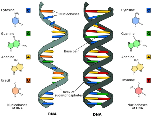
DNA is known to be the key molecule in every living organism as it carries the genetic information concerning each individual. It can be found at a cell’s nucleus1wrapped in a thread-like structure called chromosome in eukaryotic organisms or in the cytoplasm for prokaryotes.

DNA stands for Deoxyribonucleic Acid. DNA molecules are formed by two strands that form a double-helix. Those strands are composed of nucleotides. Each nucleotide contains a sugar (deoxyribose), a phosphate group and one nitrogenous base. There are four bases that can be present on DNA: Cytosine, Adenine, Guanine and Thymine. These bases are held onto each other by hydrogen bonds, connecting nucleotides thus forming the double stranded shape. There are, however, some base pairing rules. Each base cannot be paired with any other. Adenine can only be paired with Thymine and Guanine with Cythosin. [DNA] (Figure 1)

RNA

RNA stands for Ribonucleic Acid and is a molecule responsible for the coding, decoding, regu-lation and expression of genes [Cla08]. RNA and DNA have a similar structure, however, RNA only has a single strand that folds onto itself and its sugar is Ribose. It is composed of four types of ribonucleotide bases: Adenine, Cytosine, Guanine and Uracil. (Figure2.1)

1_{and also in mitocondria but not wrapped in chromosomes}

2_Image _taken _from: _{http://www.differencebetween.net/science/}

(28)

Biological and technological concepts

Figure 2.1: DNA and RNA structures2

Gene expression – from DNA to RNA to Proteins

DNA determines the structure of a cell, meaning whether it is meant to be an eye cell, a skin cell and so forth [RS08]. DNA contains genes and those genes are used to produce RNA (the transcription process) that has the information needed to synthesize a protein in a process called gene expression [CH16].

A gene is a continuous string of nucleotides that begins with a promoter and ends with a ter-minator. They can also contain regulatory sequences that can increase or decrease the expression of the specific gene. (Figure 2).

The process of transforming DNA into proteins is divided in two stages: transcription, where RNA is produced using DNA templates and translation, where proteins are synthesized using RNA templates.

Transcription occurs inside the nucleus and itself can be divided in three stages: initiation, elongation and termination. In the initiation stage, the RNA polymerase binds to the promoter re-gion of the gene where the majority of the gene expression is controlled. As the RNA polymerase binds to the DNA, it separates the two strands. Then, in elongation the RNA polymerase slides along the DNA while adding complementary nucleotides to the new forming RNA. Finally, in

(29)

ter-Biological and technological concepts

Figure 2.2: Protein coding gene structure3

mination, the RNA polymerase reaches the terminator, pre-mRNA is completed and it disconnects from both RNA polymerase and DNA.

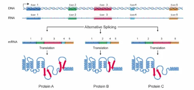
The mRNA that is formed during transcription contains coding and non-coding sections, exons and introns, respectively. Since only exons contain information on how to synthesize a protein, introns are then removed by spliceosomes in a process called splicing [CH16]. (Figure2.3)

Figure 2.3: DNA Splicing4

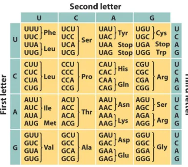
After this stage, the pre-mRNA (precursor messenger RNA) is now matured and contains only coding information that is ready to be translated. This new formed mRNA contains groups of three nucleotides called codons. Each codon translates into a specific amino acid according to the

3_{Image taken from: http://web2.mendelu.cz/af_291_projekty2/vseo/print.php?page=307&typ=html} 4_{Image taken from: https://en.wikipedia.org/wiki/Alternative_splicing}

(30)

genetic code table, except for four codons: AUG, the start codon, and UAA, UAG, UGA, the stop codons [CH16]. (Figure2.4)

The translation process is also divided into three stages: Initiation, elongation and termination. The initiation stage begins with the small subunit ribosome scanning the mRNA to find the start codon. Then, the initiator tRNA, which contains the amino acid corresponding to the codon, connects to the start codon and the large ribosomal subunit connects to form the initiation complex. After the initiation is complete, the elongation starts. In this stage, tRNA (transfer RNA) connects to the subsequent codons, one at a time, and a chain of amino acids is formed as the ribosome moves along the strand. When the ribosome reaches a stop codon, the polypeptide is released and the complex is dissociated so that the process can start again at initiation.

Figure 2.4: Genetic code table5

2.2 Biological Pathways

A biological pathway is a sequence of interactions between molecules in a cell that result in a cer-tain product of changes in a cell [Bio]. Those interactions aim to control the flow of information, energy and biochemical compounds in the cell and the ability of the cell to change its behavior in response to a stimuli.

There are several types of biological pathways with the most commonly known ones being metabolic, signaling and gene-regulation pathways. These are very important to understand the mechanisms that originate a disease as they provide clues on what genes, proteins and other molecules are involved in the pathway. Comparing two pathways, from a healthy person and from a person with a disease, researchers can find what triggered such disease.

(31)

2.3 Sequencing RNA

Sequencing can be defined as figuring out the order of the nucleotides in an orgamism’s DNA. Sequencing methods have been continuously improving throughout the years [HC16]. From tak-ing years and billions of US$ to sequence a human genome ustak-ing Sanger’s methods like in the Human Genome Project, which took thirteen years to be completed and US$ 3 billion [Hay14], to being able to sequence a human genome in a day for less than US$ 5000 using next-generation sequencing [SLS+10].

Next-generation sequencing (NGS), otherwise known as deep or massively parallel sequencing refers to the technological advances in sequence techniques that enable a huge number of sequence reads6 per run [Met09]. By allowing an high throughput and decreased cost compared to other sequencing technologies [Hay09], this method gained popularity among researchers.

Such advances gave birth to a new technique called RNA-Seq (RNA Sequencing) [WL09]. RNA is of huge importance when it comes to gene expression, combining that with NGS tech-niques enables the profiling of whole transcriptomes while offering a cost-effective way of mea-suring genome-wide expression..There are plenty of next-generation sequencing platforms, each one with its own use However, the most commonly used is the Illumina/Solexa7.

These advances also enabled new projects like [AA+15] to be completed, resulting in more data available for analysis. Nevertheless, it is still a challenge to analyse the huge datasets we get from the above mentioned technology as seen further ahead in this thesis.

2.4 Transcriptome assembly

A transcriptome is the collection of all RNA present in a cell or tissue and the corresponding quantity. RNA sequences are "mirrors" of the DNA from which they were transcribed, considering Thymine is replaced by Uracil, and such, by analysing all RNA sequences in a cell (transcriptome), we can estimate which genes are more expressed in a cell or tissue [WGS09]. That information is of major importance, for instance, if a gene is highly expressed in a cancer cell that can mean that it could be associated with the growth of the cell, giving the researchers some insight on gene functions that were not previously known like in [TJWJ11].

RNA sequences are obtained experimentally using sequencing methods and are assembled in partial or complete transcriptomes.

For many years, microarrays were the standard tool for genomic-wide transcriptome analysis. This approach, however, has some downsides compared to the recent RNA-Seq methods. This is mainly because RNA-Seq works with both reference-based assembly andde novo assemblies [WGS09]. In reference-based methods the aligning of the short reads is made with a reference genome or transcriptome while inde novomethod we can obtain a transcriptome without the aid of a reference genome. This approach gained a particular interest among researchers because

6_{A read is a fragment of a a genome/transcriptome obtained by sequencing methods} 7_{Illumina: http://www.illumina.com/}

(32)

it widened the possibilities of DNA analysis [CLS+11] and the creation of new transcriptomes for organisms that have an incomplete reference genome or don’t have one yet at all. Hence, researchers developed various ways of improving this approach [EB+11].

2.5 RNA-Seq Analysis

A single run from any sequencing platform generates a quite big amount of data. For instance, the average human genome size can go up to 200GB of data [GEN] which represents a challenge when it comes to computational resources. That said, powerful computational resources and good algorithms are a must when performing the analysis.

RNA-Seq can be used for various research, such as findings in alternative splicing [PSL+08], gene-expression quantification and transcripts [CLS+11,MWM+08], detecting gene fusions [EMK+11,

PTS+10] and some more variations.

RNA-Seq Analysis workflow

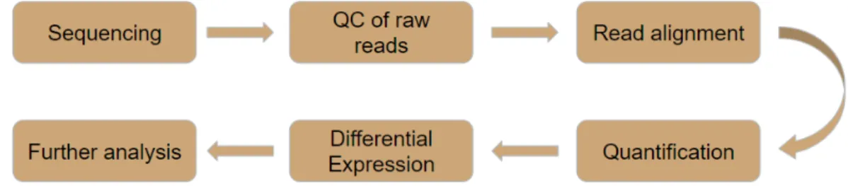
The RNA-Seq analysis workflow consists, broadly, of the steps shown in (Figure 5).

Figure 2.5: Typical RNA-Seq Analysis workflow

Before explaining the concepts of each step, one should have in mind that these steps are not always followed. Nodes can be added and/or removed depending on the goal of the analysis.

After obtaining the raw reads in the sequencing process the reads are subjected to a quality control step. In this step tools are used in order to "clean" the data and improve further stages performance. These tools are used to discard low-quality reads, trim adaptor sequences8 and eliminate poor-quality bases [CMT+16].

After the quality control step, the reads will be aligned with ade novoassembly, if the reference genome is not present, or with the reference genome or transcriptome otherwise.

Following the alignment step a quantification is performed. In this step reads are aggregated in order to calculate gene expression values to be then compared with other samples values in the differential expression step in order to know what genes are most expressed.

8_{Single or double-stranded chemically synthesized short fragments of nucleic acids that can be ligated to the ends}

(33)

Gene analysis

After having identified which genes are differentially expressed, performing an analysis is the core step to extract any meaning from the result. Gene Ontology (GO) project provides a set of structured, controlled vocabularies for the community use in annotating genes and gene product attributes across all species [GO07]. These, so called GO terms, have a name, a unique alphanu-meric identifier, a definition with cited sources, and a namespace with the domain where it belongs. Gene Ontology is structured as a direct acyclic graph where each term is connected to one or more terms in the same, or other domain. These terms cover three domains:

Cellular component, the parts of a cell or its extracellular environment.

Molecular function, the elemental activities of a gene product at the molecular level, such as binding or catalysis.

Biological process, operations or sets of molecular events with a defined beginning and end, pertinent to the functioning of integrated living units: cells, tissues, organs, and organisms.

The assignment of a GO term to a gene product is called annotation which are useful to un-derstand the relationships between genes on a gene set. This process is called gene enrichment analysis and can be performed using various tools that provide enrichment capabilities, for in-stance, PANTHER9, DAVID10or gProfiler11.

Tools for RNA-Seq

In this subsection we will present some of the most relevant tools for the RNA-Seq steps described previously.

FastQC

FastQC12 is a quality control tool used to clean data coming from next-generation sequencing methods. It accepts any FastQ, SAM and BAM files, which are file formats that will be described with more depth below in this thesis, and provides an overview of the problematic areas in a form of graph or table as well as the option to export the results as an HTML (HyperText Markup Language) report.

T-Coffee

T-Coffee is a multiple sequence alignment tool that can be used to align sequences or join multiple sequences from different alignment methods [NHH00]. It uses a progressive approach that consists in aligning the two most closely related sequences and then successively align the next most related

9_{http://pantherdb.org/} 10_{https://david.ncifcrf.gov/} 11_{http://biit.cs.ut.ee/gprofiler/}

(34)

ones. Although it does not guarantee an optimal solution, this approach is efficient enough to implement on large scale datasets.

BLAST

BLAST, which stands for Basic Local Alignment Search Tool [AGM+90], and is a widely used tool for sequence searching. It finds regions of similarity between sequences by comparing those sequences to sequence databases and calculates a statistical significance between them.

Bowtie

Bowtie is a short read alignment tool. It is meant to be a memory-efficient option that works best when aligning large sets of short reads to large genomes. Bowtie indexes the reference genome using a method called Burrows-Wheeler transform to perform the alignment to make the alignment memory efficient, that can take advantage of multiple processors in order to speed up the alignment process.

Bowtie 2 [LS12] is a new improved version of Bowtie that achieves an higher speed, sensivity and accuracy by using dynamic programming algorithms and a full-text minute index.

TopHat

Tophat [TPS09] is a mapping tool for RNA-Seq reads. It uses Bowtie as a short read aligner and then analyses the mapping results to identify splice junctions between exons. While other alignment tools rely on known splice sites, TopHat enables the discovery of new ones by mapping to a reference genome after the alignment.

Cufflinks

Cufflinks [TRG+12] is a transcript assembler that estimates their abundance and tests for differen-tial expression and regulation in RNA-Seq samples. Its package contains several different internal tools such as: Cufflinks, that is used to assemble the transcripts, Cuffcompare, used to compare the assembly to known transcripts, Cuffmerge, used to merge the transcript assemblies, Cuffquant, used to quantify gene and transcript expression in RNA-Seq, having the option to save the results as a file that can be latter analysed with Cuffdiff, used to compare expression levels of genes and transcripts and Cuffnorm used to normalize them.

DESeq

DESeq [AH10] is an R package used to analyse count data from RNA-Seq and test differential gene expression. It uses a negative binomial distribution to infer differential signal correctly and with good statistical power as count data is discrete and skewed therefore is not well approximated by a normal distribution.

(35)

EdgeR

EdgeR [RMS09] is an R package included in the Bioconductor software packages. It used to perform differential analysis of RNA-Seq expression profiles and implements a wide range of statistical methods based on negative binomial distributions.

iRAP - Integrated RNA-seq Analysis Pipeline

Each step in the RNA-Seq Analysis workflow can be performed with multiple tools, each one having its pros and cons. Integrating them can also be a problem since the input/output of each tool may not be compatible, which can make it hard for someone who does not have the necessary skills to apply these techniques.

In order to solve that problem the iRap pipeline will be desribed. iRap is a pipeline for RNA-Seq that integrates various tools needed for filtering and mapping reads, quantifying expression and testing for differential expression [FPMB14].

Figure 2.6: iRap pipeline [FPMB14]

As seen in Figure. 6, iRap uses two more steps to complement the analysis of RNA-Seq, gene set enrichment and web reports. The gene set enrichment step is useful in order to understand gene expression data. This method focus on gene sets instead of focusing in single genes [STM+05] which adds more meaning to the results. Web reports make it easier to understand and observe the results produced in each stage of the analysis [FPMB14].

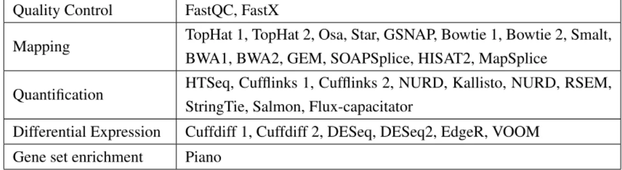
Tools supported by iRap

(36)

Quality Control FastQC, FastX

Mapping TopHat 1, TopHat 2, Osa, Star, GSNAP, Bowtie 1, Bowtie 2, Smalt,

BWA1, BWA2, GEM, SOAPSplice, HISAT2, MapSplice

Quantification HTSeq, Cufflinks 1, Cufflinks 2, NURD, Kallisto, NURD, RSEM, StringTie, Salmon, Flux-capacitator

Differential Expression Cuffdiff 1, Cuffdiff 2, DESeq, DESeq2, EdgeR, VOOM Gene set enrichment Piano

Table 2.1: Available RNA-Seq tools

2.6 File Formats

FASTA

A FASTA format [FAS] file contains text file information concerning nucleotides or peptide se-quences. It consists of a description line followed by the correspondent sequence representation. The description line begins with a ">" followed by the name and/or the sequence identifier. This format is extremely simple making the file parsing and conversion easy to do.

FASTQ

The FastQ format is quite similar to FASTA, it also contains text file information about nucleotides. However, it has an extra complementary sequence with the associated per base quality scores [CFG+09].

Each sequence is usually represented in four lines. The first line starts with an "@" followed by its ID. The next line corresponds to the raw sequence letters followed by the third line, containing a "+" with an optional ID. The last line contains the quality scores for the sequence in line two.

This format can be seen as an extension of the FASTA format since it also provides the ability to store quality scores as well as avoiding the big title lines without any line wrapping that would often make common parsers crash [CFG+09]. This format has become the standard for storing the output of high-throughput sequencing instruments like Illumina.

SAM and BAM

SAM stands for Sequence Alignment/Map. This format is tab-delimited and it is used to store sequence data aligned to a reference sequence [LHW+09]. The file consists in a header section and alignment section, and, since it is stored in plain-text it is easy to read and parse. The only thing that differs from BAM to SAM files is their encoding. Instead of using plain text, BAM files store the same information in binary format, thus increasing performance by allowing compression and fast random access [LHW+09].

(37)

VCF

Variant Call Format (VCF) is a text file format used to store information about variants found at certain positions in a reference genome [DAA+11]. It was first developed for the 1000 Genomes Project in order to deal with the problem of storing all the information about the genome.

A VCF file contains the header, which includes the file format version and the variant caller version, and the data lines which include the information about the variant.

BED

The BED (Browser Extensible Data) format is used to represent genomic features and annotations [USC]. BED files are tab-delimited and each line contains three mandatory fields, the chromosome name, its starting and ending position, and nine optional fields containing more information about each feature.

GFF and GTF

The Generic Feature Format (GFF) is a text file format used to store gene features. These files are tab-delimited and consist of one line per feature, each one containing nine fields and an optional track line [USC].

Gene Transfer Format (GTF) files are similar to GFF, that is, GTF files are a refinement of the GFF format. The first eight fields are the same but the last one is now expanded into a list of attributes that provide more information about each feature.

2.7 Data repositories

In order to test and validate the results we should use real data to assess the performance of our so-lution. For that we can use public databases containing genome information such as TCGA13(The Cancer Genome Atlas), which contains data from hundreds of cancer samples using NGS tech-niques. This genomic information helps researchers to increase the knowledge about cancer pre-vention, diagnosis and treatment. There is also another huge source of information called The ENCODE Project14 which is funded by the NHGRI (National Human Genome Research Insti-tute) and its goal it contains a list of the functional elements in the human genome. In addition to these last repositories we also have GEO15(Gene Expression Omnibus) that is a public repos-itory for high throughput data at NCBI. It has available tools to help users query and download experiments and curated gene expression profiles.

13_{https://cancergenome.nih.gov/} 14_{https://www.encodeproject.org/} 15_{https://www.ncbi.nlm.nih.gov/geo/}

(38)

2.8 Data mining

Data mining can be seen as the process of extracting knowledge and discovering important pat-terns from data [HPK11]. Data is getting more and more abundant and it seems ever-increasing. Nowadays, due to the ease of acquiring more storage and more computational power we store ev-ery little bit of information we would otherwise throw away some years ago. Consequently, as the abundance of data grows and the machines that can perform these type of tasks become common-place, also does the need of understanding what that data means, as important information can be extracted from it. That same information is what attracted people and companies into using data mining, the search of something new and nontrivial in large amounts of data.

Most existing data mining approaches look for patterns in single data tables, called proposi-tional data mining. While they are useful for not very complex datasets, for datasets which have multi table relations that approach will result in loss of meaning or information. RDM (Relational Data Mining), often referred to as MRDM (Multi Relational Data Mining) is an approach that aims to solve that problem. RDM looks for patterns that involve multiple table relations [Dže03] in order to deal with the complex real world data. These approaches have been applied to a variety of areas, remarkably in the area of bioinformatics like in [FCC11].

Two of the main goals in data mining are considered to be prediction and description [FPSS96,

Kan12]. Prediction is when the learning algorithm uses the current data to make future predictions whilst description tries to characterize the properties of the data in a given dataset [HPK11].

There are plenty of ways to achieve these goals and extract useful information from data which will be briefly explained below.

Classificationalgorithm tries to classify data into finite number of predefined labels (class val-ues) by learning a function that maps objects to the labels.

Regression tries to build a predicting learning function that maps an element to the real-value predicted by the function.

Summarization is a descriptive task that tries to represent data in a more concise way while maintaining the main features of the dataset.

Clusteringis a descriptive task that tries to identify a set of clusters or categories to define similar data. There is a clustering subfield called conceptual clustering that aims to not only cluster the data but also discover and explain the meaning behind each cluster.

Anomaly detection tries to find unusual values, that is, values that deviate from what is nor-mal in the dataset. These values are considered outliers and can be either considered errors or interesting values that should be further investigated.

(39)

Model-evaluationtries to find dependencies between variables or values of a feature in a dataset.

General approach on problem solving

There is a general procedure to data mining problem solving that involve the five following steps (Figure 2.7):

We first start by stating the problem and formulating an hypothesis followed by collecting the needed data to perform the mining. Before performing it the data should be cleaned in a step called pre-processing. For the extraction to be efficient we should gather only the needed information in order to get better and faster results. After we remove outliers or select the features that we want in pre-processing we can implement and use the appropriate data-mining technique. After the data mining the results need to be validated in order to then draw conclusions on them. We need to be sure that the results that we got from the analysis are relevant and not wrong, otherwise they will be useless and misused.

Figure 2.7: Data-mining process (Adapted from [Kan12])

Pre-processing

One of the steps in the problem solving pipeline that is of huge importance is data pre-processing. Missing this step would cause the results of the analysis to be misleading.

TCGA gene expression data is of huge dimensionality, given the number of analysed genes, and imbalanced, as it often has a much bigger number of cancer samples compared to the samples from healthy patients.

(40)

That leads us to two known problems in data science, dimensionality reduction, and imbal-anced datasets.

Dimensionality reduction

Dimensionality reduction is the process of discovering compact representations of high-dimensional data [RS00]. Genomic data is of very high dimensions so a feature extraction method can be useful to extract and analyse its compact representation in comparison with the raw data. The methods that appear to be useful for the problem are the following:

PCA (Principal component analysis) is a linear technique whose goal is to encode high-dimensional data into a lower high-dimensional representation. It finds the most important information within the data and generates a set of orthogonal variables called principal components that best differentiate the data points [AW10]. In sum, the principle behind this method is the maximization of the variance of the orthogonal transformation of the raw data.

KPCA, orKernel PCA, is an extension of PCA, however, unlike PCA, KPCA tries to find a low-dimensional nonlinear space [SSM98]. It uses kernel methods to compute the principal com-ponents in high-dimensional feature spaces.

Autoencodersare a type of artificial neural network that is commonly used for unsupervised learning. Autoencoders try to encode the data and reconstruct it while minimizing the error, finding compact representations of the data. They will be covered in more depth in2.9.

Imbalanced datasets

More and more we deal with an issue that is often present in nowadays data, namely imbalanced datasets, the lack of samples of one class. When presented with an imbalanced dataset classifiers will often be biased towards the majority class, failing at learn the difference between the majority and minority class. While there is no silver bullet that can solve this challenge entirely, there are some techniques that can be used to help [HG09].

Algorithm modificationis a procedure that is more oriented to the adaptation of the base learning methods to be more sensitive to imbalanced classes.

Cost-sensitive learningcan be useful when the data is well-known as samples of the minority class can be given more importance compared to sample classes that appear more often.

Data samplingis a way of modifying the dataset by some mechanisms in order to balance it. Resampling can be done in several ways, either by undersampling, oversampling or hybrid methods that combine both strategies [LFG+13].

(41)

The basic methods involve random oversampling and undersampling where samples are du-plicated and removed, respectively. However, these strategies were proven not to be the best since they have no heuristic, as such, downsides arrive with the mentioned problem, random over-sampling often leads to overfitting, while random underover-sampling can lead to the elimination of important samples [HG09].

That said, better approaches have been developed. One such example is SMOTE, synthetic mi-nority oversampling technique [CBHK02]. With this technique, the minority class is oversampled based on the feature space similarities between its samples. To create a synthetic sample, it con-siders the K-nearest neighbors and randomly selects one to multiply its feature vector difference by a random number between 0 and 1 and adds this vector to the selected neighbor. This approach, however, has some drawbacks as when it is generating synthetic samples it doesn’t consider neigh-boring examples, which can lead to over generalization and increases the overlapping between classes [HG09][LFG+13]. In order to deal with this drawback, adaptive sampling methods such as Adaptive Synthetic Sampling (ADASYN) have been proposed. ADASYN uses a method to create data according to their distributions, that is, more samples are generated for minority class samples that are harder to learn compared to samples that are easier to learn [HBGL08]. In addi-tion to ADASYN, there are also other ways to deal with the issues of SMOTE with one of them being using it with data cleaning techniques like SMOTE + Tomek or SMOTE + ENN [BPM04] that clean the unwanted overlapping between classes after the oversampling, each one using dif-ferent methods for the task.

Performance measures

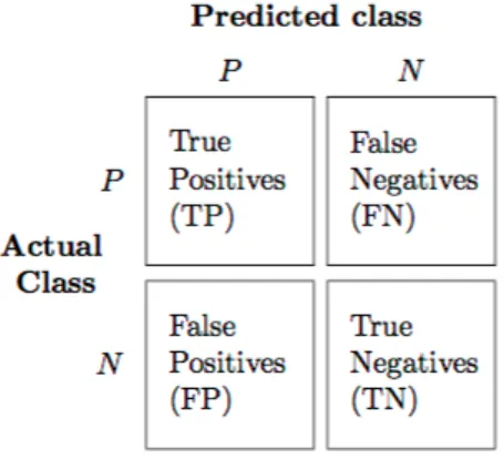
Evaluating the performance of a model is one of the core steps in a data mining process. It indicates how successful predictions of a dataset have been by a trained model. The performance of a classification can be evaluated by four different values: the number of correct predictions of class examples (true positives, correctly identified), the number of correct predictions that don’t belong to the class (true negatives, correctly rejected), the number of examples that were incorrectly assigned to a class (false positives, incorrectly identified) and the number of examples that were not recognized as being of the class (false negatives, incorrectly rejected)[SL09]. These four values form a matrix, often called confusion matrix that is shown in2.8as an example for binary classification.

(42)

Figure 2.8: Example of confusion matrix for binary classification16

There are some metrics that are used that are based on the values of the confusion matrix that are listed below:

Accuracy

Accuracy is the overall effectiveness of a classifier.

Accuracy= T P+T N

T P+T N+FP+FN

Precision

Precision is the proportion of the classes that were correctly identified by the classifier.

Precision= T P

T P+FP

Recall

Recall is the effectiveness of a classifier to identify positive labels.

Recall= T P

T P+FN

F1 Score

F1 Score is the harmonic mean of both precision and recall. It is an important metric to use when assessing the performance of classifiers in unbalanced datasets.

F₁= 2T P 2T P+FP+FN

16_Image _taken _from _{http://rasbt.github.io/mlxtend/user_guide/evaluate/confusion_}

(43)

Classification techniques

In this subsection we will briefly explain some of the commonly used classification algorithms. Logistic Regression

Logistic Regression is a statistical method used for analysing a dataset in which there are one or more independent variables that output a binary outcome. Its goal is to find the best fitting model as a linear combination of the predictor variables.

Support Vector Machines

Support Vector Machines are used as a classifier algorithm where a separating hyperplane is de-fined in order to separate the classes. The hyperplane is optimal when it has the largest distance to the nearest point in both training classes.

Artificial Neural Networks

Artificial Neural Networks are commonly used for classification using a special activation function on the last layer called softmax. In order to perform classification using artificial neural networks the last layer needs to have as many neurons as the number of classes and the activation of the layer will be the probability of the input being of a given class. Softmax function will be discussed further ahead in this thesis.

Decision trees

Decision trees are a method used for classification. The goal is to create a model that can predict the value of a variable given several input variables. In decision trees, each non-leaf node repre-sents input features and each leaf node on the tree reprerepre-sents the resulting value for that variable given the path from the root to the node. There are many algorithms for building decision trees such as ID3 or C4.5.

Naive Bayes

Naive Bayes are a commonly used classification algorithm based on Bayes Theorem. It lies on the principle that every feature that is being classified is independent of the value of any other feature, being that the reason behind being called naive. They are pretty simple to implement and one of the main reasons to use them is the speed. By being given a set of features being probabilities it can predict what is the class that has the highest probability for the given input.

P(A|B) =P(B|A)P(A)

P(B)

(44)

Data Mining tools

In this subsection we will list some of the most used tools for data mining purposes.

WEKA

WEKA17stands for Waikato Environment for Knowledge Analysis. It is an open source tool that contains a collection of machine learning used for data mining tasks. It is written in Java and it is extensible, meaning that we can easily implement new functionalities given the need. It can be used through a command line or directly by its GUI.

RapidMiner

RapidMiner18 is a complete solution for data mining and machine learning problems. It is used for business and commercial purposes as well as for educational and research ones. It supports all steps of the data mining process detailed in figure2.7 and its functionalities can be extended through the use of new plugins. This software platform is priced by the amount of data used by the models and its only free up to 10000 rows of data for non-educational purposes while for educational purposes its free to use.

R

R19is a statistical computing language for data analysis and graphics. This language can be con-sidered a different implementation of the S language. It contains several statistical and graphical techniques and can be easily extended. It is commonly used among statisticians and data miners given its wide variety of functionalities.

KNIME

KNIME20is an open source data analytics that integrates various components for machine learning and data mining. It is popular for its modular pipelining concept. KNIME allows processing of large data volumes and integrates with various open-source projects like Weka and the R project that we mentioned before.

2.9 Deep learning

Deep Learning is a subfield of machine learning, so, before being able to understand deep learning it is mandatory to know what is machine learning and how are computers able to learn. Machine learning is a computer science field that tries to give a machine the ability to learn. Learning is the

17_{http://www.cs.waikato.ac.nz/ml/weka/} 18_{https://rapidminer.com/}

19_{https://www.r-project.org/} 20_{https://www.knime.org/}

(45)

process of learning something either by experimentation/studying or getting taught. There are two types of learning, supervised and unsupervised.

Supervised and unsupervised learning Supervised Learning

Supervised is the type of learning where we help the computer determine what it needs to achieve by giving it the desired results along with the input in the training data. The goal of this type of learning is to generalize, that is, it needs to know how to get the correct results for inputs that were not present in the training set. A common problem of this kind of approach is overfitting. Overfitting is when the model learns the data instead of learning the function, so when presented with new data that was not present in the training set it performs poorly because it is too adapted to the training set. It usually happens when the dataset is too small or homogeneous.

Unsupervised Learning

Unsupervised learning is when the desired output is not given during the training. It is used to find the structure or the relationship between the given data, like, for instance, clustering, which is one of the most commonly used unsupervised learning methods.

Deep Neural Networks

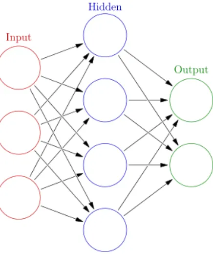
Deep learning is a buzzword that derives from artificial neural networks. An artificial neural network is an information processing paradigm that was inspired by the way a biological brain works. Artificial neurons are connected to many others by links that act like axons, thus connecting the output of one neuron to the input of another one (Figure2.10). These links have numeric weights that represent the strength of the connection between two nodes. Those weights can be tuned based on experience, making neural networks capable of learning based on the input.

(46)

There is no general concensus on the definition of deep neural network but it can be seen as any artificial neural network that has several hidden layers, more than two most of the times. By having multiple layers these networks are able to learn representations of the data with multiple levels of abstraction [GBC16]. Over the last years this approach has been gaining a lot of interest due to the fact that it outperforms the common used methods for classifying on various datasets [HSK+12] and improved the state-of-art in various fields like speech and image recognition [LBH15] and also in drug discovery and genomics [DGH16].

Training the models - Backpropagation

Backpropagation is the common method to use when training an artificial neural network. It is commonly used with an optimization method called gradient descent. Gradient descent is an op-timization algorithm that is used to find a local minimum of a function, called the cost or error functions. There are three variations of gradient descent [Rud16]:

Batch gradient descent

This approach is the standard gradient descent. It computes the computes the gradient of the cost function with respect to the parametersθas follows:

θ=θ−η·∇θL(θ)

Where we calculate the gradients of the full training set before performing one update, which can be rather slow for big datasets or even very difficult to do when datasets don’t fit in memory.

Stochastic gradient descent

With stochastic gradient descent, instead of passing through the whole training set for a single update, it performs a parameter update for each training sample like follows:

θ=θ−η·∇θL(θ;x

(i)_,_y(i)₎

Wherex(i),y(i)are a given sample of the training set.

This approach solves the problem where the dataset is too big to fit in memory and, in addition to this, has a faster convergence, since it avoids the computation of similar values on each param-eter update. Nevertheless, it can lead to some fluctuations on the minimization of the objective function.

Mini-batch gradient descent

The mid-term between the above two approaches is mini-batch gradient descent. Instead of updating for every training set sample the updates are performed in mini-batches, a small set of training samples:

(47)

θ =θ−η·∇θL(θ;x(

i:i+n)_,_y(i:i+n)₎

Wherex(i:i+n),y(i:i+n)are elements from a batch with size n.

By choosing a small batch of data, this approach reduces the fluctuations of the parameter updates in comparison to the updates from a stochastic approach.

A forward pass and a backward pass of all training examples is called epoch. In other words, an epoch is completed after the network as seen all dataset samples. On the other hand, an iteration is completed after each mini-batch is processed. The number of iterations on each epoch depends on the size of the mini-batch.

In the case of neural networks gradient descent is used to find the optimal value for each weight, since its optimal value is at the global minimum, which sometimes can’t be satisfied because gradient descent can get stuck in a local minimum, being one of its limitations. Choosing a learning rate, that is, how quickly the weights are updated, can be rather difficult. A high learning rate can make the loss function diverge, and a small learning rate will lead to a slow convergence. Learning rate schedules [DCM] try to solve this problem by adjusting the learning rate according to some schedule, however, since they have to be defined beforehand, they cannot adapt to the characteristics of the data set. In addition to this, we might want to vary the learning rate according to the frequency of samples of a given dataset, that is, if we have few samples that map to a characteristic we might want to have a larger update in that case. Algorithms with adaptive learning rates deal with the challenges aforesaid and will be briefly described below.

In sum, backpropagation tries to find the minimum of the error function in the weight space using gradient descent. The general steps of the algorithm in a neural network are as follows:

1. Initialize network weights and biases

2. Weights are propagated forward through the network 3. The output error is calculated

4. Compute hidden and input layers weights by calculating the partial derivative of the error function with respect to the given weight

5. Update network weights by multiplying the negative of the computed partial derivatives with the learning rate

6. Repeat until stop condition is met

Gradient Descent Optimization Algorithms

As we mentioned earlier, there are some challenges with respect to the learning rate hyperpa-rameter. In order to deal with that, many improvements on the basic stochastic gradient descent algorithm have been proposed throughout the years. We will briefly explain two of the most com-monly used methods below.

(48)

Nesterov accelarated gradient

When in areas where the surface is steeper in one dimension more than in another, Stochastic Gradient Descent has some troubles and oscillates around that area making small progress, thus taking more time to converge. Momentum [Qia99] is a method that helps stopping the "zig-zag" when we go down to a local minimum. The current step now depends on both the current gradient and the change on the last step so that it accelerates the convergence and pushes it in the right direction while minimizing the oscillation.

υt+1=γ υt−η∇θL(θ)

θ=θ+υt+1

Whereυt is the current velocity vector andβ is the momentum parameter.

However, when reaching towards the minimum, momentum is often high and it doesn’t slow down causing it to miss the minimum entirely and going further to a not so good solution. In order to solve that issue, Nesterov accelerated gradient [Nes83] was created.

υt+1=γ υt−η∇θL(θ+γ υt)

θ=θ+υt+1

Instead of using gradient at the current location and then taking a big step in the direction of momentum, it first takes a big step in the direction of the accumulated gradient and then makes a correction based on the gradient.

Figure 2.11: (Top) Classical Momentum (Bottom) Nesterov Accelerated Gradient [SMDH13]

AdaGrad

AdaGrad [DHS11] is an adaptive gradient algorithm that adapts the learning rate to the parameters. This is very useful for sparse data where features that are highly informative are not very abundant in the training data. When they appear in the training process they are going to be weighted equally comparing to a feature that is present in a lot of training samples and is not very informative.

(49)

AdaGrad tries to solve that imbalance by increasing the learning rate for more sparse parameters and decreasing for less sparse ones.

gt =∇θL(θ) θt+1=θt− η √ Gt+ε gt.

WhereGt is a diagonal matrix that contains the sum of the squares of the past gradients with respect to all theθparameters andεa small value, usually 10(−8), to avoid division by zero.

ADAM

ADAM [KB14], or Adaptive Moment Estimation is an adaptive gradient algorithm that can be seen as a generalization of AdaGrad. The update rule for Adam is based on the estimation of first (gradient mean) and second (uncentered variance) order moments of past gradients.

mt =β1mt−1+ (1−β1)gt vt =β1vt−1+ (1−β2)g2t ˆ mt= mt 1−β₁t ˆ vt = vt 1−β₂t

Wheremt andvt are estimations of first and second order moments, respectively and ˆmtand ˆvt are the correction bias.

Then, the correction bias are used to update the parameters like follows:

θt+1=θt− η √ ˆ vt+ε ˆ mt Cost functions

Cost functions can also be viewed as the loss, or error of a model. In a simplistic way, they are the difference between what the model think is the correct result and the actual correct result. The objective of backpropagation is to minimize this function in order to infer the right weights. Here we will list some of the most common cost functions.

Mean Squared Error

MSE=1 n n

∑

i=1 (yi−yˆi)2

(50)

Where n is the total number of items in the training data, y is the true value and ˆy is the estimated value.

The mean squared error function measures the average of the squares of the errors, that is, the difference between the output value we got and what we estimated.

Cross-Entropy

C=−1

n

∑

_x [ylnα+ (1−y)ln(1−α)]

Where n is the total number of items in the training data,α is the output from the neuron, the sum over all training inputs, x, and y is the desired output.

This function is often used when the data is normalized as its results are bounded between 0 and 1 and can be represented as probabilities.

Kullback-Leibler Divergence DKL(P||Q) = n

∑

i=1 P(i)lnP(i) Q(i)

WhereDKL(P||Q) is a measure of the information lost when Q is used to approximate P, in other words, it measures the "distance" between two distributions. Unlike other Euclidean distances, KL-Divergence is not symmetric, that is, whenQ(i) =0 andP(i)!= 0.

Activation functions

For any hidden layer to provide any useful information we need to use a non-linear activation function, otherwise it doesn’t matter how deep the network is, the results will always yield a linear transformation, which won’t produce any useful information given the non-linearity in real-world problems. Here we list some of the commonly used activation functions in this field.

Sigmoid

f(x) = 1 1+e−x

The sigmoid function was known to be the most used activation function. One of the reasons for it is that the derivatives needed for the gradient descent are easy to calculate. Other reason is that they are bounded between 0 and 1 and it can be used as a probability estimation.

There are however some downsides of using this function like the vanishing gradient problem where the gradient gets exponentially smaller in the early layer leading to a slow training process. To solve this problem researchers are using ReLU activation function that we will see below. An-other factor to take into account is that it contains exponentials which is an expensive operation and slows down the process.

(51)

f(x) = 2 1+e−2x−1

Tanh function, commonly known as hyperbolic tangent, is another type of activation function that is quite similar to the sigmoid. However, this function’s derivatives are higher than sigmoid’s so it has stronger gradients [LBOM98b]. It also has a greater range [-1,1] than the sigmoid’s [0,1], avoiding bias in the gradients. As well as the sigmoid function, it also has the downside of having to calculate exponentials.

ReLU

f(x) =max(0,x)

ReLU, also known as Rectified Linear Unit is an activation function that has no bounds. It trans-lates any negative input to 0 and all positive values are kept. This function is now the most popular non-linear activation function in use [LBH15]. Two of the main reasons is that it is fast, and it avoids the vanishing gradient problem that the sigmoid and tanh functions have. It has, however, another problem which is usually called the "dying ReLU". This occurs when some neuron always outputs the same value, that is, it gets stuck at 0 because the function gradient at 0 is also 0. One approach to deal with this problem is the the use of a "Leaky ReLU" or the "Exponential ReLU" [CUH15]. Instead of translating a value to 0 if it is negative we can modify the flat side of the function for it to have a gradient and give the neuron a chance to recover.

LeakyReLU: f(x) = ( x i f x>0 0.01x i f x≤0 ELU: f(x) = ( x i f x>0 α(ex−1) i f x≤0 Softmax Sj= ezi ∑NK=1eak ∀j∈1..N

The softmax function is mainly used as the activation function of an output layer using cross-entropy loss for multi-class classification. It takes an N dimensional vector of real values and produces another N dimensional vector of values in the range 0 to 1 that can be interpreted as the probability of a given input being of the given class.