Estimation of Gaussian Networks and Modular Brain Functional Networks

(1)

Estimation of Gaussian Networks and Modular Brain

Functional Networks

A THESIS

SUBMITTED TO THE FACULTY OF THE GRADUATE SCHOOL OF THE UNIVERSITY OF MINNESOTA

BY

Chen Gao

IN PARTIAL FULFILLMENT OF THE REQUIREMENTS FOR THE DEGREE OF

Doctor of Philosophy

Wei Pan, Ph.D.

(2)

c

Chen Gao 2017

(3)

Acknowledgements

I am grateful to my advisor, Professor Wei Pan, for his guidance and encouragement.

(4)

Abstract

Graphical models are intuitive tools to demonstrate dependence relation between vari-ables of interest. Both undirected and directed graphical models are widely used in many applications, such as reconstructing gene expression/co-expression networks and brain functional networks. A popular model for undirected graphs is the Gaussian graphical model, where conditional independence can be inferred from the absence of an edge in the graph. Another approach for estimating undirected graphs does not depend on the distribution of the data. Instead, the resulting network is constructed through transfor-mation of empirical sample correlation and node connectivity. The estimated network connectivity measures can be used as a secondary phenotype for association tests with genotypes. Finally, new methods have been proposed to estimate directed Gaussian graphs. The direction of an edge allows easier interpretation of causal relation between nodes in the graph.

We first aim to estimate multiple Gaussian graphs in the presence of sample hetero-geneity, where the independent samples may come from different and unknown popula-tions or distribupopula-tions. We embed in the framework of a Gaussian mixture model one of two recently proposed methods for estimating multiple precision matrices in Gaussian graphical models. Secondly, we adapt a weighted gene co-expression network analysis (WGCNA) framework to resting-state fMRI (rs-fMRI) data to identify modular struc-tures in brain functional networks. We propose applying a new adaptive test built on the proportional odds model (POM) that can be applied to a high-dimensional setting, where the number of variables (p) can exceed the sample size (n) in addition to the usual p < n setting. Finally, we implemented a new method for estimating directed acyclic graph (DAG) as an R package, and demonstrated its use via application to a real data set and simulation studies.

(5)

List of Tables

2.1 Simulation results with n = 173 and the true model being that esti-mated byone of the three methods based on the glioblastoma dataset. The means (standard deviations) of the Rand Index (RI), adjusted Rand Index (aRI), average entropy loss (EL) average quadratic loss (QL), aver-age false positive for sparseness pursuit (FPV), averaver-age false negative for sparseness pursuit (FNV), average false positive for grouping (FPG) and average false negative for grouping (FNG) are shown for 50 simulations. 16 2.2 Simulation results with n = 346 and the true model being that

esti-mated byone of the three methods based on the glioblastoma dataset. The means (standard deviations) of the Rand Index (RI), adjusted Rand Index (aRI), average entropy loss (EL) average quadratic loss (QL), aver-age false positive for sparseness pursuit (FPV), averaver-age false negative for sparseness pursuit (FNV), average false positive for grouping (FPG) and average false negative for grouping (FNG) are shown for 50 simulations. 26 2.3 Rand Index (RI) and adjusted Rand Index (aRI) for the glioblastoma

gene expression data with 20 genes by various methods. The class as-signments given in [1] are used as the reference. . . 27 3.1 P-values of the tests for SNP-whole network associations using the

cor-relation, covariance, TOM or adjacency matrix elements as the net-work connectivity measure respectively. W-mod and Btw-mod stand for within-modular and between-modular, respectively. . . 39 3.2 P-values of the tests for SNP-individual network module associations

us-ing the correlation, covariance, TOM or adjacency matrix elements as the network connectivity measure. . . 40

(8)

4.2 % of non-zero elements for data set simulated from Model 2. . . 57 4.3 Mean of the estimated parameters for data set simulated from Model 1. 57 4.4 Mean of the estimated parameters for data set simulated from Model 2. 57 4.5 % of non-zero elements for data set simulated from Model 3. . . 58 4.6 % of non-zero elements for data set simulated from Model 4. . . 59 4.7 Mean of the estimated parameters for data set simulated from Model 3. 59 4.8 Mean of the estimated parameters for data set simulated from Model 4. 59 4.9 % of non-zero elements for the estimated graphs from Model 5. Sample

sizen= 100. D stands for the gDAG package, G stands for the graphical lasso, and T stands for the graphical lasso with TLP. Non-zero percentage of the true edges were highlighted for the gDAG package. . . 61 4.10 % of non-zero elements for the estimated graphs from Model 5. Sample

sizen= 1000. D stands for the gDAG package, G stands for the graphical lasso, and T stands for the graphical lasso with TLP. Non-zero percentage of the true edges were highlighted for the gDAG package. . . 62

(9)

List of Figures

2.1 Estimated cluster-specific networks based on 173 core samples using the new method New-SP. . . 19 2.2 Estimated cluster-specific networks based on 173 core samples using the

method of Zhou et al. (2009). . . 20 2.3 Estimated cluster-specific networks based on 173 core samples using the

method of New-JGL. . . 21 2.4 Distributions of the CV log-likelihood values of various fitted models

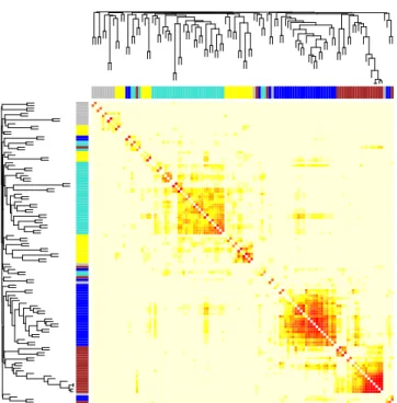
based on bootstrap samples. Null-Null, bootstrap samples were gener-ated from the null model, to which the null model was fitted; Null-Alt, bootstrap samples were generated from the null model, to which the al-ternative model was fitted; Alt-Null, bootstrap samples were generated from the alternative model, to which the null model was fitted; Alt-Alt, bootstrap samples were generated from the alternative model, to which the alternative model was fitted. The two horizontal lines are the CV log-likelihood values for the two fitted models to the original data. . . . 23 3.1 TOM plot of the whole brain functional network and its modules for

normal subjects. The rows and columns are the ROIs, ordered by their distance in the tree. . . 36 3.2 TOM plot (top), covariance matrix plot (middle) and correlation matrix

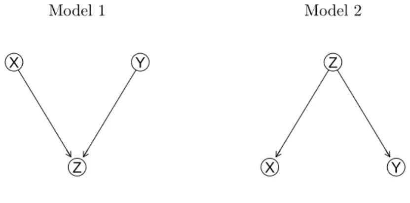
plot (bottom) of the brain functional networks for the three genotype groups based on APOE4 SNP (rs429358) (with its minor allele counts equal to 0, 1 or 2 from left to right). . . 38 4.1 Plot of the estimated DAG for the simulated data set. . . 56 4.2 True DAG for Model 1 and Model 2. . . 56

(10)

selected tuning parameter was indicated by the dashed horizontal line. . 58 4.4 Solution paths of the graphical lasso for Model 2. The median of the

selected tuning parameter was indicated by the dashed horizontal line. . 58 4.5 True DAG for Model 5. . . 60 4.6 The estimated graph using thegDAG(top) or the graphical lasso (bottom)

for the pooled samples, control cohort and the case cohort. The nodes for SNPs were relocated to corners for comparison. . . 60

(11)

Chapter 1

Introduction

Graphical models are widely used to illustrate dependence relation between variables. A typical graph G is composed of V the set of nodes andE the set of edges. An edge in E indicates dependence between two nodes that are connected by the edge. The nodes and edges in a graphical model also forms a network. In this work, network and graph are used interchangeably. The application of graphical models includes gene expression networks [2, 3], brain functional networks [4, 5], social networks [6] and so on. This thesis focuses on statistical methods related to estimation and statistical testing of graphs.

The Gaussian graphical model, which is based on multivariate normal distribu-tion (also called the Gaussian distribudistribu-tion), is an example of the graphical models. A non-zero off-diagonal element Σ−_ij1 in the inverse covariance matrix Σ−1 corresponds to independence of the two variables i, j, conditional on all other variable [7]. Estima-tion of a Gaussian graphical model is equivalent to estimaEstima-tion of the inverse covariance matrix in the Gaussian distribution. However, when the dimension of variables p ex-ceeds the number of samples n in the data set, the empirical covariance matrix of the Gaussian distribution cannot be inverted. Estimation of the Gaussian graphical model in high-dimensional setting has become an interesting topic. A variety of methods use penalty terms to constrain the parameter space of the inverse covariance matrix, and successfully transforms the task to a constrained optimization problem [8, 2]. While these methods for estimating Gaussian graphs are popular, there is a need to estimate multiple graphs with commonnalities as suggested by real-world evidence [1]. Recently,

(12)

new methods have proposed to address the problem of estimating multiple Gaussian graphs [9, 3]. These new methods can be adapted to estimate multiple networks in the presence of sample heterogeneity, where the independent samples (i.e. observations) may come from different and unknown populations or distributions. In low-dimensional setting, the parameters in a Gaussian mixture model can be obtained via the EM algo-rithm [10]. In high-dimensional setting, penalization is needed for parameter estimation [11, 12]. By recognizing the relation between Gaussian graphical models and Gaussian mixture models, we embed in the EM algorithm one of two recently proposed methods for estimating multiple precision matrices in Gaussian graphical models. We demon-strate the feasibility and potential usefulness of the proposed methods in an application to glioblastoma subtype discovery and differential gene network analysis with a microar-ray gene expression data set. Our method is able to achieve simultaneous discovery of unknown disease subtypes and detection of differential gene (dys)regulations in func-tional genomics. We also conduct realistic simulation studies to evaluate and compare the performance of various methods.

Graphical models can be applied to construct brain functional networks[13, 14]. Dis-ruption of connectivity in the brain functional network is related to many pathological conditions in the brain, such as Alzheimer’s disease, Schizophrenia [15, 16]or autism [17]. A brain functional network may consist of records of more than 100 regions of interst (ROIs) [18]. Due to its high dimensionality and high noise levels, analysis of a large brain functional network may not be powerful. While some investigators restricted their analysis a smaller network with fewer ROIs [18], another line of approaches aims to decompose a large network into smaller subcomponents called modules. Although several methods exist for estimating brain functional networks, such as the sample cor-relation matrix or graphical lasso for a sparse precision matrix [19], it is still difficult to extract modules from such network estimates. Motivated by these considerations, we adapt a weighted gene co-expression network analysis (WGCNA) framework [20] to resting-state fMRI (rs-fMRI) data to identify modular structures in brain functional networks. Modular structures are identified by using topological overlap matrix (TOM) elements in hierarchical clustering. We propose applying a new adaptive test built on the proportional odds model (POM) that can be applied to a high-dimensional setting [21], where the number of variables (p) can exceed the sample size (n) in addition to

(13)

the usualp < nsetting. We applied our proposed methods to the ADNI data to test for associations between a genetic variant of the APOE4 allele and either the whole brain functional network or its various subcomponents using various connectivity measures. We uncovered several modules based on the control cohort, and some of them were marginally associated with the APOE4 variant and several other SNPs.

The graphical models discussed in Chapter 2 and 3 estimate undirected graphs, and the edges in undirected graphs do not have directions. The direction of dependence cannot be inferred from the edges in the undirected graphs. In contrast, directed graphs consist of directed edges between nodes. The directed edges have intuitive interpretation of causal relation of the nodes in a graph. Of particular interest is the directed acyclic graphs (DAGs) models, which exclude directed circles in the graph. Several methods have been proposed for estimating DAGs. For the low-dimensional setting where the number of nodes is relatively small, a few methods have been proposed by either reducing the search space [22] or greedy search[23]. However, these methods struggles in the high-dimensional setting because the search space grows super exponentially in the number of nodes [24]. Another class of methods originated from the PC algorithm [25], which uses conditional independence relationship to delete recursive edges from an undirected graph. Kalisch and B¨uhlmann [25] adapted the PC algorithm for estimating the skeleton of DAGs in the high-dimensional setting. Recently, Yuan et al. developed a new approach for estimation of DAGs in highdimensional setting. In this article, we first introduced the method for estimation of directed acyclic Gaussian graph, and implemented this method as the R package gDAG. We also reviewed the graphical lasso and its extension as competing methods for estimating graphs. We compared the performance of gDAG with graphical lasso and other competing methods. We also demonstrated an application of the gDAG package to the gene expression and SNP data set by Webster et al. [26].

Chapter 2 describes a new method for estimating Gaussian graphs in Gaussian mix-ture model setting. Chapter 3 applies a weighted network model for the estimation of brain functional networks. Adaptive association test is applied to test for the associa-tion between network connectivity measures and genotypes. Chapter 4 describes an R package that implements a new method for estimating directed acyclic graphs.

(14)

Chapter 2

Estimation of multiple networks

in Gaussian mixture models

2.1 Introduction

We consider the problem of estimating multiple networks in the presence of sample heterogeneity; that is, the samples come from several populations with different Gaus-sian distributions, however it is unknown which samples are from which distributions. The precision matrix of each distribution corresponds to a network. This is related to but differs from the usual task of inferring and contrasting multiple networks in Gaus-sian graphical models, where it is known which samples are from which distributions (Guo et al. 2011; Danaher et al. 2014; Zhu et al. 2014 [27, 3, 9]). Although Gaus-sian mixture models are widely used for model-based clustering, our primary goal is for estimation and comparison of cluster-specific precision matrices, for which existing model-based clustering methods (McLachlan and Peel 2001; Fraley and Raftery 2006; Zhou et al. 2009 [28, 29, 12]) are not suitable. The existing model-based clustering methods either specify a common precision matrix or estimate multiple unconstrained cluster-specific precision matrices; due to the lack of a fusion penalty or other mech-anisms, the cluster-specific precision matrix estimates are either exactly the same or completely different. On the other hand, in many applications one would expect both commonalities and differences among the cluster-specific precision matrices. Account-ing for their commonalities not only improves statistical estimation efficiency through

(15)

information borrowing, but also enhances the ability of interpretation with a focus on few possible changes across the cluster-specific precision matrices.

Our proposed methods were motivated by genomic applications to disease subtype discovery while accounting for differential gene expression and/or differential gene reg-ulations across (unknown) disease subtypes. This is in contrast to existing methods allowing for only differential gene expression in disease subtype discovery (Verhaak et al. 2010 [1]). Arguably, a biologically more interesting problem is not only in detecting differential gene expression, but also in discovering gene dysregulations, across to-be-discovered disease subtypes, which will facilitate understanding disease mechanisms and thus developing individualized treatments.

Our approach is in the framework of multivariate Gaussian mixture modeling (McLach-lan and Peel 2001 [28]). The majority of the existing literature on mixture modeling focus on regularizing only the mean parameters with diagonal covariance matrices (Pan and Shen 2007; Wang and Zhu 2008; Xie et al. 2008 [11, 30, 31]), though some (Zhou et al. 2009; Hill and Mukerjee 2013; Wu et al. 2013 [12, 32, 33]) have started considering regularization of the covariance parameters too, all of which, however, do not touch on the key issue of identifying both common and varying substructures of the precision matrices across the components of a mixture model. Since these methods always give different networks for different populations unless a common network is assumed, they do not address the question of interest here: which parts of the networks change with the populations. To address this question, we propose embedding one of the current methods of estimating multiple Gaussian graphical models (Danaher et al. 2014; Zhu et al. 2014 [3, 9]) in the EM algorithm (Dempster et al. 1977 [10]) for the Gaussian mixture model, for which existing algorithms can be effectively used in the M-step of an EM algorithm for a Gaussian mixture model.

Since these methods apply a fusion penalty to shrink multiple networks towards each other, they not only are statistically more efficient with information borrowing, but also facilitate interpretation in identifying differential network substructures. In particular, due to the use of a non-convex penalty, the method of Zhu et al. (2014) [9] strives to uncover the commonalities among multiple networks while maintaining their unique substructures too.

(16)

Due to the connections to and differences from our current problem, we briefly re-view the literature on Gaussian graphical models without sample heterogeneity; that is, it is known that the samples come from the same Gaussian distribution. Gaussian graphical models are commonly used to describe conditional dependence relationships between interacting variables for continuous multivariate data. They are widely applied to reveal the structures in gene regulatory networks ([34, 35]), protein interaction net-works ([2, 36, 37]) and brain functional connectivity ([38, 37]). Each network or graph consists of a set of nodes representing variables (e.g. genes) and edges; each edge be-tween two nodes indicates the conditional dependency of the two nodes, given all other nodes. In Gaussian graphical models, the edges between nodes are determined by the non-zero off-diagonal elements in the precision matrix (the inverse of the covariance matrix). Therefore, reconstruction of the graph is equivalent to estimating the preci-sion matrix in the Gaussian graphical model. Friedman et al. (2008) [2] proposed the graphical lasso method to estimate the (inverse) covariance matrices, where they pro-vided an efficient algorithm to directly maximize theL1-penalized log-likelihood. While

the graphical lasso is fast, it only focuses on estimating a single graph. It ignores the structural similarities of multiple graphs when graphical lasso is applied to estimate each graph separately. Recent works aim to recognize possible commonalities among multiple graphs. Peterson et al. (2015) [39] proposed a Bayesian approach to estimate multiple Gaussian graphs by placing a Markov random field prior on the edges and a spike-and-slab prior to control the similarity between graphs. Qiu et al. (2015) [40] proposed a kernel method for joint estimation of multiple Gaussian graphs. Guo et al. [27] proposed to control the sparsity of the off-diagonal elements of the precision matrices and to use the L1 penalty to control the differences between the off-diagonal

elements for each pair of precision matrices. Danaher et al. (2014) [3] proposed the joint graphical lasso algorithm, which uses theL1 penalty to regularize both the sparsity and

the differences between the corresponding off-diagonal elements for each pair of preci-sion matrices. Mohan et al. (2014) [41] extended the joint graphical lasso by taking a node-based approach for estimation of multiple Gaussian graphs. Recently, Zhu et al. (2014) [9] proposed a regularized maximum likelihood method for estimation of multiple precision matrices, In addition to seeking sparseness with a non-convex penalty to reg-ularize the off-diagonal elements in each precision matrix, it also imposes a non-convex

(17)

fusion penalty on the differences between each pair of some related precision matrices that can be flexibly specified.

The rest of this paper is organized as follows. In Section 2 we introduce our proposed new methods for estimating component-wise precision matrices in the framework of a Gaussian mixture model. Section 3 presents simulation studies to demonstrate the promising performance of our proposed methods, followed in Section 4 for an application to a glioblastoma gene expression data set. We conclude in Section 5 with a summary of our findings.

2.2 Methods

2.2.1 Gaussian mixture model

We assume that each of n iid p-dimensional observations, x1, x2, . . . , xn, comes from a

Gaussian mixture distribution with probability density function

f(xj) = g

X

i=1

πifi(xj;θi),

where g is the number of components (or populations), πi is the prior probability for

componentiwithPg

i=1πi= 1,θi ={µi, Vi}is the set of the mean and covariance matrix

parameters for cluster i, and fi is a multivariate Normal density (with a

component-specific mean µi and covariance matrix Vi),

fi(x;θi) = 1 (2π)p/2_|_V i|1/2 exp −1 2(x−µi) 0_V−1 i (x−µi) .

Since each component corresponds to a cluster, we will refer to component and cluster exchangeably. The primary goal here is to estimate the cluster-specific precision matri-ces Wi =Vi−1, though identifying the clusters is often of interest either as a direct or

side product.

Given the data, the log-likelihood is

logL(Θ) = n X j=1 log g X i=1 πifi(xj;θi) ! , (2.1)

where Θ = {(πi, θi) : i = 1,2, ..., g} denotes the set of all unknown parameters. An

(18)

likelihood estimates. For high-dimensional data, it is often beneficial to use the maxi-mum penalized likelihood estimator based on a penalized log-likelihood

logLP(Θ) = logL(Θ)−pλ(Θ), (2.2)

wherepλ(Θ) is to be specified as a penalty on all or a subset of the parameters. Various

penalties have been proposed to achieve better performance in different contexts.

2.2.2 New methods

New method 1: with a convex penalty

A zero entryWi;kl, the (k, l)th entry ofWi, indicates conditional independence between

thekth andlth variables in clusterigiven other variables. Estimating multiple cluster-specific precision matrices can reveal changes of dependency structures across multiple clusters. To facilitate detecting structural changes, a penalty is imposed on the differ-ences between the corresponding entries across multiple precision matrices. We propose using a joint lasso and fused graphical lasso (FGL) penalty of Danaher et al. (2014) [3] on each precision matrices Wi’s:

pλ(Θ) =λ1 g X i=1 X k6=l |Wi;kl|+λ2 X i<i0 X k,l |Wi;kl−Wi0_;_kl|, (2.3)

where λ1 and λ2 are nonnegative tuning parameters. In addition to achieving

sparse-ness as in graphical lasso, FGL also encourages identical entries across cluster-specific precision matrices. This feature helps to reveal both commonalities and cluster-specific network structures, in addition to improving statistical estimation efficiency through borrowing information across the multiple networks.

Note that Danaher et al. (2014) used the above penalty in the context of Gaussian graphical modeling, knowing which observations are from which Gaussian distribution, differing from our Gaussian mixture modeling. Nevertheless, we will show how to apply their proposed ADMM algorithm ([42]) (as implemented in the R package JGL) in the M-step of an EM algorithm in the current context.

We denote the new method that incorporates the use of the joint lasso and fused graphical lasso (JGL) in our Gaussian mixture modeling as New-JGL.

(19)

New method 2: with a non-convex penalty

In the context of Gaussian graphical modeling, Zhu et al. (2014) [9] proposed the following non-convex penalty function for Wi,

pλ(Θ) =λ1 g X i=1 X k6=l Jτ(|Wi;kl|) +λ2 X i<i0 X k6=l Jτ(|Wi;kl−Wi0_;_kl|), (2.4)

where λ1, λ2 and τ are nonnegative tuning parameters, and Jτ(z) = min(|z|, τ) is the

truncated Lasso penalty (TLP) (Shen et al. 2012 [43]). The two penalties serve the corresponding sparseness and fusion roles as in JGL. However, in contrast to FGL in (2.3), only non-diagonal elements, but not diagonal elements, are penalized for their differences in (2.4).

The non-convex TLP reduces the bias induced by the lasso penalty because no more penalty is imposed if |z|> τ inJτ(z). In the current context, the TLP can do better

in maintaining the magnitudes of non-zero entries or differences between two unequal entries. The scaled TLP,Jτ(z)/τ, approximates theL0-function,I(z6= 0), asτ tends to

0+. Like FGL, this method is able to detect possible element-wise heterogeneity across multiple networks, for example in identifying signaling network changes across distinct cancer subtypes.

We propose using the same non-convex penalty (2.4) in our current context of Gaus-sian mixture modeling, and will demonstrate that the algorithm of Zhu et al. (2014) can be applied in the M-step of an EM algorithm for our purpose. We denote the new method that incorporates the use of structural pursuit (SP) penalty (2.4) in our Gaussian mixture modeling as New-SP(New-Structural-Pursuit).

2.2.3 Computing

We develop an EM algorithm to obtain the maximum penalized likelihood estimates (MPLEs). In particular, we will demonstrate how to use an existing Gaussian graphical modeling algorithm in the M-step of the EM algorithm for a penalized Gaussian mixture model.

We introducezij as the indicator of whether xj belongs to component i, sozij = 1

(20)

data. Ifzij’s are observed, the complete data penalized log-likelihood is logLc,P(Θ) = g X i=1 n X j=1 zij[logπi+ logfi(xj;θi)]−pλ(Θ), (2.5)

where pλ(Θ) is a penalty on the parameters; typically only the mean parameters µi’s

and/or covariance matrices Vi’s are penalized, which is assumed throughout.

Define the posterior probability ofxj’s belonging to component ias ρij = P(zij =

1|xj; Θ), then the E-step calculates the following with the current estimate Θ(r) at

iteration r, QP(Θ; Θ(r)) =EΘ(r)(logLc,P|X) = g X i=1 n X j=1 ρ(_ijr)[logπi+ logfi(xj;θi)]−pλ(Θ) (2.6) with ˆ ρ(_ijr) =P(zij = 1|xj; Θ(r)) = ˆ π(_ir)fi(x0j;θ (r) i ) Pg i=1πˆ (r) i fi(x 0 j;θ (r) i ) . (2.7)

In the M-step, we find ˆπ(_ir+1), ˆµ_i(r+1)and ˆW_i(r+1)that maximizeQP. Using the Lagrange

multiplier η to constrain Pg

i=1πi = 1, we omit the terms without πi’s and rewrite QP

as L(π, η) = g X i=1 n X j=1 ˆ ρ(_ijr)logπi+η( g X i=1 πi−1). (2.8)

Taking the partial derivative of L(π, η) with respect toπi and set it to 0, we arrive at

the updating formula for ˆπi

ˆ π(_ir+1) = n X j=1 ˆ ρ(_ijr)/n. (2.9)

To update µi, if there is no penalty onµi, we take the derivative ofQP with respect to

µi and set it to 0, ∂QP ∂µi = n X j ˆ ρ(_ijr)(xj−µi)0Wˆi= 0, (2.10)

obtaining the updating formula for ˆµi as

ˆ µ(_ir+1) = Pn j=1ρˆ (r) ij xj Pn j=1ρˆ (r) ij . (2.11)

(21)

On the other hand, if the Lasso penalty is imposed on µi, then its updating formula

involves a soft-thresholding on the above quantity (e.g., Pan and Shen 2007 [11]). Finally, to updateVi or equivalently, Wi =V_i−1, we only need to consider the terms

related to Wi inQP: QP = 1 2 g X i=1 n X j=1 ˆ ρ(_ijr)log|Wi| − 1 2 g X i=1 n X j=1 ˆ ρ(_ijr)(xj−µˆ(_ir))0Wi(xj−µˆ(_ir))−pλ(Θ) = 1 2 g X i=1 n X j=1 ˆ ρ(_ijr)log|Wi| −tr( ˜Si(r)Wi) −pλ(Θ) (2.12) with ˜ S_i(r)= Pn j=1ρˆ (r) ij (xj−µˆ(ir))(xj−µˆ(ir))0 Pn j=1ρˆ (r) ij (2.13)

as a weighted sample covariance matrix.

Typically there is no closed-form solution to update Wi or Vi when one of them

is penalized. However, we can take advantage of the existing methods for penalized Gaussian graphical models. Below we point out their connection.

If we know the cluster label for each observationxj, as in Gaussian graphical

mod-eling, then the penalized log-likelihood for Wi is

1 2 g X i=1 [ni(log|Wi| −tr(SiWi))−pλ(Wi)], (2.14)

where ni is the sample size for cluster i, and Si is the sample covariance matrix for

cluster i. Correspondingly, in the current context of Gaussian mixture modeling, the

QP function in the EM algorithm with a penalty on Wi is

QP = 1 2 g X i=1   n X j=1 ˆ ρ(_ijr) log|Wi| −tr( ˜Si(r)Wi) −pλ(Wi)  . (2.15)

To maximize QP, we use the soft assignment, instead of hard assignment, of each

observation xj into a cluster. Specifically, setting ni =Pn_j₌₁ρˆ_ij(r) and Si = ˜S_i(r), then

maximizing expression (2.15) will be equivalent to maximizing (2.14). Since there are al-ready efficient computational algorithms to maximize the penalized log-likelihood (2.14) in the Gaussian graphical model, we can incorporate one of them into the M-step in our EM algorithm to obtain an update for Wi. Zhou et al. (2009) used this idea in

(22)

applying graphical Lasso (Friedman et al. 2008 [2]) in their penalized model-based clus-tering with unconstrained covariance matrices. We applied the R functions of Danaher et al. (2014) and Zhu et al. (2014) in the M-step for the proposed two new methods respectively.

2.2.4 Review: two existing methods

Different choice ofpλ(Wi) will lead to different penalized maximum likelihood estimates

of Wi and corresponding algorithms. For comparison, we briefly review two existing

penalized mixture modeling methods (Pan and Shen (2007); Zhou et al. (2009) [11, 12]). The method of Pan and Shen (2007) specifies each component in the Gaussian mixture model as a multivariate normal with a common diagonal covariance matrix Vi =V =

diag(σ₁2, σ₂2, . . . , σ2_p). They proposed anL1-penalty for the mean parameters,

pλ(Θ) =λ1 g X i=1 p X k=1 |µik|, (2.16)

where µik is the mean of kth variable for component i . Using the L1 penalty, small

estimates of the mean parameters will be shrunken to be exactly zero. If for a given variable k, µik = 0 for all components i, then this variable will have no effect on

clustering. Hence this penalty is used for variable selection, but not for inferring the cluster-specific networks.

Zhou et al. (2009) [12] relaxed the diagonal covariance matrix assumption and adopted unconstrained covariance/precision matrices. To regularize the parameters in the precision matrices, they proposed a penalty function of the form

pλ(Θ) =λ1 g X i=1 p X k=1 |µik|+λ2 X k6=l |Wkl|, (2.17)

where W = V−1 is the common precision matrix (or inverse covariance matrix). The first term in the above penalty function aims at variable selection as in Pan and Shen (2007), while the second term uses the L1-penalty to promote the sparseness of the

precision matrix. For penalized covariance matrix estimation, they used the graphical lasso algorithm of Friedman et al. (2008) and maximized the following objective function

log|W| −tr( ˜S(r)W)−λX

k6=l

(23)

where λ= 2λ2/nand ˜ S(r) = Pg i=1 Pn j=1ρˆ (r) ij (xj−µˆ(ir))(xj−µˆ(ir))0 n

is a weighted sample covariance matrix based on the soft assignments of all the samples as for ˜S_i(r).

Zhou et al. (2009) also considered the case where each component iin the mixture model has an unconstrained covariance matrix Vi. Then they proposed the following

penalty function to regularize the means and cluster-specific covariance matrices,

pλ(Θ) =λ1 g X i=1 p X k=1 |µik|+λ2 g X i=1 p X j,l |Wi;j,l|, (2.19)

where Wi;j,l is the (j, l)th entry of Wi. They again used the graphical lasso algorithm

to obtain the estimate of the cluster-specific precision matrix Wi =Vi−1 in the M-step

of the EM algorithm.

2.2.5 Implementation

By default our EM algorithm starts with some initial values given by the K-means method, though other (random or fixed) and/or multiple starting values can be equally applied.

We first use theL1-penalty, then try τ at each of the quantiles of the L1-penalized

estimates of |Wi;kl| and |Wi;kl−Wi0_;_kl|. By default the tuning parameters λ₁ and λ₂ are chosen from λ1 ∈ {log(p)×(1.5,1,0.8,0.3,0.1,0.05,0.01,0.001)}and λ2 ∈ {log(p)×

(108,1000,500,100,50,10,5,1,0.8,0.5,0.3,0.1,0.01,0.001)}. A grid search is used to find a combination of the penalty parameter values (λ1,λ2, τ) and a cluster numberg

that lead to the highest predictive log-likelihood as calculated by 5-fold cross-validation. Our methods are implemented in an R package called pGMM that will be freely downloadable on CRAN.

2.3 Simulations

Due to the unknown truth for real data, it is difficult to draw definitive conclusions on the relative performance of various methods. As an alternative, we conducted simulations

(24)

to evaluate and compare the performance of the methods in both clustering (i.e. the assignments of the samples to clusters) and precision matrix estimation.

To mimic real data, we used the fitted models to the glioblastoma gene expression data by Zhou et al. (2009) and our proposed new methods as the true model to generate simulated data; in this way, we avoided possible biases in using only one true model to generate simulated data that might favor one of the methods. In each case, there were 4 clusters withn= 173 orn= 346 observations withp= 20. We then applied the usual non-penalized model-based clustering as implemented in R package mclust (Fraley and Raftery 2006 [29]), the methods of Pan and Shen (2007) [11] and Zhou et al. (2009) [12], and our proposed two new methods. To measure the accuracy of parameter estimation for precision matrices, we used the average entropy loss (EL) and average quadratic loss (QL), EL= 1 g g X i=1 tr(ViWî)−log det(ViWî) QL= 1 g g X i=1 tr(ViWî−I)2 .

To measure the accuracy of estimating zero or non-zero entries and grouping structures in precision matrices, following Zhu et al. (2014) [9], we used the average number of false positives for sparseness pursuit (FPV), average number of false negatives for sparseness pursuit (FNV), average number of false positives for grouping (FPG), and average number of false negatives for grouping (FNG):

(25)

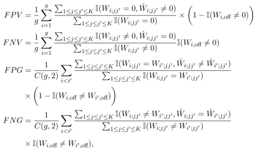
F P V = 1 g g X i=1 P 1≤j≤j0_≤_KI(Wi;jj0 = 0,Wˆ_i_;_jj0 6= 0) P 1≤j≤j0_≤_K_I(W_i_;_jj0 = 0) × 1−_I(Wi,off6= 0) F N V = 1 g g X i=1 P 1≤j≤j0_≤_K_I(W_i_;_jj0 6= 0,Wˆ_i_;_jj0 = 0) P 1≤j≤j0_≤_KI(Wi;jj0 6= 0) I (Wi,off6= 0) F P G= 1 C(g,2) X i<i0 P 1≤j≤j0_≤_K_I(W_i_;_jj0 =W_i0_;_jj0,Wˆ_i_;_jj0 6= ˆW_i0_;_jj0) P 1≤j≤j0_≤_K_I(W_i_;_jj0 =W_i0_;_jj0) × 1−_I(Wi,off6=Wi0_,_off) F N G= 1 C(g,2) X i<i0 P 1≤j≤j0_≤_K_I(W_i_;_jj0 6=W_i0_;_jj0,Wˆ_i_;_jj0 = ˆW_i0_;_jj0) P 1≤j≤j0_≤_KI(Wi;jj0 6=W_i0_;_jj0) ×_I(Wi,off6=Wi0_,_off),

whereC(g,2) is the combinatorial number of choosing 2 from g.

Table 2.1 shows the results for n = 173 based on 50 simulations for each set-up. With the true model as the fitted model by the method of Zhou et al. (2009), the method of Zhou et al. (2009) itself gave the highest Rand index, suggesting the best accuracy for clustering. However, It did not give the lowest average entropy loss (EL) and quadratic loss (QL) for precision matrix estimation, though the differences were not large. Recall that the true model here was based on four largely differing cluster-specific precision matrices, which might not favor fusing the cluster-specific precision matrices. Impressively our method New-SP gave the second highest Rand index that was quite close to that of Zhou et al. (2009), and more importantly, New-SP gave the most or second most accurate estimates of the cluster-specific precision matrices with the lowest average EL and second lowest QL. In addition, it also gave low false positive rates of sparseness and grouping, but high false negative rates. It is noted that New-JGL also performed well.

On the other hand, if the true model was the fitted one by New-SP, then New-SP was the clear winner for both clustering and precision matrix estimation, followed by New-JGL. This was the case when the cluster-specific precision matrices differed but sharing some commonalities. Finally, if the true model was the fitted one from New-JGL, the winners were New-JGL and New-SP, followed by mclust and the method of

(26)

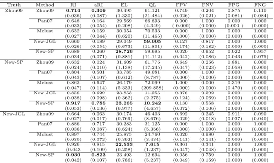
Truth Method RI aRI EL QL FPV FNV FPG FNG Zhou09 Zhou09 0.714 0.309 30.495 61.121 0.749 0.204 0.875 0.110 (0.036) (0.087) (1.330) (21.484) (0.026) (0.021) (0.081) (0.084) Pan07 0.648 0.164 29.569 66.893 0.000 1.000 0.000 1.000 (0.033) (0.054) (0.208) (4.349) ( 0.000) (0.000) (0.000 ) (0.000) Mclust 0.632 0.159 30.054 70.533 0.000 1.000 0.000 1.000 (0.027) (0.044) (0.620) (11.465) (0.000) (0.000) (0.000) (0.000) New-JGL 0.660 0.189 29.049 59.005 0.127 0.817 0.000 1.000 (0.026) (0.054) (0.673) (11.801) (0.174) (0.182) (0.000) (0.000) New-SP 0.689 0.260 28.726 59.695 0.020 0.952 0.022 0.957 (0.034) (0.071) (0.881) (11.112) (0.042) (0.086) (0.043) (0.075) New-SP Zhou09 0.632 0.024 31.609 61.775 0.649 0.256 0.881 0.000 (0.024) (0.010) (1.138) (17.245) (0.047) (0.023) (0.058) (0.000) Pan07 0.804 0.501 33.785 49.081 0.000 1.000 0.000 0.000 (0.043) (0.107) (0.612) (8.787) (0.000) (0.000) (0.000) (0.000) Mclust 0.862 0.647 26.179 72.099 1.000 0.000 0.319 0.000 (0.047) (0.114) (5.333) (209.858) (0.000) (0.000) (0.470) (0.000) New-JGL 0.856 0.629 23.853 11.255 0.376 0.292 0.000 0.000 (0.038) (0.098) (0.362) (2.275) (0.124) (0.069) (0.000) (0.000) New-SP 0.917 0.785 23.265 10.242 0.130 0.558 0.000 0.000 (0.053) (0.136) (0.977) (4.657) (0.072) (0.106) (0.000) (0.000) New-JGL Zhou09 0.664 0.063 30.174 46.403 0.692 0.245 0.911 0.090 (0.027) (0.017) (0.769) (8.676) (0.029) (0.018) (0.037) (0.040) Pan07 0.886 0.717 30.283 31.125 0.000 1.000 0.000 1.000 (0.036) (0.087) (0.624) (5.356) (0.000) (0.000) (0.000) (0.000) Mclust 0.897 0.744 25.875 24.760 0.020 0.980 0.000 1.000 (0.030) (0.072) (0.392) (3.434) (0.141) (0.141) (0.000) (0.000) New-JGL 0.926 0.815 22.533 7.615 0.361 0.341 0.000 1.000 (0.043 (0.109) (0.258) (1.237) (0.047) (0.048) (0.000) (0.000) New-SP 0.930 0.823 23.493 12.694 0.056 0.759 0.000 1.000 (0.042) (0.107) (0.786) (5.237) (0.049) (0.159) (0.000) (0.000)

Table 2.1: Simulation results with n= 173 and the true model being that estimated byone of the three methods based on the glioblastoma dataset. The means (standard deviations) of the Rand Index (RI), adjusted Rand Index (aRI), average entropy loss (EL) average quadratic loss (QL), average false positive for sparseness pursuit (FPV), average false negative for sparseness pursuit (FNV), average false positive for grouping (FPG) and average false negative for grouping (FNG) are shown for 50 simulations.

Pan and Shen (2007) (where a common diagonal precision matrix was assumed). We also investigated the sensitivity of the EM algorithm to its starting values. For the set-up with the true model as the one fitted by New-JGL, instead of using the K-means output as the starting value for New-JGL and New-SP, we used some randomly generated numbers as the starting value. The resulting Rand index values for New-JGL and New-SP decreased from 0.926 and 0.930 to 0.635 and 0.757 respectively, confirming the importance of using good starting values for the EM algorithm. However, the estimation errors for the precision matrices were less influenced: for example, the mean EL for New-JGL and New-SP increased from 22.533 and 23.493 to only 23.964 and 25.743, respectively, still lower than those of the other methods.

Next we doubled the sample size in simulations. With the increased sample size, the proposed method New-SP became the clear overall winner, followed by New-JGL

(27)

(Table 2.2). Although mclust performed well in the last two set-ups (with the true model being that fitted by New-SP or New-JGL), it did not work well in the first set-up. Again it is noted that the two new methods largely outperformed the method of Zhou et al. (2009) [12] for estimating the cluster-specific precision matrices, perhaps due to the former two’s use of the fusion penalties for information borrowing across multiple cluster-specific precision matrices.

2.4 Example

2.4.1 Glioblastoma Gene Expression Data

Verhaak et al. (2010) [1] studied a gene expression data set of glioblastoma tumor and normal samples. They used a consensus hierarchical clustering method to identify four disease subtypes. It is noted that, due to the limitation of the clustering method, the conditional dependencies between genes in each cluster were ignored and thus not revealed. This leaves room for our new and other methods to explore possible depen-dency relationships among the genes. Furthermore, the identified four clusters, albeit biologically reasonable, are in no way to be perfect, which bears importance when one uses their sample assignments as a reference to compare various methods.

To be practically focused, we restricted our analysis to the gene expression data from the 173 core samples as used by Verhaak et al.(2010) [1], and we selected only 20 genes that are related to cell signaling pathways. Some of these genes were demonstrated to be altered in Figure 4B in Brennan et al. (2013) [44] and Figure 5 in Mclendon et al. (2008) [45]. Specifically, genes EGFR, PDGFRA, FGFR3 are members of the RTK signaling pathway. RASGRP3 and RRAS are downstream targets of the RTK signaling pathway. PIK3C2B, PIK3R1, PIK3R3, PIK3IP1 and AKTIP are components of the PI3K/AKT signaling pathway. NFIB is the downstream target of RTK and PI3K/AKT signaling pathways. CDKN3, CDK4, CDKN1A, CDKN2C, CCND2 are involved in RB signaling pathways and they play important roles in cell cycle regulation. CASP1 and CASP4 are important genes in cell apoptosis.

(28)

2.4.2 Estimated networks

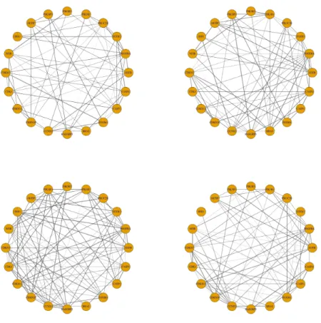
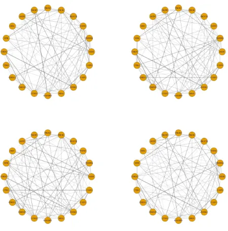
We applied our method New-SP to the glioblastoma gene expression data set. Trying with g = 1,2,3,4,5 clusters, it reached four clusters/subtypes. Each cluster showed a distinct conditional dependency structure among the genes, though their overall struc-tures were similar (Figure 2.1).

This suggests distinct cell signalling network changes across the disease subtypes. A closer examination of the estimated precision matrices reveals that the conditional dependencies among the receptor kinases and the downstream target genes were altered. The PI3K/Akt signaling pathway plays an important role in cell survival and prolifer-ation in glioblastoma ([46, 47]). One of the estimated networks shows that the AKTIP gene was conditionally correlated with CDKN2C, a gene encoding a cyclin-dependent kinase inhibitor that regulates cell growth. However, this link was lost in all other three estimated networks. Similarly, PIK3IP and AKTIP were not conditionally correlated with CDKN1A, CDKN2C and CDKN3 in one or more estimated networks, while the network in bottom left of Figure 2.1 preserved most of the connections. The PI3K/Akt signaling pathway is reported to be upstream of CCND2, a gene encoding the cell cy-cle regulating protein Cyclin D2 ([48]). Only one out of four subtypes demonstrated a conditional dependence between AKTIP and CCND2. The changes between these links collectively suggested dysregulation of cell growth by the PI3K/Akt signaling pathway in some subtypes of glioblastoma.

Gene IDH1 is known to have a higher mutation frequency in some glioblastoma subtypes, and here it exhibited cluster-specific associations with FGFR3, which was also reported to have mutations in glioblastoma subtypes classified by Verhaak et al. (2010) [1]. We found that gene IDH1’s expression was positively correlated with that of FGFR3 in only one cluster, suggesting possibly altered co-expressions in other clusters. IDH1 mutation is reported to cause widespread changes in histone and DNA methylation and potentially promoting tumorigenesis ([49, 50]). CCND2 was found to be amplified in IDH1 mutant medulloblastoma subtypes ([51]). Therefore, the abnormal IDH1 gene level and its disconnection with CCND2 observed in the estimated network pointed to possible roles of IDH1 in oncogenesis in certain subtypes of glioblastoma.

For comparison, we applied Zhou et al.’s method to the glioblastoma gene expression data set with cluster-specific covariance matrices. Among g = 1,2,3,4,5 clusters, it

(29)

Figure 2.1: Estimated cluster-specific networks based on 173 core samples using the new method New-SP.

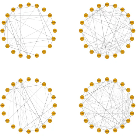
selected four clusters. The estimated cluster-specific precision matrices demonstrated cluster-specific dependencies among the genes (Figure 2.2). The estimated networks using Zhou et al.’s method confirmed that the conditional correlation between IDH1 and CCND2 was lost in one network estimated by the New-SP method. The conditional correlation between AKTIP and CCND2 was present in three subtypes, though the correlation was weak in one subtype. Compared to the networks estimated by the method of New-SP, the dependency changes across the clusters estimated by Zhou et al.’s method were much more dramatic, reflecting possibly large variations of the estimates without borrowing information across clusters.

(30)

Figure 2.2: Estimated cluster-specific networks based on 173 core samples using the method of Zhou et al. (2009).

estimated by the New-SP method, the networks estimated by the New-JGL method shared some structural similarity. The AKTIP and CCND2 correlation was found in two out of four subtypes, although the correlation in one subtype was weak. This agreed with the correlation in the networks estimated by the New-SP method. Unlike in Figure 2.1, the conditional correlation between IDH2 and CCND2 was present in all four subtypes, though the magnitude of correlation was small.

The non-penalized mclust yielded four clusters with a common covariance matrix, suggesting that the differences among the four cluster-specific covariance matrices were possibly subtle. This was also reflected from the overall similarity across the four cluster-specific estimates of the two new methods.

(31)

Figure 2.3: Estimated cluster-specific networks based on 173 core samples using the method of New-JGL.

2.4.3 Sample cluster assignments

Using the cluster assignments in Verhaak et al. (2010) [1] as the reference, the agreement between our New-SP method and the reference as measured by the Rand index was 0.747 and by the adjusted Rand index was 0.354 (Table 2.3). Its performance was compared with several other methods. First, the method of Pan and Shen (2007) [11] based on a common diagonal covariance matrix yielded 5 clusters with a Rand index of 0.749 and the adjusted Rand index of 0.358. For the purpose of comparison, we also examined the clustering results of the method by forcing 4 clusters, which led to a Rand index of 0.780 and the adjusted Rand index of 0.439 (Table 2.3). Although the method of Pan and Shen yielded a slightly higher Rand index, it was possibly due to the bias of

(32)

the reference clustering method (that ignored varying within-cluster dependencies that would in turn favor the results of Pan and Shen (2007)). More importantly, a common diagonal covariance matrix assumed and estimated by the method cannot be used to examine possibly varying within-cluster dependency structures. Finally, the two new methods seemed to perform better than the two other methods.

2.4.4 Model assessment

To check the goodness-of-fit of a final model, we propose using the parametric bootstrap, which was used by McLachlan and others to select the number of components in a Gaussian mixture model ([52, 53]). For example, for our real data, the New-SP method selected a final model with four components, each with a component-specific precision matrix, which is called an alternative model here; it may be of interest to compare this alternative model with a null (or reduced) model with four components but a common precision matrix, which could be achieved by forcing a largeλ2 value (while other tuning

parameters were selected as before). We generated 50 bootstrap samples from the fitted null and alternative models respectively, then fitted the two models respectively to the bootstrap samples; finally, we compared their corresponding CV log-likelihood values, as shown in Figure 2.4. For the bootstrap samples, in both cases fitting the alternative model seemed to yield a higher mean value of the CV log-likelihood; however, the difference between the two fitted models was larger when the bootstrap samples were generated from the alternative model, as expected. Since the CV log-likelihood value difference between the two fitted models based on the original data was larger than that from the bootstrap samples generated from the alternative model, there was some evidence to support the use of the alternative model. Nevertheless, perhaps due to the relatively small sample sizes and shrinkage effects of the four component-specific precision matrices towards each other (as imposed by the fusion penalty even in the alternative model), the difference between the two models was not overwhelming, and cautions must be taken in not over-interpreting their differences.

(33)

Null−Null Null−Alt Alt−Null Alt−Alt −1950 −1900 −1850 −1800 Null log−likelihood Alt log−likelihood

Figure 2.4: Distributions of the CV log-likelihood values of various fitted models based on bootstrap samples. Null-Null, bootstrap samples were generated from the null model, to which the null model was fitted; Null-Alt, bootstrap samples were generated from the null model, to which the alternative model was fitted; Alt-Null, bootstrap samples were generated from the alternative model, to which the null model was fitted; Alt-Alt, bootstrap samples were generated from the alternative model, to which the alternative model was fitted. The two horizontal lines are the CV log-likelihood values for the two fitted models to the original data.

2.5 Discussion

We have presented a new approach to estimation of multiple networks in the context of a penalized Gaussian mixture model. The primary goal is for estimating and comparing cluster-specific network changes, though automatic cluster discovery is often of interest too. For the primary goal, it is necessary to encourage the equalities of the entries across the cluster-specific precision matrices while maintaining their differences if any, which is best accomplished by fusion with a non-convex penalty such as TLP as adopted in our proposed method New-SP ([43], [9]). Note that standard and existing penalized model-based clustering methods are not suitable for our primary goal: due to the lack of fusion penalties, the existing methods cannot highlight few major differneces across multiple precision matrix estimates, in addition to their loss of estimation efficiency

(34)

without information borrowing. Both our proposed methods pursue both sparseness and fusion for multiple precision matrices in the framework of Gaussian mixture modeling. Our approach takes advantage of the existing methods using convex or non-convex penalties to regularize the parameters in the unconstrained precision matrices based on Gaussian graphical models, which assumes that it is known that which samples are from which Gaussian distributions, differing from our current context with unknown sample heterogeneity.

We applied the methods to a real data set containing gene expression profiles of glioblastoma patients. Using the New-SP method, the samples were partitioned into four disease subtypes, as reported in Verhaak et al. (2010) but based on only differential gene expression. Importantly, our method reconstructed disease subtype-specific gene networks, suggesting candidates for possibly subtype-specific gene dysregulations that can be followed up in further biological experiments. Since the truth is unknown for the real data, we recoursed to realistic simulations mimicking the real data to evaluate the methods; it was demonstrated that our method New-SP based on the non-convex TLP gave the best overall performance in both clustering (i.e. subtype discovery) and network estimation when the sample size was at least moderately large, followed by the other proposed method New-JGL based on the convex (fused) Lasso penalty. The better performance of New-SP over New-JGL is likely due to the non-convex TLP adopted in the former, as demonstrated in Shen et al. (2012) [43] for regression and single precision matrix estimation and Zhu et al. (2014) [9] for estimating multiple precision matrices in Gaussian graphical models. On the other hand, New-JGL is simpler and faster than New-SP, and thus can be used for larger problems and/or to provide a quick preliminary solution; in particular, we advocate using the results of New-JGL (or any other method with a convex penalty) as a good starting value for New-SP, thus the latter can be regarded as a refinement of the former. We also note that partition rules discussed in Zhu et al. (2014) can be used to speed up the new methods for high-dimensional data. We emphasize that the existing methods for estimation of multiple networks, in-cluding the two used here (Danaher et al. 2014; Zhu et al. 2014 [3, 9]), are based on Gaussian graphical models without sample heterogeneity; that is, each sample is assumed to be known from a given Gaussian distribution. In our target applications and other settings, this sample homogeneity assumption may not hold. For example, in

(35)

clinical genomic studies, due to disease heterogeneity, the assumption that all the gene expression profiles of cancer patients come from the same Gaussian distribution is not practical. To discover unknown disease subtypes, clustering or unsupervised learning becomes useful, which will facilitate personalized medicine. To our knowledge, exist-ing clusterexist-ing methods of gene expression have focused on detectexist-ing differential mean expression levels across clusters or disease subtypes, as demonstrated in Verhaak et al. (2010) [1]. However, in addition to differential gene expression, there are possibly dif-ferential gene regulations or dysregulations across disease subtypes. If disease subtypes are known, then differential gene regulations can be treated as estimating multiple pre-cision matrices in Gaussian graphical models, as handled by many existing methods; otherwise, as discussed here, both disease subtypes and possibly differential precision matrices must be inferred simultaneously based on a Gaussian mixture model.

Our methods are implemented in an R package pGMM that will be available on CRAN.

Acknowledgment

The authors are grateful to the Editor and reviewers for constructive comments. This research was supported by NIH grants R01GM081535, R01GM113250, R01HL105397 and R01HL116720, and by the Minnesota Supercomputing Institute.

(36)

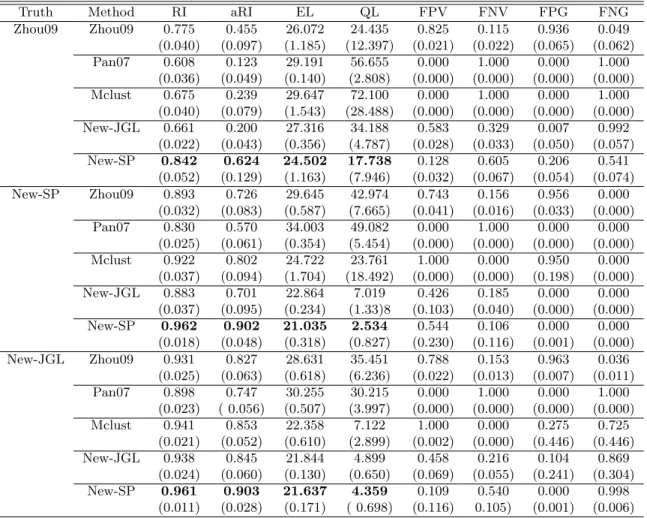
Truth Method RI aRI EL QL FPV FNV FPG FNG Zhou09 Zhou09 0.775 0.455 26.072 24.435 0.825 0.115 0.936 0.049 (0.040) (0.097) (1.185) (12.397) (0.021) (0.022) (0.065) (0.062) Pan07 0.608 0.123 29.191 56.655 0.000 1.000 0.000 1.000 (0.036) (0.049) (0.140) (2.808) (0.000) (0.000) (0.000) (0.000) Mclust 0.675 0.239 29.647 72.100 0.000 1.000 0.000 1.000 (0.040) (0.079) (1.543) (28.488) (0.000) (0.000) (0.000) (0.000) New-JGL 0.661 0.200 27.316 34.188 0.583 0.329 0.007 0.992 (0.022) (0.043) (0.356) (4.787) (0.028) (0.033) (0.050) (0.057) New-SP 0.842 0.624 24.502 17.738 0.128 0.605 0.206 0.541 (0.052) (0.129) (1.163) (7.946) (0.032) (0.067) (0.054) (0.074) New-SP Zhou09 0.893 0.726 29.645 42.974 0.743 0.156 0.956 0.000 (0.032) (0.083) (0.587) (7.665) (0.041) (0.016) (0.033) (0.000) Pan07 0.830 0.570 34.003 49.082 0.000 1.000 0.000 0.000 (0.025) (0.061) (0.354) (5.454) (0.000) (0.000) (0.000) (0.000) Mclust 0.922 0.802 24.722 23.761 1.000 0.000 0.950 0.000 (0.037) (0.094) (1.704) (18.492) (0.000) (0.000) (0.198) (0.000) New-JGL 0.883 0.701 22.864 7.019 0.426 0.185 0.000 0.000 (0.037) (0.095) (0.234) (1.33)8 (0.103) (0.040) (0.000) (0.000) New-SP 0.962 0.902 21.035 2.534 0.544 0.106 0.000 0.000 (0.018) (0.048) (0.318) (0.827) (0.230) (0.116) (0.001) (0.000) New-JGL Zhou09 0.931 0.827 28.631 35.451 0.788 0.153 0.963 0.036 (0.025) (0.063) (0.618) (6.236) (0.022) (0.013) (0.007) (0.011) Pan07 0.898 0.747 30.255 30.215 0.000 1.000 0.000 1.000 (0.023) ( 0.056) (0.507) (3.997) (0.000) (0.000) (0.000) (0.000) Mclust 0.941 0.853 22.358 7.122 1.000 0.000 0.275 0.725 (0.021) (0.052) (0.610) (2.899) (0.002) (0.000) (0.446) (0.446) New-JGL 0.938 0.845 21.844 4.899 0.458 0.216 0.104 0.869 (0.024) (0.060) (0.130) (0.650) (0.069) (0.055) (0.241) (0.304) New-SP 0.961 0.903 21.637 4.359 0.109 0.540 0.000 0.998 (0.011) (0.028) (0.171) ( 0.698) (0.116) 0.105) (0.001) (0.006)

Table 2.2: Simulation results with n= 346 and the true model being that estimated byone of the three methods based on the glioblastoma dataset. The means (standard deviations) of the Rand Index (RI), adjusted Rand Index (aRI), average entropy loss (EL) average quadratic loss (QL), average false positive for sparseness pursuit (FPV), average false negative for sparseness pursuit (FNV), average false positive for grouping (FPG) and average false negative for grouping (FNG) are shown for 50 simulations.

(37)

New-SP mclust Pan07 Zhou09 New-JGL

p= 20 RI 0.747 0.688 0.780 0.713 0.746

aRI 0.354 0.222 0.439 0.305 0.355

Table 2.3: Rand Index (RI) and adjusted Rand Index (aRI) for the glioblastoma gene expression data with 20 genes by various methods. The class assignments given in [1] are used as the reference.

(38)

Chapter 3

ADAPTIVE TESTING OF

SNP-BRAIN FUNCTIONAL

CONNECTIVITY

ASSOCIATION VIA A

MODULAR NETWORK

ANALYSIS

3.1 Introduction

Resting-state functional magnetic resonance imaging (rs-fMRI) is gaining popularity in studies of brain functional connectivity with applications to detection of subtle network reorganizations in Alzheimer’s disease [54]. Disruption of connectivity in the brain functional network is related to many pathological conditions in the brain, such as Alzheimer’s disease [55], schizophrenia [15], or autism [17]. This necessitates the devel-opment of methods for modelling the brain functional network its statistical inference. A network is comprised of nodes and edges connecting the nodes. Based on func-tional MRI data, a popular choice of nodes are brain regions of interest (ROIs) while the

(39)

edges are connectivities reflecting statistical dependencies between ROIs. An important network model, the scale-free network[56], assumes that most nodes in a network are sparsely connected with the exception of a few “hub” nodes that are densely connected with other nodes. In the scale-free network model, new connections are more likely to occur for those hub nodes with already-high connectivity. There has been empirical evidence supporting this model for brain functional networks [57], though it is still de-batable. In addition, the scale-free network model also admits a modular topological structure, which can be extracted for more efficient analyses for human brains.

Methods for drawing statistical inference to distinguish brain connectivity for dif-ferent groups of subjects are still under development. The first question encountered is how to define brain functional connectivity. Ref. [58] discussed the choice between Pearson’s marginal correlation coefficient and partial correlation coefficient as a network connectivity measure, though other measures are possible and it is yet unclear which one is best. To reduce dimensionality and to reach sparseness, graphical lasso is often used for estimating networks for different groups. Since an estimated network with the imposed sparsity penalty may not demonstrate modular structures, a better approach is to directly discover the modules in a network. A general framework for estimating scale-free networks and detecting modules is proposed in Ref. [20] for gene network anal-ysis, which has gained tremendous popularity in genomics [59]. It starts by defining a similarity measure between two nodes in a network, called adjacency, using the marginal correlation coefficient. Soft-thresholding is then applied, leading to a weighted network. The soft-thresholded adjacency is further transformed to a topological overlap matrix (TOM) element, which is converted to a dissimilarity measure for hierarchical cluster-ing, grouping closely connected nodes together as modules in the network. The above framework not only provides multiple network connectivity measures, but also carries out modular structure identification. The connectivity measures and identified mod-ules in the brain functional network may help statistical inference and offer biological insights [59].

In this paper, for the first time, we adapt the use of WGCNA for gene expression data to rs-fMRI data, constructing weighted brain functional networks and identifying their subnetworks or modules using the Alzheimer’s Disease Neuroimaging Initiative (ADNI) data. We explored using the adjacency matrix element and TOM element, in

(40)

addition to the marginal correlation or covariance, to characterize connectivity in brain functional networks. Taking advantages of detected network modules, we conduct asso-ciation analysis of genetic variants with not only the whole brain functional network, but also its various subcomponents, including its modules, which aims to not only improve statistical power, but also offer better biological interpretation. We propose applying a new adaptive association test based on a proportional odds model (POM) accounting for the ordinal nature of the SNP genotype. We found evidence of associations between several network modules and the APOE4 variant, which is by far the most significant genetic risk factor for Alzheimer’s disease.

This paper is organized as follows. We first review the method of WGCNA, includ-ing its module identification, then introduce the adaptive test based on a POM. We demonstrate the application of our methods to the ADNI data before summarizing our findings and future research directions in the discussion section.

3.2 Methods

3.2.1 Module detection via weighted gene co-expression network anal-ysis

In this section, we briefly review the work in Ref. [20] on the weighted gene-coexpression network analysis (WGCNA) framework for network construction and module identifi-cation.

Adjacency matrix

The first step of the WGCNA framework is to define a similarity measure between gene expression profiles; in the current context, we use the BOLD signals in each of multiple ROIs from one or more subjects to calculate a similarity between any two ROIs. The similarity measure is required to take values between 0 and 1. A typical choice of this similarity measure is the absolute value of the Pearson correlation coefficient suv =

|cor(u, v)|, for nodes u and v. Another choice, which preserves the sign of correlation, is defined as suv = [1 +cor(u, v)]/2. We refer the first one as unsigned similarity

(41)

applications to the ADNI data, the identified modules have negligible differences using either unsigned or signed similarity measure. We used the unsigned similarity measure throughout this paper.

Once the similarity measure is computed, the next step is to transform the simi-larity matrix S = [suv] into an adjacency matrix using an adjacency function. Hard

thresholding is often used to yield a binary or unweighted network with a 0/1 adjacency indicating no-connection/connection and thus possible loss of information, though a more efficient multi-scale approach with multiple thresholds yielding a set of binary networks has been proposed [60]. Soft thresholding is a simple and popular alternative with more flexibilities. One choice is the power adjacency function

auv=power(suv, δ)≡ |suv|δ (3.1)

with parameterδ, which is chosen as the smallest integer such that the scale-free network model fitting is above a certain threshold.

Topological overlap matrix

Instead of using only the adjacency matrix, Ref. [61] advocated a topological overlap matrix Ω = [ωuv] with its element as a potentially more useful measure that reflects

the relative interconnectedness of two nodes u and v after accounting for their shared neighbors. The topological overlap matrix element is defined as

ωuv =

luv+auv

min{ku, kv}+ 1−auv

(3.2)

with ku = P_vauv and luv = P_qauqaqv. For a binary network with auv = 0 or 1, ku

is the connectivity of node u representing the number of its direct neighbors, while luv

equals the number of nodes that connect both nodes u and v; ωuv = 0 if the nodes u

and vare not connected and they are not connected to the same neighbors; in contrast,

ωuv = 1 if the nodes u and v are connected and the neighbors of the node with fewer

edges are also connected to the one with more edges. For any network, 0 ≤ auv ≤ 1

(42)

Module identification

To identify modules in a network, we need to have a dissimilarity or distance measure. An intuitive way is to convert a similarity measure. Based on the topological overlap matrix element ωuv, we can simply define the dissimilarity measure as dωuv = 1−ωuv.

The TOM-based dissimilarity dω_uv is used as the input for average linkage hierarchi-cal clustering. The output from hierarchihierarchi-cal clustering is a dendrogram composed of branches and leaves. In a brain functional network, each leaf corresponds to a ROI. The hierarchical clustering algorithm groups the closest ROIs and forms the branches. By cutting the branches of the dendrogram, closely related ROIs are identified as a module. Among the several methods for cutting the branches of the dendrogram, the default used in the WGCNA framework is Dynamic Tree Cut from the R package dynamicTreeCut.

Once modules are identified, one can calculate an intramodular connectivity

ω.inu =

X

v∈M

ωuv (3.3)

for each nodeuin its moduleM. Ref. [20] pointed out that intramodular connectivities

ω.in may represent important features of the nodes (i.e. ROIs).

3.2.2 An adaptive association test based on the proportional odds model

Let Yi = 0,1,2 denote the count of the minor allele for subject i for a given SNP of

interest, then Yi hasJ = 3 ordered categories. The logistic regression model cannot be

applied in this situation, because it only allows the response variable to be binary. A popular choice for ordinal data is the proportional odds model (POM)[62], which we will briefly describe here.

Suppose subject i has p network connectivities denoted by Xi = (xi1, . . . , xip) and

l covariates denoted by Zi = (zi1, . . . , zil). For the proportional odds model, we define

the regression coefficients β = (β1, . . . , βp)0 for the network connectivities and δ =

(δ1, . . . , δl)0, and a vector of intercepts α = (α0, . . . , αJ−2)0. The proportional odds

model is

(43)

The likelihood for equation Eq. 3.4 can be derived based on the multinomial distribution for the categorical variableYi, from which maximum likelihood estimates and statistical

inference can be obtained as implemented in R packageMASSorVGAM. However, numer-ical issues such as non-convergence arise whenp, the dimension ofβ, is relatively large as compared to the sample size n.

Here we propose applying a class of tests that are applicable to the high-dimensional setting withp > n, from which an adaptive test is constructed to summarize information across the tests. No that most existing tests cannot be applied to the case p > n. To test the null hypothesis H0 : β = (β1, β2, . . . , βp)0 = 0, we can use the score vector

derived in Ref. [21], Uβ = n X i=1 J−2 X j=0 (1−rˆi(j−1)−rˆij)·I(Yi =j)·Xi (3.5)

where ˆrij = exp( ˆα+Ziδˆ)/[1 + exp( ˆα+Ziˆδ)] comes from the fitted null model of Eq. 3.4

(i.e. with β = 0); ˆα and ˆδ are estimated by the polr function in the R package MASS. Let Uk denote thekth component of the score vector Uβ = (U1, . . . , Up)0. The SPU(γ)

test statistic is defined as

TSP U(γ)=

p

X

k=1

U_kγ, (3.6)

where γ ≥ 1 is an integer. As the parameter γ increases, a connectivity with a larger absolute value of the score gains a higher weight. In the extreme situation, whenγ → ∞

as an even integer, SP U(∞) takes only the maximum component of the score vector, i.e., T_{SP U}₍∞)= max

p

k=1|Uk|.

The p-values of the SPU tests are computed by permuting the residuals from the null model B times, and the p-value can be calculated as

PSP U(γ)= (PB b=1I[|T (b) SP U(γ)| ≥ |TSP U(γ)|] + 1) (B+ 1) , (3.7)

whereT_{SP U}(b) ₍_γ₎ is the SPU(γ) statistic based on thebth set of permuted residuals. Since the value ofγthat yields highest power cannot be determined a priori, an adaptive SPU (aSPU) test is introduced to combine the evidence across multiple SPU tests,

TaSP U = min