Time series forecasting by principal covariate regression
Christiaan Heij
∗, Patrick J.F. Groenen, Dick J. van Dijk
Econometric Institute, Erasmus University Rotterdam
Econometric Institute Report EI2006-37
31-08-2006
Abstract
This paper is concerned with time series forecasting in the presence of a large number of predictors. The results are of interest, for instance, in macroeconomic and financial forecasting where often many potential predictor variables are available. Most of the current forecast methods with many predictors consist of two steps, where the large set of predictors is first summarized by means of a limited number of factors —for instance, principal components— and, in a second step, these factors and their lags are used for forecasting. A possible disadvantage of these methods is that the construction of the components in the first step is not directly related to their use in forecasting in the second step. This motivates an alternative method, principal covariate regression (PCovR), where the two steps are combined in a single criterion. This method has been analyzed before within the framework of multivariate regression models. Moti-vated by the needs of macroeconomic time series forecasting, this paper discusses two adjustments of standard PCovR that are necessary to allow for lagged factors and for preferential predictors. The resulting nonlinear estimation problem is solved by means of a method based on iterative majorization. The paper discusses some numerical aspects and analyzes the method by means of simulations. Further, the empirical per-formance of PCovR is compared with that of the two-step principal component method by applying both methods to forecast four US macroeconomic time series from a set of 132 predictors, using the data set of Stock and Watson (2005).
Keywords
principal covariate regression, economic forecasting, dynamic factor models, principal components, distributed lags, iterative majorization
1
Introduction
Econometric modelers face many decisions, as was recently discussed in the special ‘Collo-quium for ET’s 20th Anniversary’ issue of this journal by, among others, Hansen (2005), Pesaran and Timmermann (2005), and Phillips (2005). In this paper, we pay attention to one of the basic questions in forecasting, that is, which information should be included in the model. In many cases, observational data are available for a large number of predictor vari-ables that may all help to forecast the variable of interest. To exploit such rich information, one should somehow limit the model complexity, as otherwise the forecasts will suffer from overfitting due to the well-known curse of dimensionality. For instance, if T observations are available for a set ofk predictors, then fork > T it is simply impossible to estimate a multiple regression model involving all predictors as separate regressors. Ifk is large with k ≤T, then it is still not advisable to estimate a regression model with all predictors as regressors because the resulting forecasts will have large variance due to overfitting. Better forecasts may be achieved by compressing the information in the predictors somehow and by using a forecast equation containing fewer predictors.
Several methods for forecasting with many predictors have been proposed in the liter-ature. We refer to Stock and Watson (in press) for a survey. For instance, in ‘principal component regression’ (PCR) the information in thek predictors is summarized by means of a relatively small number of factors (the principal components) and these factors are used as predictors in a low-dimensional multiple regression model. This approach is based on dynamic factor models and is followed, for instance, by Stock and Watson (1999, 2002a,b, 2005) to forecast key macroeconomic variables from large sets of predictor variables. An essential aspect of PCR and similar methods is that they consist of two stages, that is, first the factors are constructed and then the forecast equation is estimated.
The goal of this paper is to analyze a method that combines the two stages of predictor compression and forecasting in a single criterion. This method, called principal covariate regression (PCovR), was proposed by De Jong and Kiers (1992) for multiple regression mod-els. PCovR is a data-based method that does not employ an explicit underlying statistical model. Therefore, we will follow a data analysis approach in our paper and we will not assume a statistical model for the data.
In Heij, Groenen, and Van Dijk (2005), the forecast performance of PCovR and PCR was compared for simple forecast models that employ only the current factors and not their lags. In the current paper, we extend the PCovR method in two respects that are essential for practical applications in economics. The first extension is to allow for preferential pre-dictors, that is, predictors that are always included in the forecast equation, for instance, because of their exceptional forecast power or their economic interpretation. This extension
is relatively straightforward, as the effects of the preferential predictors and of the factors can be estimated in an iterative way. The second extension is to allow for lagged factors in the prediction equation, which is relevant if the effect of the economic predictors is distributed over several periods of time. This extension is much more fundamental, as it requires non-linear estimation methods to respect the condition that the constructed lagged factors all originate from the same underlying factors. We propose an iterative majorization algorithm to estimate the model parameters. We also discuss some numerical aspects of PCovR, that is, the non-convexity of the PCovR criterion function, the issue of initial estimates, and the choice of weight factors in the PCovR criterion.
The forecast performance of PCovR is studied by means of simulation experiments. We investigate various factors that may affect the forecast performance, including the use of preferential predictors, the number of time lags, the number of predictors, and the correlation of the predictors with the variable to be predicted. We make also an empirical comparison of PCovR and PCR by forecasting four key variables of the real US economy (production, income, employment and manufacturing sales) from a set of 132 predictors, using the data set of Stock and Watson (2005). The forecast quality is evaluated by means of the mean squared (several periods ahead, out of sample) forecast error. We consider both single factor and multiple factor models. Model selection is based on the Bayes information criterion, as is common in PCR because of the work of Stock and Watson (1999, 2002a, 2002b, 2005), and also on cross validation methods.
The paper is organized as follows. In Section 2, we formulate the forecasting problem with compressed predictors in more detail and we describe the principal component method. In Section 3, we describe the PCovR method and we present estimation algorithms and discuss some numerical issues, in particular, the choice of PCovR weights. The performance of PCovR under various conditions is analyzed in Section 4 by means of simulation experiments, and Section 5 provides an empirical comparison of PCovR and PCR in macroeconomic forecasting. Section 6 concludes with a brief overview and with some suggestions for further research. Finally, technical results are treated in appendices.
2
Forecasting with compressed predictors
2.1
The forecast model
First we introduce some notation. The observations consist of time series of lengthT on a variable to be predicted (y) and on a set of predictor variables (X) and preferential predictors (Z; these variables are excluded fromX). We will always assume that the constant term is excluded both fromX and fromZ. Letk be the number of predictors andkz the number
matrix.
The idea is to summarize the information in thekvariablesX by means ofpfactorsF, withp(much) smaller thank. HereF is aT×pmatrix consisting of linear combinations of theX variables, so that
F =XA
for somek×pmatrixA. These factors are used, together with the preferential predictors, to forecastyby means of a distributed lag model. Ifqlags ofF andrlags ofZare incorporated in the model then the (one-step-ahead) forecast equation foryT+1 at periodT is written as
ˆ yT+1=α+ q X j=0 fT−jβj+ r X j=0 zT−jγj. (1)
Here α is the constant term, βj are p×1 vectors (j = 0, . . . , q), γj are kz×1 vectors
(j = 0, . . . , r), andfT−j=xT−jAwherextdenotes the 1×kvector of observations on the
predictors at timet. The (multi) h-step-ahead forecast equation has the same structure, replacing ˆyT+1 in (1) by ˆyT+h. In the sequel, we mostly consider the caseh= 1, but the
methods are easily extended forh >1. In the empirical application in Section 5, the forecast horizon ish= 12 months.
To apply the forecast model (1) in practice, we should choose the structure parameters (p, q, r) and estimate the parameters (A, α, β0, . . . , βq, γ0, . . . , γr) of the forecast equation.
In this paper, we pay most attention to the estimation of the parameters for a given set of structure parameters. However, in the simulation experiments in Section 4, we consider the effects of misspecification of (p, q, r), and in Sections 4 and 5 we consider the forecast per-formance if the structure parameters (p, q, r) are selected by the Bayes information criterion or by cross validation.
2.2
Two-step principal component regression (PCR)
In this section, we briefly describe the method of principal component regression (PCR) to estimate the forecast equation (1). We refer to Stock and Watson (1999, 2002a,b, 2005) for more details and for applications in macroeconomic forecasting.
The PCR method consists of two estimation steps. In the first step, A is estimated by means of principal components. That is, the pfactors are obtained by minimizing the squared Frobenius norm||X −Xˆ||2 under the restriction that ˆX has rankp. The squared
Frobenius norm of a matrix is simply the sum of squares of all elements of the matrix. TheX-variables should be standardized to prevent scale effects. For instance, each column (variable) ofX is scaled to have zero mean and unit norm.
The estimates A can be obtained from the singular value decomposition (SVD) of X. More precisely, letX =U SV0 be an SVD of X where the singular values in the diagonal
matrixSare listed in decreasing order. Then ˆX =UpSpVp0 whereUp andVp consist
respec-tively of the firstpcolumns ofU andV and whereSpis thep×pdiagonal matrix with thep
largest (non-zero) singular values ofX on the diagonal. Define thek×pmatrixA=VpSp−1
andp×k matrixB=SpVp0, then ˆX =XAB and (A, B) provides the minimizing solution
of
||X−XAB||2, withA k×p and B p×k. (2)
It is easily checked that the factors F = XA satisfy F0F = A0X0XA = I
p, so that the
p factors in F are scaled and mutually orthogonal. The factors F = XA are called the principal components ofX.
In the second step, the parameters (α, β0, . . . , βq, γ0, . . . , γr) in (1) are estimated by least
squares (OLS), for given values of A. Let F = XA with corresponding lagged matrices F(−1), . . . , F(−q), and letZ(−1), . . . , Z(−r) be the lagged matrices ofZ. Then the second step corresponds to minimizing
||y−α− q X j=0 F(−j)βj− r X j=0 Z(−j)γj||2, (3)
where some initial observations —that is, the first max(q, r) ones— should be dropped because of missing observations for the lagged terms ofF andZ.
Summarizing, PCR consists of the (SVD) minimization (2) followed by the (OLS) mini-mization (3). In the next section, we consider a method that integrates these two steps by minimizing a single criterion function.
3
Principal covariate regression (PCovR)
3.1
Introduction
In this section, we consider a method for forecasting with many predictors that combines the two stages of predictor compression and estimating the parameters of the forecast equation into a single criterion. This method is called ‘Principal Covariate Regression’ (PCovR) and was proposed by De Jong and Kiers (1992) within the framework of multiple regression models. We first describe ‘standard’ PCovR and we discuss extensions with preferential predictors in Section 3.2 and with lagged factors in Section 3.3.
In PCovR, the parameters are estimated by minimizing a weighted average of the forecast errors (3) (without preferential predictorsZ and without lags ofF, so that q= 0) and of the predictor compression errors (2). For given weightsw1 >0 and w2 >0 and for given
number of factorsp, the criterion to be minimized is
where theT×pmatrixF =XAconsists ofpfactors that compress the predictor information in theT ×k matrix X. As before, A is a k×pmatrix of rankp, B is a p×k matrix, α is a scalar and β is a p×1 vector. Clearly, if (A, B, α, β) is an optimal set of coefficients then (AR, R−1B, α, R−1β) is also optimal for every invertiblep×pmatrixR. Therefore,A
may be chosen such thatF0F =A0X0XA=I
p, asp≤rank(X). With this restriction, the
parameters are identified up to an orthogonal transformationR, that is, withR0R=I
p.
The vector norm in (4) is the Euclidean norm and the matrix norm is the Frobenius norm. To prevent scaling effects of theX-variables, we will assume that all variables —that is, all columns ofX— are scaled to have mean zero and norm one. Further, because only the relative weightw1/w2 is of importance, we consider weights of the form
w1= w
||y||2, w2=
1−w
||X||2, (5)
with 0≤w≤1. For scaled predictor data there holds||X||2=k, wherek is the number of
predictor variables. The user has to choose the PCovR weightw, balancing the objectives of good predictor compression forX (forwsmall) and good (in-sample) fit fory(forwlarge). The parameterw should be chosen between 0 and 1, because otherwise the criterion (4) becomes unbounded and has no optimal solution. If the weightw tends to 0 then PCovR converges to Principal Components (step 1 in PCR), and if w tends to 1 then PCovR converges to OLS.
The minimization of (4) is a nonlinear —in fact, bilinear— optimization problem, because of the product termsAβand AB. The estimates can be obtained by means of two SVD’s, see Heij, Groenen, and Van Dijk (2005). We refer to De Jong and Kiers (1992) for further background on PCovR in multiple regression models. The next two subsections discuss two extensions that are needed in time series forecasting, namely, the inclusion of preferential predictors and of lags in the forecast equation (1).
3.2
PCovR with preferential predictors
In many cases, one wishes to include some of the variables explicitly in the forecast equation, and not indirectly via the constructed factors. For instance, to predicty one may wish to use lagged values of y or variables closely related to y, and possibly also some variables suggested by (economic) theory. These preferential predictors are denoted by Z in the forecast equation (1). If we assume that there are no lags, so thatq =r= 0 in (1), then the PCovR criterion with preferential predictors is given by
f(A, B, α, β, γ) =w1||y−α−XAβ−Zγ||2+w2||X−XAB||2, (6)
A simple, alternating least squares method to estimate (A, B, α, β, γ) is the following. In Step 1, regressy on a constant and Z to get initial estimatesa ofαandc ofγ. In Step 2, use the residuals (y−a−Zc) andX to estimate (A, B, β) by standard PCovR as described in the foregoing section. These steps can be iterated, where at each new iteration updates of the estimates ofαandγare obtained by regressingy−XAbˆ on a constant andZ, where ˆA andbare the estimates ofAandβ obtained in the previous iteration. At each iteration and at both steps, the criterion valuef(A, B, α, β, γ) in (6) decreases and therefore converges, since it is bounded from below by zero.
3.3
PCovR with lagged factors
The methods discussed so far are too limited to deal with time series data, as the effect of the predictorsX andZonywill often be distributed over several time periods. Such distributed effects may occur, for instance, in macroeconomic applications where adjustments may be relatively slow. In such situations it is useful to incorporate lags in the forecast equation, as in (1) withqlags ofX andrlags ofZ.
Lags of preferential predictors can be incorporated simply by extending the matrix Z with additional columns for the lagged terms, so that Z in (6) is replaced by Zr =
[Z Z(−1) . . . Z(−r)]. In principle, one possible solution to add lagged factor terms is to extend also the original predictor matrixX with lagged terms, so thatX in (6) is replaced byXq = [X X(−1) . . . X(−q)]. The advantage is that the parameters can be estimated
in a relatively simple way. However, this method has three important disadvantages. The first objection is of a practical nature. The motivation for the predictor compression is that the number of predictorsk in X is relatively large. However, this dimensionality problem is magnified if we use Xq, as this matrix has k(q+ 1) columns instead of k. The second
objection is related to the interpretation of the constructed factors. IfF =XA, then at time t thepfactor values Ft=XtA consist of linear combinations of the values of the original
predictor variables that are all observed at the same time t. However, factors Fq = XqA
consist of mixtures of variables measured at different points in time, which makes it more difficult to interpret the factors. The third objection is that a large number of predictors requires the use of relatively small values for the weight factorw, as will be explained in Section 3.5. AsXq has much more columns thanX, the weight should be decreased
accord-ingly. In this case, the relative importance of the (in-sample) fit ofy in (4), (6) decreases, which may be a disadvantage in forecastingy.
Because of these considerations, we consider the PCovR criterion that is based directly on the forecast equation (3). The criterion is given byf =f(A, B, α, β0, . . . , βq, γ0, . . . , γr)
with f = w1||y−α− q X j=0 F(−j)βj− r X j=0 Z(−j)γj||2+w2||X−F B||2 = w1||y−α− q X j=0 (XA)(−j)βj− r X j=0 Z(−j)γj||2+w2||X−XAB||2, (7)
whereF =XAare the factors to be constructed and F(−j) = (XA)(−j) and Z(−j) are lags of respectivelyF=F(0) =XAandZ =Z(0). We include a constant termαin (7) to allow for possible non-zero sample means of the variables and their lags.
An advantage of this method is that the constructed factors have the usual interpretation of linear combinations of economic variables measured at the same point in time. A com-putational disadvantage is that the minimization of (7) can no longer be solved by SVD’s because of the implicit parameter restrictions for the parameters ofX, X(−1), . . . , X(−q) in (7). The resulting minimization problem can be solved by an iterative approximation method known as ‘iterative majorization’. This approach is discussed in general terms in the next subsection, and further details are given in Appendix A.1.
3.4
Iterative majorization for PCovR with lagged factors
The idea to solve the nonlinear minimization problem (7) is to approximate the criterion function by a simpler (quadratic) one that can be solved by SVD, and to iterate the approx-imation to get closer and closer to the minimum of the original criterion function (7). In this section, we give a general outline of the method, and details of the algorithm are given Ap-pendix A.1. For more background on iterative majorization we refer to Kiers (1990, 2002), De Leeuw (1994), Heiser (1995), Lange, Hunter and Yang (2000), and Borg and Groenen (2005).
Note that the non-linearity is only due to the parameter matrixA. Indeed, ifA is fixed thenF =XAand its lags are known, so that the parameters (α, β0, . . . , βq, γ0, . . . , γr) in
(7) can be estimated by regressingy on a constant and F and Z and their lags, and (each column of)B can be estimated by regressing (each column of) F onX. These regression estimates depend onA, and if we substitute the estimates in (7) then PCovR boils down to minimizing a non-linear functionf(A) of thek×pmatrixA, which is normalized so that A0X0XA=I
p.
The idea of majorization is to find a (local) minimum of f in an iterative way, where at each iteration the objective functionf is replaced by a computationally simpler function g, the so-called majorizing function, with the following two properties: f(A) ≤ g(A) for allA, so that g majorizesf, and f(A) =g(A) at the current estimate A. If g is minimal forA=A∗, then it follows that f(A∗)≤g(A∗)≤g(A) =f(A) and that f(A∗)< f(A) if
g(A∗)< g(A). By means of this iterative majorization we obtain a sequence of estimates of
A with monotonically decreasing function valuesf(A). The estimates converge to a local minimum off under suitable regularity conditions.
As is shown in Appendix A.1, in each iteration the PCovR criterion function can be majorized by a functiong(A) =v−trace(A0V A) where the scalar v and the k×k
(semi-definite positive) matrix V are computed from the observed data (y, X, Z) and from the estimate ofAin the previous iteration. The minimization ofg, that is, the maximization of trace(A0V A) under the condition A0X0XA=I
p, can be solved by SVD on ak×pmatrix,
which provides a new estimate ofA. The computations can be simplified even further to the SVD of a p×p matrix in each iteration step. This simplification is computationally attractive, as in practice the number of factorspwill be much smaller than the number of predictorsk. Details of the algorithm are given in Appendix A.1.
We mention some numerical aspects of minimizing the PCovR criterion. The criterion function (4) is not convex in the parameters (A, B, α, β). Therefore, the criteria (6) and (7) are also not convex. This is shown in Appendix A.2. Further, the criterion functions may have several local minima. As the majorization method in practice converges to a local minimum it is not guaranteed to arrive at a global minimum. Therefore, the choice of initial estimates may of importance, as this choice may affect the attained (local or global) minimum. Experiments with numerous random starts and with starts based on PCR did not reveal different local minima, as always the same forecasts of y and approximations ofX were obtained, independent of the chosen initial estimates. Therefore, it seems that PCovR criteria like (7) do not involve serious problems with local minima, so that we will be satisfied with the estimates obtained by the iterative majorization algorithm.
3.5
Choice of weight to prevent overfitting
The PCovR criterion functions in the foregoing sections seek to find a balance between the two objectives to forecasty and to compress the predictive information in X by means of a small number of factors. The weightsw1 andw2 in (4), (6) and (7) are defined in (5) in
terms of the PCovR weight 0< w <1. In this section, we show that this weight should be chosen sufficiently small in order to prevent overfitting ofy and that the upper bound onw decreases with the number of predictorsk and with the number of factorsp. For example, if the number of predictors exceeds the number of observations so thatk≥T, then —in the generic case that theT×kmatrixX has full row rank— we can reconstruct anyT×1 vector yby means ofF b=XAb. By lettingwapproach to 1, the PCovR criterion value in (4), (6) and (7) decreases towards 0, so that PCovR leads to overfitting ofy in such situations.
To analyze this in more detail, we will assume in this section that the data are generated by a factor model. We refer to Bai and Ng (2002), Boivin and Ng (2006), Forni et al. (2000,
2003), and Stock and Watson (2002a) for further background on factor models. We can derive an upper bound for the weight w for these models, by requiring that a specifically constructed overfitting estimate does not provide a lower PCovR criterion value than the data generating process itself. That is, the bound is derived by preventing a specific over-fitting estimate. Of course, other overover-fitting estimates should also be excluded, so that the derived upper bound onw is not necessarily the tightest one.
In a factor model, the observed variables (y, X) are generated by underlying factorsF by means of
y=F β+ε and X =FΛ +V. (8)
Here F is a T ×p0 matrix of (unobserved) factors, β is a p0×1 vector, Λ is a p0×k
matrix of factor loadings,V andεare respectively aT×kmatrix and aT ×1 vector with independent error terms, and (F, ε, V) are mutually independent. Thep0factors are scaled
to have zero mean and unit covariance matrix E(F0
tFt) = Ip0, and all observed variables —y and the columns ofX— are scaled to have zero mean and unit variance. Although the model equations in (8) are written in non-dynamic form, lagged effects can be modelled by including lagged factor values in the factor matrixF and by postulating a dynamic model for the factors.
Letxi,λiandvi be theT×1 vectors consisting respectively of thei-th column ofX, Λ
andV, so that xi =F λi+vi. Defineρ2xiF and ρ
2
yF as respectively the squared correlation
betweenxi andF and betweenyandF. Asy,xiandF all have unit variance and (F, ε, vi)
are independent, it follows that ρ2
yF = 1−σ2ε, ρ2xiF = 1−σ
2
vi.
Now suppose that we model the data by means of PCovR withpfactors, where pmay be equal top0or not. In a sense, the ‘true’ model is the one by which the data are generated (if
p≥p0) or the approximating model (ifp < p0) obtained by taking only the firstpprincipal
factors (that is, the ones explaining most of the variance). If we substitute the factors and parameters of the data generating process into the PCovR criterion and approximate sample averages by population means, we get the (asymptotic) approximations
||y−F β||2 ||y||2 ≈ σ 2 ε= 1−ρ2yF(p), ||X−FΛ||2 ||X||2 ≈ 1 k k X i=1 σ2 vi = 1 k k X i=1 ³ 1−ρ2 xiF(p) ´ , where ρ2
yF(p) and ρ2xiF(p) are the squared correlations of the first p factors of F with
respectivelyy and xi, withρ2yF(p) = ρ2yF and ρ2xiF(p) = ρ
2
xiF if p ≥p0. To simplify the
notation, we define the average correlationρ2
by ρ2XF(p) = 1 k k X i=1 ρ2xiF(p), so that (1/k)Pki=1(1−ρ2 xiF(p)) = 1−ρ 2
XF(p). The PCovR criterion value (4), (5) obtained
for the parameters of the data generating process is w||y−F β|| 2 ||y||2 + (1−w) ||X−FΛ||2 ||X||2 ≈w(1−ρ 2 yF) + (1−w) ³ 1−ρ2 XF(p) ´ .
We wish to prevent possible overfitting of y in situations where the number of predictors k is relatively large as compared to the number of observations T. For this purpose, we consider one particular option for overfitting, that is, to use a single factor to fity with a maximal number of zero errors and to use the other (p−1) factors to approximate the predictors X. If k < T then we can create (at least) k errors in y−yˆ = y−XAb with value zero, with corresponding (sample) R-squared R2
yyˆ ≈1−(T−k)/T =k/T and with
||y−yˆ||2/||y||2≈1−R2
yyˆ. Ifk≥T then we can recreatey=XAbwithout errors and with
R2
yyˆ= 1. The remaining (p−1) factors to approximateXcan be chosen, for instance, as the
(p−1) principal factors of the data generating process with resulting fit||X−Xˆ||2/||X||2≈
1−ρ2
XF(p−1). The resulting overfitted model has an (asymptotic) PCovR criterion value
w(1−R2 yyˆ) + (1−w) ³ 1−ρ2 XF(p−1) ´ .
To prevent this kind of overfitting, this (asymptotic) PCovR criterion value should be larger than the one obtained for the parameters of the data generating process. This condition is equivalent to w(ρ2 yF −R2yyˆ) + (1−w) ³ ρ2 XF(p)−ρ2XF(p−1) ´ >0, which provides the following upper bound for the weightw:
w < ρ2XF(p)−ρ2XF(p−1)
(R2
yyˆ−ρ2yF) + (ρ2XF(p)−ρ2XF(p−1))
. As discussed before,R2
yyˆ≈min(1, k/T), but the population correlations in (9) are of course
unknown. In Appendix A.3, we prove that the correlation betweenX andF withpfactors can be approximated by ρ2 XF(p)≈ Pp i=1s2i Pk i=1s2i , wheres2
i are the squared singular values ofX, in decreasing order. This means thatρ2XF(p)−
ρ2
XF(p−1)≈s2p/
Pk
i=1s2i. Further, to stay on the safe side, we takeρ2yF = 0, which gives
the following upper bound forw.
w < s 2 p/ Pk i=1s2i min(1, k/T) +s2 p/ Pk i=1s2i . (9)
Ifp >1 then it is also possible to spend more factors to fit y, which will increase the fit if k < T. For instance, ifpm≤pis the largest value withpmk≤T then we can usepmfactors
to fityand (p−pm) factors to fitX. In this way, we can derive another upper bound forw.
However, as is proven in Appendix A.3, this bound is not smaller than that in (9), so that we will use (9) as upper bound.
It should be noted that the bound (9) is a rough approximation, as we only considered one single option for overfitting. Even lower bounds may be necessary in practice to exclude other types of overfitting. Our main message is that overfitting can only be prevented if the weight is chosen small enough. In particular, the bound may become very small for rich predictor sets withk relatively large as compared to T and with slowly decaying singular values. In the extreme case without decay, that is, if all singular values ofX are equal, the bound becomes
w < 1
1 + min(k, k2/T) →0 if
k2
T → ∞. (10)
As w = 0 corresponds to PCR, this result shows that PCovR becomes asymptotically equivalent to PCR in such situations.
4
Simulation experiment for PCovR
4.1
Data generating process
We illustrate the PCovR method of Sections 3.3 and 3.4 by simulating data from simple data generating processes (DGP’s). The specification of the DGP and of the employed PCovR model are varied to investigate the forecast performance under different conditions. For instance, we vary the number of predictor variables and the lag structure of the DGP, the correlations between the observed variables, the lag structure of the PCovR model, and the choice of the PCovR weight. In all cases, the purpose is to forecast the dependent variable yone-step-ahead on the basis of observed past data ony and on a set of predictorsX and, possibly, on a set of preferential predictorsZ. The forecast quality is measured by the mean squared forecast error (MSE) ofyover a number of simulation runs.
More specifically, we consider the following data generating process:
yt=x∗t−L1+γzt−L2+εt. (11) Here y, x∗ and z are observed scalar variables and ε is (unobserved) white noise. The
predictors x∗ and z are all independent white noise processes with zero mean and unit
variance. The information set at the forecast moment consists of observations over the time intervalt= 1, . . . ,100 forytand over the interval t= 1, . . . ,101 for a set ofk variablesX
(includingx∗) and for the single variable z, and the purpose is to forecasty
We consider the following specifications of the DGP. The number of predictorskis either 10, 40 or 100; note that in the last case the number of predictors is equal to the number of observations. The lag L1 of x∗ is either 1 or 5. The preferential predictor z may be
absent (forγ= 0, which we will sometimes indicate by writingL2=−1), and ifzis present
(withγ6= 0) then the lagL2is either 1 or 5. Further, we consider values of 0.5 and 0.9 for
the squared partial correlationsρ2
yx andρ2yz, defined as the squared correlation respectively
between (yt−γzt−L2) andx
∗
t−L1 and between (yt−x
∗
t−L1) andzt−L2. The desired value of ρ2
yx is achieved by choosing the variance σε2 of ε appropriately, and ρ2yz is achieved by
choosingγ appropriately. More precisely,ρ2
yx = var(x∗)/var(x∗+ε) = 1/(1 +σ2ε) so that
σε2= 1−ρ2 yx ρ2 yx , (12) andρ2
yz = var(γz)/var(γz+ε) =γ2/(γ2+σε2) so that
γ2=σ2 ε ρ2 yz 1−ρ2 yz = ρ 2 yz(1−ρ2yx) ρ2 yx(1−ρ2yz) . (13)
For instance, forρ2
yx= 0.5 andρ2yz = 0.5 we takeσ2ε= 1 andγ= 1, and forρ2yx= 0.9 and
ρ2
yz = 0.9 we takeσε2= 1/9 andγ= 1.
With three options for k, six for the lag structure (L1, L2), and four for the
correla-tions (ρ2
yx, ρ2yz), this gives in total seventy-two configurations. However, in the twenty-four
combinations withγ = 0, the correlation betweeny andz is by definition zero so that the distinction by means of ρ2
yz drops out, reducing the number of configurations by twelve.
That is, we consider in total sixty specifications of the DGP.
4.2
Forecast models and evaluation
The considered PCovR models have either one or two factors, so that p = 1 or p = 2. The maximum lags of the factor and the preferential predictor are chosen to be equal, with L=q =r= 1 or 5. This set-up implies that some of the models are over-specified, with too many factors, with a superfluous preferential predictor, or with too large lags. Other models are under-specified, with too small lags. Five values are considered for the PCovR weightw, namely, (0.0001, 0.01, 0.1, 0.5, 0.9).
With two options for p, two for the lags (q, r) and five for w, this gives in total twenty PCovR models. However, for some DGP’s with many predictors we do not consider the largest weights, because of the bound (9) derived in Section 3.5. For this simulation, we can easily compute the (theoretical) singular values needed in (9), as all variables in theT×k matrixX (withk≤T) are independent with equal variance, so that the covariance matrix ofX haskidentical eigenvalues and we can takes2
becomes
w < 1/k
(k/T) + (1/k) = 1 1 +k2/T.
AsT = 100, the bound givesw <0.5 fork = 10 , w <0.06 for k = 40, andw <0.01 for k= 100. For the sake of illustration, we will use a maximum weight ofw= 0.9 fork= 10, ofw= 0.5 fork= 40, and of w= 0.1 fork= 100, to check for possible overfitting in these situations.
For each DGP we perform one thousand simulation runs. The data of each run are used to compute one-step-ahead forecasts ofyfor each of the twenty PCovR models. The models are compared by the MSE, that is,
MSEj= 1 1000 1000X i=1 (yi−yˆij)2 σ2 ε (14) wherej denotes the employed PCovR model,yi is the actual value ofyat the forecast time
t= 101 in thei-th simulation run, and ˆyij is the value forecasted by method j in the i-th
simulation run. The squared forecast error (yi−yˆij)2 is divided by the error varianceσε2,
as this provides a natural benchmark for the forecast errors that would be obtained if the DGP (11) were estimated perfectly. So we should expect that MSE>1 in all cases, and values close to 1 indicate near optimal forecasts.
The variance of the dependent variable y depends on the DGP. Therefore, to facilitate the interpretation of the reported MSE values, we also report the MSE for the model-free ‘zero-prediction’ ˆy= 0, which is equal to var(y)/σ2
ε. We call this the relative variance ofy,
denoted by rvar(y). The variance ofy in (11) is (1 +γ2+σ2
ε), and with the expressions for
σ2
ε andγ2 obtained in (12) and (13) we get
rvar(y) = var(y) σ2 ε = 1 + 1 σ2 ε +γ2 σ2 ε = 1 + ρ 2 yx 1−ρ2 yx + ρ 2 yz 1−ρ2 yz .
For each PCovR model, the parameters are estimated by minimizing the criterion function (7) in Section 3.4 by means of iterative majorization. The employed tolerance to stop the PCovR iterations is that the relative decrease in the criterion function (7) is smaller than 10−6. However, as the number of considered DGP and model combinations is large (around
a thousand, resulting in around a million simulations), we limit the number of PCovR iterations to a maximum of one hundred in each instance.
4.3
Forecast results
The MSE results of the simulations are shown in Table 1. The DGP’s are shown in rows and the PCovR models in columns. To limit the size of the table, we report only the outcomes for thirty-six of the sixty considered DGP’s (i.e., with identical correlations ofy withxand z, equal to 0.5 or 0.9) and for four of the five considered PCovR weights w(i.e., 10−4, 0.1,
0.5 and 0.9) (more detailed results are available on request). The results forw= 0.01 are very close to those for w= 10−4 for k= 10 and k= 40, with MSE differences of at most
3%. The MSE’s forw= 10−4 are also very close to those of PCR which are, therefore, not
reported separately. Further, in most cases the results for (ρ2
yx, ρ2yz) = (0.5,0.9) are similar
to those for (0.5,0.5), and the results for (0.9,0.5) are similar to those for (0.9,0.9).
As the MSE in (14) is measured relative to the best (DGP) predictor, all MSE values are larger than 1. The column ‘rvar(y)’ shows the MSE of the ’zero-prediction’, so that MSE values between 1 and ‘rvar(y)’ show the forecast gain of PCovR. The model is correctly specified ifp= 1 andL=L1=L2, whereas the model is under-specified ifL <max(L1, L2)
and over-specified ifp= 2 orL > min(L1, L2). As was discussed in the previous section,
for some DGP’s the PCovR model is not estimated for w = 0.9 and w = 0.5 so that the columns for these weights are not complete.
<<Table 1 to be included around here. >>
First we discuss the results for the relatively simple case ofk= 10 predictors. In this case, the forecasts are in general best for large PCovR weights, that is, forw= 0.5 andw= 0.9. The MSE values for p= 1 and w = 0.9 vary roughly between 1.2 and 1.4 for all DGP’s, provided that the lags in the PCovR model are not too small. Of course, if the model lag Lis smaller than the DGP factor lag L1, then the predictors xdo not help in forecasting
ybecause the relevant predictorx∗
t−L1 is uncorrelated with all considered predictors xi,t−L withL < L1. As expected, the MSE increases for over-specified models, i.e., if the lag of
the model is larger than that of the DGP or if the model hasp= 2 factors instead ofp= 1 (note that the DGP can be forecasted by a single factor, namelyx∗). For instance, for the
DGP with lags L1 = L2 = 1, the MSE for w = 0.5 and 0.9 is around 1.2 for the PCovR
model with correct specification (p, L) = (1,1), whereas it is around 1.4 for (p, L) = (1,5), 1.3 for (p, L) = (2,1), and 1.7 for (p, L) = (2,5).
For the case ofk= 40 predictors, most MSE values are somewhat larger than fork= 10. For DGP’s with large predictor lagL1 = 5, PCovR produces relatively better forecasts for
ρ2
y = 0.9 than for ρ2y = 0.5. Note that, for L = 5, the task is to find the DGP predictor
x∗
t−L1 in the set of 240 possible predictors consisting of the forty predictors and their five lagged values. The optimal weightwdepends on the DGP. For instance, for the simple DGP with (L1, L2, ρ2y) = (1,−1,0.9), the best choice is w = 0.5, whereas for the more complex
DGP with (L1, L2, ρ2y) = (5,1,0.5) it isw= 10−4. Further note that the MSE forw= 0.5 is
relatively large in many cases, which is consistent with the result in Section 3.5 that suggests an upper bound (fork= 40 andT = 100) ofw <0.06. In general, the optimal weight tends to be smaller for DGP’s with more lags and smaller correlations. In the next section, we will consider data-based methods to select the weight.
Finally, for the case of k= 100 predictors, acceptable results are only obtained for the smallest considered weightw= 10−4. Even forw= 0.01 most of the forecasts are useless, as
the MSE is much larger than that of the naive zero-prediction, and forw >0.01 the forecasts are even worse. This finding is in line with the boundw <0.01 for this case, but the results forw= 0.01 indicate that this bound may still be too large to prevent overfitting. PCovR withw= 0.0001 does not suffer from overfitting, but it does also not succeed in exploiting the information in the hundred predictorsx. Indeed, the zero-prediction is only beaten for DGP’s with a preferential predictor (L2= 1 or 5), whereas PCovR performs worse than this
simple benchmark for DGP’s without preferential predictor (L2=−1).
As was stated in Section 4.2, the number of majorization iterations to estimate each PCovR model is limited to at most one hundred. Fork= 10, this iteration bound is nearly never reached, except for (p, L, w) = (2,5,0.9), that is, for the case of an over-specified model with large PCovR weight. In general, the iteration bound is restrictive only in overfitting situations where the PCovR weight w is larger than the upper bound of Section 3.5. We investigated for several of these cases whether the early stop of the iterations caused the large MSE values, but this does not seem to be the case. If no upper bound on the number of iterations is imposed in these overfitting cases, then the PCovR majorization algorithm may take a very large number of iterations (up to several thousands), but the forecasts do not improve.
4.4
Model selection
The results in the foregoing section show that the optimal PCovR weight w depends on the DGP and on the applied forecast model. Therefore, we now consider the performance of PCovR if the structure parameters of the forecast model are not fixed a priori but are selected by using the Bayes information criterion (BIC) or cross validation (CV). That is, for each simulated data set, a set of models with different weightsw, number of factorsp and lag lengthsqandrare estimated, and the model parameters (p, q, r, w) are selected by minimizing BIC or the cross validation MSE. In addition, we consider also the selection of (p, q, r) for a given PCovR weight w. The set of considered models is larger than that of Section 4.3, as the models havep= 1, 2, or 3 factors with possibly different lags q andr, which are both chosen from the set{−1,0,1,2,5,6,10}. Hereq=−1 (r=−1) means that the forecast equation (1) does not contain any factor (preferential predictor). The considered DGP’s have lags -1, 1 or 5, so that the model set contains models with the correct DGP lags as well as models with too small or too large lags. The considered PCovR weights are
{10−4,0.01,0.1,0.5,0.9}. This gives in total 735 models.
For each simulated data set, the task is to select one of the 735 models. For BIC this is done as follows. For each model (p, q, r, w), the PCovR criterion (7) is minimized with
k=pfactors. This delivers fitted values ofyton the time intervalt≤100, by substituting
the constructed PCovR factorsftand the PCovR coefficients of (7) into the right-hand-side
of the forecast equation (1). Let the corresponding residual variance be s2, then the BIC
value of the model is log(s2) +dlog(T
e)/Te, where d=p(q+ 1) +r+ 2 is the number of
parameters in (1) andTe= 100−max(q, r) is the effective number of observations in (1).
The model with the lowest BIC value is selected to forecasty ont= 101.
As an alternative, we consider five-fold cross validation to select the model. In this case, the observation sample witht ≤100 is split into five equally large parts. Each of the five parts is used as a validation sample, in which case the data of the other four parts are used to estimate PCovR models and to compute the corresponding MSE in forecasting the validation sample. The selected model is the one with the smallest average MSE over the five validation samples. This selected model is estimated once more, now using all observations t≤100 in the minimization of (7), and the resulting model is used to forecastyont= 101. The MSE results are in Table 2, and Table 3 contains information on the selected models and weights. We report the results only for a subset of all considered DGP’s, the same as in Table 1. The columns show the MSE if BIC or CV are used for a given weightw, and also if in addition this weight is also selected by BIC or CV. For BIC, it turns out that the selected weight is always minimal (w = 10−4), although this weight is often not the one
giving the best forecasts. The reason is that the fit ofycontributes the term log(s2) to BIC,
which in our simulations is relatively small as compared to the termpqlog(Te)/Te related
to the number of factor lags. As the results in Table 3 show, BIC prefers to chooseq(too) small, which goes at the expense of larger values ofs2. This lack of attention to the fit ofy
corresponds to a small PCovR weightw in (4) and (5). In short, BIC is not suited well to choosew, and Table 2 shows that cross validation works much better in this respect. <<Tables 2 and 3 to be included around here. >>
Table 2 shows that CV has lower MSE than BIC for nearly all DGP’s with k = 10 and k = 40. We mention some results of interest, consecutively for k = 10, 40 and 100. For k = 10, the differences between BIC and CV are not so large for DGP’s with factor lag L1 = 1, but ifL1 = 5 then CV is far better than BIC for all weights. Full CV to choose
all model parameters (p, q, r, w) works reasonably well in all cases. Table 3 shows that the average selected weight is relatively large, with averages of around 0.65 forρ2
y= 0.5 and 0.85
forρ2
y = 0.9. Table 3 shows also that CV tends to choose much fewer factors pthan BIC,
that CV performs much better in selecting the factor lagq (BIC mostly chooses q much smaller than the DGP lagL1), and that BIC tends to be better in selecting the lagrof the
The results for k= 40 are roughly similar. Again, CV works better than BIC in most cases, and full CV gives good MSE results. The selected weight is smaller than fork= 10, with averages smaller than 0.1 for ρ2
y = 0.5 and between 0.3 and 0.5 for ρ2y = 0.9. As
compared to BIC, CV again chooses fewer factors and it is better in selecting q, whereas BIC is better in selecting r. For k = 100, we only consider w = 10−4. CV and BIC
give comparable MSE’s in this case. CV performs again better in the selection of p and q, although it has problems in choosing q if the DGP lag is L1 = 5, and BIC is better in
selectingr.
5
Empirical comparison of PCovR and PCR
5.1
Data and forecast design
We use the data set of Stock and Watson (2005) for an empirical comparison of PCovR with PCR. In a series of papers, Stock and Watson (1999, 2002a, 2002b) applied PCR to forecast key macroeconomic variables in the US for different forecast horizons, using monthly observations of a large set of predictors. Here, we consider forecasts of four variables of the real economy, that is, industrial production, employment, income, and manufacturing sales, with forecast horizons of six, twelve and twenty-four months. As predictors we take 128 variables of the 132 in Stock and Watson (2005) (we exclude their four regional housing starts variables because of some missing observations, but we include the series of total housing starts). The monthly data are available over the period 1959.01 to 2003.12 and are transformed to get stationary series without serious outliers. We refer to Stock and Watson (2005) for a more detailed description of the used data set.
Our purpose is to illustrate the results of PCovR in forecasting the four mentioned series and to compare the outcomes with those of PCR. We follow the same forecast set-up as in Stock and Watson (2002b), where the four variables are forecasted from a different set of predictors over a shorter observation interval. We use the forecast model (1), which is called a diffusion index model with autoregressive terms and lags (DI-AR-Lag) in Stock and Watson (2002b). They also consider restricted models without autoregressive terms and factor lags, but here we will restrict the attention to the DI-AR-Lag model. The forecasted variable is the (annualized) growth of the economic variable of interest over the considered forecast horizon, and the preferential predictorztis the one-month growth of the economic
variable over the last month. Simulated out-of-sample forecasts are computed over the period 1970.01 till 2003.12−h, where h is the forecast horizon, and the forecast quality is measured by the MSE of the corresponding 408−hforecasts over this period. This MSE is expressed relative to an AR benchmark, that is, the forecast model (1) withq=−1 so that it contains only a constant andzT and its lags as predictors.
We consider the same model set as in Stock and Watson (2002b), with 1≤p≤4 factors, 0≤q≤2 factor lags, and −1 ≤r ≤5 autoregressive lags, where r=−1 means that also the zero-order lag termzT is missing in (1). This setting defines a set of 84 models. For
PCovR, we consider the weightswin the set{0.01,0.1,0.3,0.5,0.7,0.9}, giving in total 504 models. The results for weightsw <0.01 are close to those of PCR and are therefore not reported. Apart from multiple factor models (with p≤ 4), we consider also single factor models (withp= 1).
For a fair comparison of PCovR with PCR, we optimize the set-up for PCR in three respects. Firstly, we use the PCR algorithm proposed in Heij, Van Dijk and Groenen (2006), because this improves the PCR forecasts somewhat as compared to the method of Stock and Watson (2002b). Secondly, we use a moving window of fifteen years (180 observations) to estimate the forecast model, instead of the expanding window used in Stock and Watson (2002b). This choice reduces the MSE of PCR by around 5−10% for most variables and forecast horizons (here we do not provide further details, which are available on request). Thirdly, we applied PCR both with BIC and with CV, and it turned out that BIC gives the lowest MSE in the far majority of cases. Therefore, we use BIC to select the model parameters (p, q, r), both for PCR and for PCovR. The PCovR weightw is chosen afterwards by CV, as follows. Let (pw, qw, rw) be the model selected by BIC for each of
the six considered weightsw, then wis selected by CV on the resulting set of six models. We use a CV algorithm with buffers, as proposed by Burman, Chow and Nolan (1994) and Racine (2000), to reduce the correlation between the estimation and validation samples. More precisely, the window of 180 observations is split into three parts, a validation sample of 36 observations, two buffers around this sample of 12 observations, and an estimation sample consisting of the remaining 120 observations.
In the above set-up, withT = 180 observations andk= 128 predictors, the rough upper bound (10) on the weight gives w < 0.01. This bound means that a direct application of PCovR, with such small weights, will give results that are close to PCR. As we aim for a comparison of both methods, larger weights are of more interest, which is possible by reducing the number of predictors. For simplicity, we use a method that does not affect PCR, namely, by replacing the predictors by their leading principal components. More precisely, at time t we replace the 180×132 matrix Xt with the observations of the 132
predictors on the estimation interval [t−179, t] by the 180×kˆmatrix ˆXt, defined as follows.
LetXt=UtStVt0 be an SVD ofXt, then ˆXt=U S whereU consists of the first ˆk columns
ofUt andS consists of the first ˆk rows and columns of St. We choose ˆk= 10, so that the
upper bound (10) becomesw < 0.65. PCR with p ≤ 4 is not affected by this change of predictors, as the four leading principal components ofXtand ˆXtare identical, that is, the
a larger upper bound (10) and larger values retain more of the original predictor variance. PCR uses at most four principal components, which (measured over the full sample period) account for roughly one-third of the total predictor variance. Ten principal components account for around one half of this predictor variance, whereas accounting for two-thirds of the variance requires twenty components, in which case the bound (10) becomesw < 0.3. We take ˆk= 10 to allow for somewhat larger weights. In practice, the joint choice ofT and ˆ
kis of interest, but we will not analyze this any further here.
5.2
Forecast results
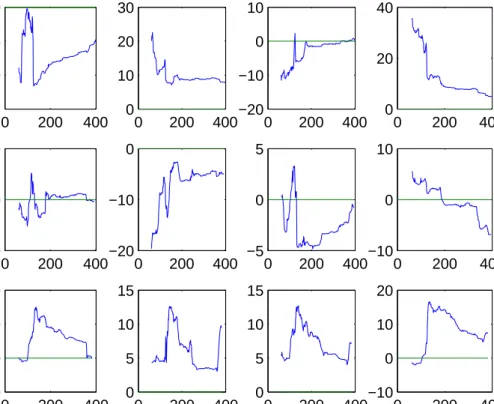
The forecast results of PCovR and PCR are summarized in Table 4 (for single factor models withp= 1) and Table 5 (for multiple factor models withp≤4). The table rows show the four forecasted variables and the three considered forecast horizons, and the columns show the applied forecast method. The MSE’s of PCR and PCovR are measured relative to the MSE of the AR benchmark model. For PCovR, results are shown both for the (data-based, time dependent) CV weightswand for the (a posteriori, time independent) optimal choice of a fixed weight w. This (a posteriori) optimal choice is not feasible in practice, but it serves as a benchmark to evaluate the quality of the CV weights. The last four columns show the forecast gains of PCovR as compared to PCR over the full sample and over three sub-samples, two (70-80 and 81-91) with 132 months and one (92-03) with 144−hmonths wherehis the forecast horizon.
<<Tables 4 and 5 and Figure 1 to be included around here.>>
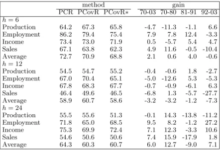
Table 4 shows that the PCR and PCovR single factor models both improve much on the AR benchmark and that PCovR provides better forecasts than PCR in nearly all cases. The results of PCovR with CV weight (column ‘PCovR’) are, as expected, somewhat worse than with a posteriori chosen fixed weight (column ‘PCovR*’), but cross validation works reasonably well. The gains are, on average, largest for production and sales, and smallest for income. Averaged over the four variables and over the full sample period, the MSE gain of PCovR as compared to PCR is 18.6% forh= 6, 23.4% forh= 12, and 26.3% forh= 24. The gain tends to be larger for longer forecast horizon and for early sample periods.
A comparison of Tables 4 and 5 shows that multiple factor models provide better fore-casts than single factor models. Further, PCR improves relatively more than PCovR by adding extra factors. Stated otherwise, the first PCovR factor is a better predictor than the first PCR factor, but additional PCR factors add more to the forecast power than ad-ditional PCovR factors. For a horizon ofh= 6 months, the full sample gains are 7.9% for employment, 4.9% for sales, 0.5% for income and −4.7% for production, with an average
gain of 2.1%. The forecasts are worse forh= 12, with an average loss of 3.2%. The most consistent gains are forh= 24, with an average gain of 6.0%. PCovR does not succeed in forecasting the production series any better than PCR, but forecast gains can be achieved for the other three series. This result means that, with the set-up chosen in Section 5.1, none of the two methods is uniformly better.
Figure 1 shows the MSE gains when evaluated over forecast intervals starting in 1970.01 and ending at varying times, ranging from 1975.01 till the end of the full sample period. The gains are most persistent forh= 24, with largest gains in initial periods and with losses sometimes later on. As concerns the prediction of the production series, forh= 6 PCovR looses much on PCR in initial periods and it relatively improves in later periods, whereas forh= 24 it gains much in initial periods but looses afterwards.
5.3
Further comparison of PCovR and PCR
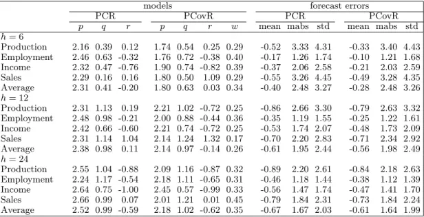
Table 6 summarizes some results on the structure of the selected multiple factor forecast models of PCovR and PCR and on the series of forecast errors of both methods. The rows in this table are the same as in Tables 4 and 5. The first columns of the table show the mean values of the parameters (p, q, r, w) of the selected forecast models. On average, PCovR uses somewhat fewer factors than PCR, whereas the average lagsqandrare comparable for both methods. The cross validation weightwdoes not vary much across the considered variables and forecast horizons and lies mostly between 0.2 and 0.4.
The last columns in Table 6 show three statistics of the forecast errors, that is, the mean value, the mean absolute value, and the standard deviation. PCR and PCovR have roughly the same bias and variance. The bias tends to be somewhat smaller for PCovR, and the variance is smaller for PCR ifh= 12 but it is smaller for PCovR ifh= 24. Both methods have a comparable mean absolute error. This result indicates that outliers do not play an important role, which could be expected because the data in Stock and Watson (2005) have been treated for outliers.
We also performed the test of Diebold and Mariano (1995), with robust standard errors, to examine whether PCovR provides a significantly lower MSE than PCR. For multiple factor models, the differences are not significant when evaluated over the full sample period. However, PCovR is significantly better than PCR for some of the variables over some of the subperiods 1970-1980, 1981-1991 and 1991-2003, six times at a 10% significance level and four times at a 5% level. Further, PCovR is never significantly worse than PCR for any of the series over any of the subperiods or over the full sample period, at a 10% significance level. As could be expected from the results in Table 4, PCovR is often significantly better than PCR for single factor models.
<<Table 6 to be included around here. >>
6
Conclusion
In this paper, we considered the Principal Covariate Regression (PCovR) method. This method estimates factors that approximate the predictorsX and the dependent variabley by minimizing a criterion that consists of a weighted average of the squared errors for y and those forX. We presented an iterative estimation method for the resulting nonlinear estimation problem and discussed the choice of weights in the criterion function. The forecast quality of PCovR under various circumstances was analyzed by means of a simulation study. Further, an empirical comparison of PCovR and PCR was made by one-year-ahead forecasts of four macroeconomic variables (production, income, employment and manufacturing sales). The results show that PCovR can be a valuable tool in forecasting.
We conclude by mentioning some extensions that are of possible interest. In the empirical application, the model structure (p, q, r) was selected by BIC. Another option is to use forecast oriented selection methods, for instance, cross validation methods. Further, we showed that, to prevent overfitting, the PCovR weight should be small if the number of predictors is large. It is of interest to develop methods for regularization of PCovR to prevent overfitting for larger weights. As an alternative, first a subset of the predictors can be selected and then PCovR can be applied (with larger weights) on this smaller set.
References
[1] Bai, J., and S. Ng (2002), Determining the number of factors in approximate factor models, Econometrica70, pp. 191-221.
[2] Borg, I., and P.J.F. Groenen (2005),Modern Multidimensional Scaling, 2-nd ed., New York, Springer.
[3] Boivin, J, and S. Ng (2006), Are more data always better for factor analysis?,Journal
of Econometrics 132, pp. 169-194.
[4] Burman, P, E. Chow and D. Nolan (1994), A cross-validatory method for dependent data,Biometrika 81, pp. 351-358.
[5] De Leeuw, J. (1994), Block relaxation algorithms in statistics, in H.H. Bock, W. Lenski and M.M. Richter (eds.), Information Systems and Data Analysis, Berlin, Springer Verlag, pp. 308-324.
[6] De Jong, S., and H.A.L. Kiers (1992), Principal covariate regression,Chemometrics and
[7] Diebold, F.X., and Mariano, R.S. (1995), ”Comparing Predictive Accuracy,” Journal
of Business and Economic Statistics, 13, 253-263.
[8] Forni, M., M. Hallin, M. Lippi and L. Reichlin (2000), The generalized dynamic factor model: identification and estimation, Review of Economics and Statistics82, pp. 540-554.
[9] Forni, M., M. Hallin, M. Lippi and L. Reichlin (2003), Do financial variables help forecasting inflation and real activity in the euro area?,Journal of Monetary Economics
50, pp. 1243-1255.
[10] Hansen, B.E. (2005), Challenges for econometric model selection,Econometric Theory
21, pp. 60-68.
[11] Heij, C., P.J.F. Groenen and D.J. van Dijk (2005), Forecast comparison of principal component and principal covariate regression, Research Report 2005-28, Econometric Institute Rotterdam. Submitted.
[12] Heij, C., P.J.F. Groenen and D.J. van Dijk (2006), Improved construction of diffusion indexes for macroeconomic forecasting,Research Report 2006-03, Econometric Institute Rotterdam. Submitted.
[13] Heiser, W.J. (1995), Convergent computation by iterative majorization: Theory and applications, in W.J. Krzanowski (ed.), Recent Advances in Descriptive Multivariate
Analysis, Oxford, Oxford University Press, pp. 157-189
[14] Kiers, H.A.L. (2002), Setting up alternating least squares and iterative majorization algorithms for solving various matrix optimization problems,Computational Statistics
and Data Analysis41, pp. 157-170.
[15] Kiers, H.A.L. (1990), Majorization as a tool for optimizing a class of matrix functions,
Psychometrika55, pp. 417-428.
[16] Lange, K., D.R. Hunter and I. Yang (2000), Optimization transfer using surrogate objective functions,Journal of Computational and Graphical Statistics9, pp. 1-20. [17] Pesaran, H, and A. Timmermann (2005), Real-time econometrics,Econometric Theory
21, pp. 212-231.
[18] Phillips, P.C.B. (2005), Automated discovery in econometrics,Econometric Theory21, pp. 3-20.
[19] Racine, J. (2000), Consistent cross-validatory model-selection for dependent data: hv -block cross-validation,Journal of Econometrics99, pp. 39-61.
[20] Stock, J.H., and M.W. Watson (1999), Forecasting inflation,Journal of Monetary
Eco-nomics44, pp. 293-335.
[21] Stock, J.H., and M.W. Watson (2002a), Forecasting using principal components from a large number of predictors, Journal of the American Statistical Association 97, pp. 1167-1179.
[22] Stock, J.H., and M.W. Watson (2002b), Macroeconomic forecasting using diffusion indixes, Journal of Business and Economic Statistics20, pp. 147-162.
[23] Stock, J.H., and M.W. Watson (2005), Implications of dynamic factor models for VAR analysis, Working Paper.
[24] Stock, J.H., and M.W. Watson (in press), Forecasting with many predictors, in G. El-liott, C.W.J. Granger and A. Timmermann (eds.),Handbook of Economic Forecasting, North-Holland, Amsterdam (to appear).