monthly wind speed forecasting in the uk
by
Petros Kritharas
BSc (Hons), MSc
A doctoral thesis submitted in partial fulfilment of the requirements for the award of Doctor of Philosophy of
Loughborough University.
August 2013
author’s written permission.
This thesis was typeset in X E TEX and its format and style were based on the PhD template from the Electrical Engineering Department of The University of Edinburgh, authored by George Taylor.
This is to certify that I am responsible for the work submitted in this thesis, that the original work is my own except as specified in acknowledgements, footnotes or references, and that neither the thesis or the original work contained therein has been submitted to this or any other institution for a degree.
Signature:
Date:
Πέτρος Κριθαρᾶς
Wind is a fluctuating source of energy and, therefore, it can cause several technical impacts. These can be tackled by forecasting wind speed and thus wind power. The introduction of several statistical models in this field of research has brought to light promising results for improving wind speed predictions. However, there is not converging evidence on which is the optimal method. Over the last three decades, significant research has been carried out in the field of short-term forecasting using statistical models though less work focuses on longer timescales.
The first part of this work concentrated on long-term wind speed variability over the UK. Two subsets have been used for assessing the variability of wind speed in the UK on both temporal and spatial coverage over a period representative of the expected lifespan of a wind farm. Two wind indices are presented with a calculated standard deviation of 4% . This value reveals that such changes in the average UK wind power capacity factor is equal to 7%.
A parallel line of the research reported herein aimed to develop a novel statistical forecasting model for generating monthly mean wind speed predictions. It utilised long-term historic wind speed records from surface stations as well as reanalysis data. The methodology employed a SARIMAX model that incorporated monthly autocorrelation of wind speed and seasonality, and also included exogenous inputs. Four different cases were examined, each of which incorporated different independent variables. The results disclosed a strong association between
the independent variables and wind speed showing correlations up to 0.72. Depending on
each case, this relationship occurred from 4− up to 12−month lags. The inter comparison
revealed an improvement in the forecasting accuracy of the proposed model compared to a similar model that did not take into account exogenous variables. This finding demonstrates the indisputable potential of using a SARIMAX for long-term wind speed forecasting.
I would like to thank my supervisor Prof. Simon J. Watson for demonstrating great capacity of probity and academic integrity at all times over the duration of this research. His guidance and continued support have been invaluable.
I must also express my gratitude to the funding bodies of this project; the School of Electronic, Electrical and Systems Engineering (former Department of Electronic and Electrical Engineering) at Loughborough University and the SUPERGEN Wind Energy Technologies Consortium established by the Engineering and Physical Sciences Research Council.
Many thanks to Good Energy Ltd for all the technical information and data contributed to this research.
I also wish to express my sincere thanks to the UK Met Office and the BADC for providing access to the UKCIP gridded dataset and the MIDAS data, respectively. The staff of the Met Office Archive in Exeter should also be acknowledged for providing access to the records related to the meteorological stations used in this research.
Also, I am grateful to the staff and postgraduate students of the Centre for Renewable Energy Systems Technology (CREST) at Loughborough University for creating a stimulating working environment, as well as for their friendship.
Above all, I would like to thankΛέλα, ΓιάννηandΜυρτώfor their unwavering support as well
πράσσοντ’· ἐγὼ δὲ ταῦθ’ἅπαντ’ἠπιστάμην.
ἑκὼν ἑκὼν ἥμαρτον, οὐκ ἀρνήσομαι· θνητοῖς ἀρήγων αὐτὸς ηὑρόμην πόνους.”
I know well. Of my free will, my own free will, I erred, and freely do I here acknowledge it. Freeing mankind myself have durance found.
Προμηθεὺς Δεσμώτης
Αἰσχύλος, 525/524-456/455 Π.Κ.Ε
Prometheus Bound
Declaration of originality . . . iii Abstract . . . iv Acknowledgements . . . v . . . vi Contents . . . vii List of figures . . . x
List of tables . . . xii
Acronyms and abbreviations . . . xiv
Nomenclature and Glossary . . . xvii
Published Work . . . xix
1 Introduction 1 1.1 Global Warming: Facts, Effects, and Remedy . . . 2
1.2 Wind Energy Statistics at a Glance . . . 3
1.3 The British Electricity Market . . . 5
1.4 Wind Power Forecasting . . . 6
1.5 Long-Term Wind Speed/Power Forecasting . . . 7
1.6 Initial Constraints and Hypotheses . . . 8
1.7 Research Objectives and Project Milestones . . . 10
1.8 Contribution to Knowledge . . . 11
1.9 Thesis Outline . . . 12
2 Research Context and Literature Review 13 2.1 Methods and Models . . . 13
2.1.1 Probability Distributions . . . 13
2.1.2 Time Series Forecasting Models . . . 14
2.1.2.1 Regression Analysis . . . 15
2.1.2.2 Box-Jenkins Methodology . . . 16
2.1.2.3 Artificial Neural Networks . . . 21
2.1.3 Other Models Based on AI . . . 25
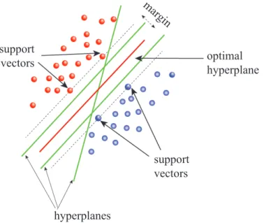
2.1.3.1 Support Vector Machines . . . 25
2.1.3.2 Kalman Filters . . . 28
2.1.3.3 Hybrid Approach . . . 29
2.2 Statistical Models in Long-Term Wind Speed/Power Forecasting: A Literature Review . . . 30
2.3 Chapter Summary . . . 41
3 Data Collection and Analysis 43 3.1 Sources of Data . . . 43
3.1.1 Surface Observations from the UK MIDAS via the BADC . . . 43
3.1.2 ERA-40 Reanalysis Dataset . . . 45
3.3 Factors that may Affect Wind Speed Measurements . . . 51
3.3.1 Site Exposure . . . 51
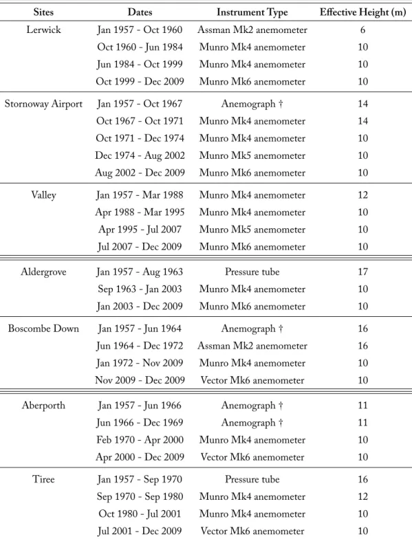
3.3.2 Instrument and Height Measurement Changes . . . 53
3.3.2.1 Vertical Extrapolation and Roughness Length . . . 53
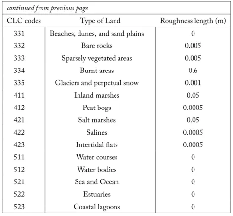
3.3.2.2 CORINE Dataset . . . 59
3.3.3 Data Contamination due to Human Errors . . . 61
3.4 Database . . . 63
3.5 Data Treatment . . . 66
3.5.1 Database Structure . . . 67
3.5.2 Importing the Data . . . 68
3.5.2.1 Ante-process Analysis . . . 70
3.5.2.2 Data Transformation . . . 70
3.5.2.3 Directional Sectors . . . 71
3.5.2.4 Bi-linear Interpolation . . . 74
3.5.3 Data Cleaning Guide . . . 76
3.5.3.1 Icing Events . . . 76
3.5.3.2 Instrument Degradation . . . 77
3.5.3.3 Battery Voltage . . . 77
3.6 Chapter Summary . . . 78
4 Wind Speed Variability Across the UK 79 4.1 Introduction . . . 80
4.2 Background . . . 81
4.2.1 Historic Long-Term Wind Speed Trends . . . 81
4.2.2 Future Projected Trends . . . 82
4.2.3 A Comparison of Wind Indices . . . 84
4.3 Data . . . 85
4.3.1 UKCIP Met. Office Gridded Dataset . . . 86
4.3.2 The Garrad Hassan Wind Index . . . 86
4.4 Calculation of the Different Indices . . . 87
4.5 Results . . . 88
4.5.1 The Annual 29-year and 55-year UK Wind Indices . . . 88
4.5.2 Correlation between Different Wind Indices . . . 92
4.5.3 UK Annual Regional Wind Indices . . . 96
4.6 The Effect of Wind Speed Variability on Wind Energy . . . 96
4.7 Chapter Summary . . . 98
5 Model Development 101 5.1 Data Analysis and Diagnostic Tests . . . 101
5.1.1 Frequency Spectrum . . . 101
5.1.2 Checking for Stationarity . . . 104
5.2 Model Selection and Fitting . . . 106
5.2.1 Persistence Model . . . 106
5.2.2 Seasonal Persistence Model . . . 108
5.2.3 Holt-Winters Model . . . 109
5.2.4 ARIMAX/SARIMAX Models with X-input from MIDAS Dataset . . 109
5.2.5.1 Exogenous Variables . . . 112
5.2.5.2 Model Selection and Fitting . . . 121
5.3 Model Validation and Statistical Errors . . . 124
5.4 Long-Term Wind Predictions at BADC-7 Stations . . . 126
5.5 Practical Implementation of the SARIMAX . . . 131
5.6 Chapter Summary . . . 132
6 Conclusions and Further Direction of Research 134 6.1 Findings . . . 136
6.2 Limitations and Recommendations . . . 139
6.3 Conclusion . . . 141
A Mean Annual Wind Speed per Direction 142 B Instruments and Height Measurement Changes 147 C The BADC Surface Wind Speed Indices 152 D Annual Regional Wind Indices by Season 154 E Augmented Dickey Fuller Test 159 F Correlation Coefficients 163 F.1 Tables for Correlation Coefficients . . . 163
F.2 Tables of Differenced Series for Correlation Coefficients . . . 164
F.3 Tables for Correlation Coefficients between Wind Speed and SST Gradients . 165 G SARIMAX Forecasts for the BADC-7 Stations 167 H SARIMAX Forecasts for the BADC-7 Stations 174 H.1 Stornoway Airport . . . 174 H.2 Valley . . . 174 H.3 Aldergrove . . . 175 H.4 Boscombe Down . . . 175 H.5 Aberporth . . . 175 H.6 Tiree . . . 176 References 177
1.1 The concept of the concentric circle approach . . . 1
1.2 Overview of the processes in BETTA . . . 5
2.1 Illustration of an artificial neural network . . . 21
2.2 Illustration of an SVM classifier based on the margin criterion . . . 26
2.3 Illustration of a higher dimensional feature space for classifying two different sets of data . . . 27
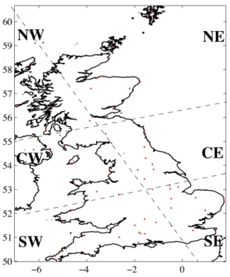
3.1 Regional distribution of stations used in the study . . . 48
3.2 Geographical location of stations used in the study . . . 48
3.3 Wind roses for the BADC-7 sites . . . 52
3.4 Mean annual wind speed by 30◦direction for Stornoway Airport . . . 54
3.5 Mean annual wind speed by 30◦direction for Aldergrove . . . 55
3.6 Mean annual wind speed by 30◦direction for Tiree . . . 56
3.7 Correction in instrumentation’s effective height . . . 58
3.8 Box plot of 55-year index for Lerwick stations . . . 59
3.9 Satellite image for Aberporth station . . . 62
3.10 Monthly and yearly wind speed records at Lerwick station (hard copy) . . . 64
3.11 u′component raw data from ERA-40 . . . 65
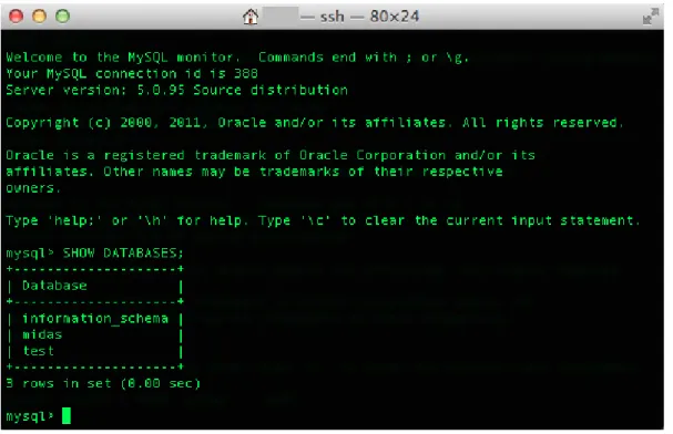
3.12 Using MySQL® databases via the command line client tool . . . 66
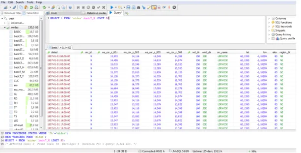
3.13 Using HeidiSQL in order to provide an overview of the databases running within the developed RDBS. . . 67
3.14 Illustration of a bi-linear interpolation . . . 75
4.1 The 29-year and 55-year wind indices with linear trend line fits to each series . . 89
4.2 A comparison between a wind index calculated using the BADC-7 stations and ERA-40 data interpolated to the same sites over the period 1958-2001 . . . 90
4.3 A comparison between a wind index calculated using the BADC-57 stations and ERA-40 data interpolated to the same sites over the period 1958-2001 . . 91
4.4 A comparison between a wind index calculated using the BADC-57 stations and ERA-40 data interpolated to the same sites over the period 1958-2001 . . 91
4.5 A comparison between a wind index calculated using the BADC-57 stations and the GH index over the period 1995-2007 . . . 92
4.6 A comparison between a wind index calculated using the BADC-7 stations and the same index based on CLC classification . . . 93
4.7 A comparison between a wind index calculated using the BADC-57 stations and the same index based on CLC classification . . . 93
4.8 Pearson correlation coefficient calculated using the annual mean wind speeds at the BADC-7 sites as a function of the distance between the different site combinations . . . 95
4.9 UK wind index by region generated using the BADC-57 stations over the period 1983-2011 . . . 97
4.10 Capacity factor of a Vestas V80 2MW turbine as a function of mean wind speed 98
5.1 Wind speed power spectrum, at 10-m height agl for BADC-7 . . . 103
5.2 Seasonal patterns in Case 1 of the BADC-7 stations . . . 105
5.3 Predictions of the 1-month Persistence model at Lerwick . . . 107
5.4 Domain under investigation for correlation between the wind speed over the UK’s grid and several meteorological variables over the remaining grids . . . 115
5.5 Scatter plot matrices between wind speed over the UK and different independent variables for different time lags . . . 116
5.6 Correlation coefficient between wind speed over the UK and wind speed from ERA-40 for a time lag of 12 months . . . 117
5.7 Correlation coefficient between wind speed over the UK and SST form ERA-40 for a time lag of 4 months . . . 118
5.8 Correlation coefficient between wind speed over the UK and MSL form ERA-40 for a time lag of 12 months . . . 118
5.9 Histograms of regular residual for all cases . . . 119
5.10 Domains with the highest correlation between the wind speed over the UK’s grid and the X-inputs . . . 120
5.11 Lags of exogenous variables . . . 121
5.12 Training and testing period of data . . . 122
5.13 Predictions of SARIMAX models over the whole UK . . . 124
5.14 ACF and PACF of the residuals for the SARIMAX over the UK . . . 126
5.15 Predictions of SARIMAX models at Lerwick . . . 129
5.16 Correlograms of residuals at Lerwick . . . 129
5.17 Absolute errors produced by different models at Lerwick . . . 130
A.1 Mean annual wind speed by 30◦direction for Lerwick . . . 143
A.2 Mean annual wind speed by 30◦direction for Boscombe Down . . . 144
A.3 Mean annual wind speed by 30◦direction for Valley . . . 145
A.4 Mean annual wind speed by 30◦direction for Aberporth . . . 146
D.1 Regional winter wind index . . . 155
D.2 Regional spring wind index . . . 156
D.3 Regional summer wind index . . . 157
D.4 Regional autumn wind index . . . 158
G.1 Predictions of SARIMAX models at Stornoway Airport . . . 167
G.2 Correlograms of residuals at Stornoway Airport . . . 168
G.3 Predictions of SARIMAX models at Valley . . . 168
G.4 Correlograms of residuals at Valley . . . 169
G.5 Predictions of SARIMAX models at Aldergrove . . . 169
G.6 Correlograms of residuals at Aldergrove . . . 170
G.7 Predictions of SARIMAX models at Boscombe Down . . . 170
G.8 Correlograms of residuals at Boscombe Down . . . 171
G.9 Predictions of SARIMAX models at Aberporth . . . 171
G.10 Correlograms of residuals at Aberporth . . . 172
G.11 Predictions of SARIMAX models at Tiree . . . 172
3.1 Data Quality Assessment of the BADC-7 . . . 47
3.2 List of of BADC-57 stations . . . 50
3.3 Key to Regions . . . 50
3.4 changes in instrumentation . . . 57
3.5 Value of roughness length based on CORINE land cover classes . . . 61
3.6 Monthly and yearly wind speed records at Lerwick station (digital copy) . . . . 63
3.7 Comparison of storage engines for the MySQL® RDBS . . . 67
3.8 Classification of wind speed direction . . . 72
4.1 Summary of the parameters used in equation (4.1) for calculation of the different indices . . . 88
4.2 Pearson correlation coefficient calculated using concurrent annual values for different indices . . . 94
4.3 Pearson correlation coefficient calculated using annual mean wind speed values for combinations of the BADC-7 stations . . . 95
5.1 ADF test for stationarity . . . 104
5.2 1-month Persistence MSE scores for the BADC-7 stations . . . 107
5.3 1-month and Seasonal Persistence MSE scores for the BADC-7 stations . . . . 108
5.4 ARIMA (0,1,1) MSE scores for the BADC-7 stations . . . 109
5.5 ANOVA for Lerwick station . . . 110
5.6 ARIMAX MSE scores for the BADC-7 stations . . . 111
5.7 SARIMAX MSE scores for the BADC-7 stations . . . 111
5.8 Order of the best SARIMAX for each model . . . 123
5.9 Error of each SARIMAX model . . . 125
5.10 Identifying the order of the best SARIMAX on the training dataset for each model at Lerwick . . . 127
5.11 Order of the best SARIMAX at Lerwick and corresponding statistical errors . . 128
B.1 List of of BADC-57 stations . . . 151
C.1 The BADC Surface Wind Speed Indices . . . 153
F.1 Correlation Coefficients for Actual Wind Speed at the Reference Grid and Wind Speed from the ERA-40 Dataset . . . 163
F.2 Correlation Coefficients for Actual Wind Speed at the Reference Grid and SST from the ERA-40 Dataset . . . 163
F.3 Correlation Coefficients for Actual Wind Speed at the Reference Grid and MSL from the ERA-40 Dataset . . . 164
F.4 Seasonal Differences of Table F.1 . . . 164
F.5 Seasonal Differences of Table F.2 . . . 165
F.7 Correlation Coefficients between Wind Speed at Reference Grid and SST Gradients from the ERA-40 Dataset . . . 166 H.1 Order of the best SARIMAX at Stornoway Airport and corresponding MSE . 174 H.2 Order of the best SARIMAX at Valley and corresponding MSE . . . 174 H.3 Order of the best SARIMAX at Aldergrove and corresponding MSE . . . 175 H.4 Order of the best SARIMAX at Boscombe Down and corresponding MSE . . 175 H.5 Order of the best SARIMAX at Aberporth and corresponding MSE . . . 175 H.6 Order of the best SARIMAX at Tiree and corresponding MSE . . . 176
agl Above Ground Level
ADF Augmented Dickey Fuller test
AIC Akaike’s Information Criterion
ANN Artificial Neural Network
ANOVA Analysis of Variance
AR Autoregressive
ARMA Autoregressive Moving Average model
ARIMA Autoregressive Integrated Moving Average model
ARIMA-ANN Autoregressive Integrated Moving Average - Artificial Neural Network model
ARMAX Autoregressive Moving Average with Exogenous Inputs model
ARX Autoregressive with Exogenous Inputs model
BADC British Atmospheric Data Centre
BETTA British Transmission and Trading Arrangements
BP Backpropagation
CF Capacity Factor
CORINE COoRdinate INformation on the Environment
CLC CORINE Land Cover
CREST Centre for Renewable Energy Systems Technology
DF Dickey Fuller
EEA European Environment Agency
ECWWF European Centre for Medium-range Weather Forecasts
EKF Extended Kalman Filter
ERA-40 ECMWF Reanalysis-40
ERM Empirical Risk Minimisation
EWEA European Wind Energy Association
GM Grey model
GDP Gross Domestic Product
GWEC Global Wind Energy Council
IEA International Energy Agent
KF Kalman Filter
LLS Least Square
LLSSVM Least Square Support Vector Machine
MA Moving Average
MAE Mean Absolute Error
MAPE Mean Absolute Percentage Error
ME Mean Error
MIDAS Met office Integrated Data Archive System
MLP Mutilayer Perceptron
MMU Minimum Mapping Unit
MSE Mean Square Error
MSL Mean Sea Level Pressure
NAO North Atlantic Oscillation
NWP Numerical Weather Prediction
ODBC Open Database Connectivity
PNA Pacific North American
RDBS Relational Database Management System
RMSE Root Mean Square Error
SARIMA Seasonal Autoregressive with Integrated Moving Average
SARIMAX Seasonal Autoregressive Moving Average with Exogenous Input
SE Standard Error
SSE Sum of Squared Errors
SES Simple Exponential Smoothing
SS Simple Seasonal
SST Sea Surface Temperature
SRM Structural Risk Minimisation
SVM Support Vector Machine
◦ A degree of arc
CO2 Carbon dioxide
◦C Degree(s) Celcius
GB Gigabyte is a unit for measuring digital storage equal to one billion Bytes
GW Gigawatt is a unit for measuring electric power equal to one billion Watts or 1,000
megawatts (MW)
ha Hectare is a unit for measuring area equal to 10,000 squared meters (m2)
km Kilometer is a unit for measuring length equal to 1,000 meters (m)
kt Knots is a unit for measuring speed equal to 0.514 ms−1
L Lagging operator
MHz Megahertz is a unit for measuring frequency equal to one million Hertz
MW Megawatt is a unit for measuring electric power equal to one million Watts or 1,000
kilowatts (KW)
MWh Megawatt hour is a unit for measuring electrical energy equal to one million Watt hours
or 1,000 kilowatt hours (kWh)
R2 Coefficient of determination (is a measure of how well the regression line fits the data)
u Wind speed in ms−1
u′ Zonal or eastwards wind component in ms−1
u∗ Friction velocity in the surface layer in ms−1
v′ Meridional or northwards wind component in ms−1
z Height of interest in m
zo Surface roughness length in m
∇ Differencing operator
∇D
Greek Letters
κ von Kármán’s constant (assumed = 0.4)
ρ Correlation coefficient (is a measure of how two variables are linearly related defined as the
covariance of the variables divided by the product of theirσ):ρX,Y= CovσXσX,YX
σ Standard deviation (is a measure of how much dispersed are data from the average value,
defined as the square root of the variance): √σ2
σ2 Variance (is a measure of how data are spread out, defined as the average of the squared
differences from the average or the mean): σ2 =
n
∑
i=1
(xi−X)2
n−1 for the sample andσ
2 = n ∑ i=1 (xi−µ)2 n
for the population
φpLp AR polynomial ofLof orderp
θqLq MA polynomial ofLof orderq
ΦPLP Seasonal AR polynomial ofLPof orderP
ΘQLQ Seasonal MA polynomial ofLQof orderQ
The following papers document the results of this research.
• P. Kritharas and S. J. Watson, ”Long Term Forecasting of Wind Speed Using Historical
Patterns,” in European Wind Energy Conference and Exhibition (EWEC), (Marseille,
France), March 16-19 2009.
• P. Kritharas and S. J. Watson, ”Long term wind speed forecasting based on seasonal
trends,” inProceedings of the ASME3rd Int. Conf. on Energy Sustainability, vol. 2, (San
Francisco, CA, USA), pp. 897-904, July 19-23 2009.
• P. Kritharas and S. J. Watson, ”A comparison of long-term wind speed forecasting
models,”Journal of Solar Energy Engineering, vol. 132, no. 4, p. 041008, 2010.
• P. Kritharas, C. M . Murphy, and S. J . Watson, ”Improved long term wind speed
prognosis using advanced statistical methods,” inEuropean Wind Energy Conference and
Exhibition (EWEC)- Poster session, (Warsaw, Poland), April 20-23 2010.
• S. J. Watson and P. Kritharas, ”Long Term Wind Speed Variability in the UK,” in
European Wind Energy Association Conference (EWEA), (Copenhagen, Denmark), April 16-19 2012.
• S. J. Watson, P. Kritharas, and G. Hodgson, ”Wind Speed Variability across the UK
between 1957 and 2009,”Journal of Wind Energy. Article first published online: 8 OCT
Introduction
T
he following sections act as an introduction to the research topic of this study. By the endof this chapter several answers will have been given so that the readers will be able to appreciate the importance of this particular research. Among others, an example of the answers aimed to be provided is as follows:• Is the use of renewable energy the answer to the damaging effects of global warming? • What is the contribution of wind energy in the overall energy mix and in the economy? • What are the characteristics and constraints of the British Electricity Market that
increasingly necessitate our focus on wind power forecasting?
• What is the importance of wind power forecasting and current research trends? • Why long-term wind speed/power forecasting?
Global Warming Renewables Wind Energy Wind Forecasting Long-term Methods/Models Proposed Model
This endeavour was aided by forming an approach based on identifying the fundamental research boundaries. In a deeper level, the perspective of this study is best described by descending the subject matter. To illustrate this, the concentric circles in Figure (1.1) serve this purpose. The circles represent the different layers each of which deepens in and sets the limits of the different steps taken towards the conduct of this work. The peripheral circle represents the generic research framework where the initial context of global warming is explained. As the circles get closer to the nucleus, a microscopic approach clearly formulates the stages of this work. Firstly, the research context includes the issues that the study is concerned with, the reasons of being important and original, and, how it builds on previous academic work. The problem statement and the research questions then follow progressing to the stage of the methods and approaches considered to be the optimum for addressing the research questions.
1.1 Global Warming: Facts, Effects, and Remedy
The electricity supply risk due to scarcity of conventional energy supplies [1] along with the fear that global warming will preserve its incremental trend [2] are major issues ecumenically recognised. In particular, the uprising trend in global temperature has been addressed long before terms such as global warming and climate change were yet an issue. Hansen et al.
[3] concluded that a rise of about 0.2 ◦C in global temperature between 1960s and 1980s is
associated with anthropogenic carbon dioxide (CO2) emissions. They also predicted that under
the worst case scenario, where no action was taken to cut down the CO2emissions, temperature
would continue to rise. It is of paramount importance to note that at the time that the study was published, the cooling of Northern Hemisphere had led scientists to the common misconception that global temperature declined.
Global warming affects not only ocean rising or polar ice melting but also wind speed. According to a research published, there is an inverse correlation between temperature and wind speed [4].
In the same study, Ren states that an increase of the magnitude of 2 to 4◦C would result in a
weaker atmospheric circulation over the majority of higher latitude regions, which in turn could result in a 4 to 12% decrease in wind speed. There is a need for the public and governments to realise even further this dynamic relationship and the consequences that such an increase in temperature could trigger. Evidence has recently been brought to light that there is a 90%
probability that temperatures will have been risen 3.5 to 7.4◦C by the end of this century [5, 6] due to global warming’s effects. Following the conclusions drawn from the aforementioned
studies, one of the co-authors, Prinn made the following statement: ”there is significantly more
risk than we previously estimated. This increases the urgency for significant policy action.”[7].
The awareness of these issues and their consequences have been evolved into a pragmatic and rational series of actions that need to be taken. Thus, various directives and legislations have been published [8–10]. These policies aim to tackle emissions, reduce the use of fossil fuels, introduce renewables and hence mitigate climate change. The efficacy of these policies is supported by a recent report which manifests that the countries that ratified the 1997 Kyoto Protocol managed to cut down their emissions to about 8% as compared to the levels measured in 1990 [11].
1.2 Wind Energy Statistics at a Glance
Comparing all forms of renewable energy in terms of generation capacity, wind is the one that has been growing at the fastest pace in recent years. Therefore, it has become the flagship of the aforementioned policies. To put some numbers to those facts, Europe by the end of 2012 counted 11.4% of the total energy capacity coming from wind as compared to 2.2% which was recorded in 2000 [12]. This is translated to a five-fold increase of wind power’s share since 2000. Moreover, based on a report published by the Global Wind Energy Council (GWEC), China in 2010, by having installed over 44 GW of wind power capacity, surpassed the 40 GW installed in the US and became the world leader in wind generation [13]. At present, figures are staggering with China counting over 75 GW of installed wind power capacity while the US remain the runner-up with just over 60 GW installed [14]. In the same report, the figures related to future wind generation bring hope and optimism. The projections point out that in the next few years, and in particular by the end of 2017, global wind capacity will stand at about
536 GW as compared to the 197 GW installed at the end of 2010. To mention a fewdomestic
numbers (since the present research is based in the UK), up to December, 2012, 10% of the electricity in Britain was generated from renewables with almost half of it being generated from wind [15].
published by the European Wind Energy Association (EWEA) is worth to be mentioned. According to this study, EWEA has developed an electricity calculator which shows that by
2020 the cost in eper MWh will have been 67, 80, 100, 57 and 74, for gas, coal, nuclear,
onshore wind energy, and offshore wind energy respectively [16]. On top of that, generating electricity from wind is considerably cheaper than photovoltaics by being a more mature technology [17].
It is also very important to mention another report by EWEA where it was found that the contribution to the EU’s Gross Domestic Product (GDP) of wind energy’s industry increased by 33% between 2007 and 2010 [18]. This had an immediate increase in employment by 30% with more than 240,000 jobs being created in times where EU was facing a rate in unemployment of 9.6%. In the very same report, the forecasts about the economic growth that EU will be facing are even more promising. Wind industry will have generated 0.59% by 2020 and almost 1% by 2030 of the EU’s GDP. These figures are translated to an increase of 520,000 and 794,079 in jobs by 2020 and 2030 respectively. On the other side of the Atlantic Ocean, a report published by the US Department of Energy claims that by investing in offshore wind energy only, 200,000 jobs will be supported in the US which in turn can be translated to a $70 billion in annual investments by 2030 [19]. Similarly, the UK’s GDP will be £20 billion higher in 2030 if investment is focussed on offshore wind rather than on gas [20]. In summary, this evidence critically suggests that wind energy not only helps the environment by tackling global warming but also contributes to the economy by creating more jobs.
However, although wind energy is available almost everywhere in the planet, it relies on climatic conditions and also depends on the distinct topography of each place. Therefore, it is considered to be a fluctuating source of energy. For that reason, there are sceptics who believe that wind energy by being intermittent¹ cannot be reliable. In the next sections, the focus will be on the feasibility to predict the output generated from wind and on the various methods/models used to perform this in different time scales. Prior to this, an explanation of the British electricity market will be given in order for the readers to gain a clear understanding of how electricity (including that generated from renewables) is traded.
¹Intermittent and Non-intermittent Generation is defined in Engineering Recommendation P2/6 as follows: Intermittent Generation: Generation plant where the energy source for the prime mover can not be made available on demand. Non-intermittent Generation: Generation plant where the energy source for the prime mover can be made available on demand. [21]
1.3 The British Electricity Market
The wholesale electricity market created for trading electricity within Great Britain, known as the British Transmission and Trading Arrangements (BETTA) [22], obliges generators/suppliers to submit the volume (in half-hourly blocks) of their expected generation/demand to the System Operator (SO) at least an hour ahead of delivery (known as the gate closure time). Therefore, in order for the SO to ensure the delivery of an economic and safe system operation, generators are forced to adhere to their contracts. Wind power has to be traded in the same way as any other form of energy under the BETTA mechanism. However, the variable nature of wind makes the participation to an electricity market such as BETTA more complex. Thus, wind generators have been using several forecasting techniques in order to avoid being penalised for any mismatch between the power contracted to be delivered and that one actually delivered. Figure (1.2) [22] shows on a logarithmic timescale the different processes in BETTA and the actions made by its participants during each stage.
Figure 1.2:Overview of the processes in BETTA
In Great Britain a single trading market consists of the following components [23]:
1. The trade date, which is the date the trade is carried out;
3. The delivery period, which is the length of time that the power is delivered for, which could be between 1 half-hour and an infinite time, for instance an annual contract; 4. The volume, which is the volume chosen to be sold/bought during the delivery period in
MWh. At this point, it is crucial to point out that this volume is fixed and cannot be altered over the course of this specific trade, and finally;
5. The price, which is the cost of the power in £/MWh.
Obviously, generators/suppliers can carry out more than one trade to build up a profiled purchase/sale of power but each trade is constrained as mentioned above.
1.4 Wind Power Forecasting
The value of wind power forecasting has a two-fold importance. Firstly, knowledge of the expected generation output from wind power plants brings confidence to the SOs when trying to achieve reliable and secure operation of the network. Secondly, it enhances the value of wind generated electricity by providing the SOs with vital information when generators/suppliers participate in an energy market such as the market in Great Britain.
This can be achieved both by providing higher value contracts due to better bidding strategies and by minimising imbalance costs. Specifically, in a deregulated market, generators and suppliers (to whom the imbalance risk is often transferred) can avoid being penalised by choosing an optimum bidding strategy. However, this also depends on the market in question. As stated by Bathurst et al. [24], the rules can influence the selection of an appropriate bidding strategy.
So far, most of the research has focused on short-term forecasting of wind conditions. This is mainly due to the operational need for trading electricity a few days or a few hours ahead of gate closure because of the daily fluctuating nature of the demand and the finite response time of generation plants.
Findings vary depending on the selected approach (statistical or physical), the time horizon of the predictions or the area covered (single wind turbine/farm, sub-region, region or country). An
up-to-date comparison and evaluation of the state-of-the-art forecasting systems can be found in a study by Martí et al. [25]. In addition, a series of studies [26–28] provide a comprehensive overview of the prediction models. However, as it will be demonstrated in the next section, SOs, generators, and suppliers have a need of longer term predictions of the power traded so that they can maximise their financial profits and schedule the maintenance of generators and power lines.
1.5 Long-Term Wind Speed/Power Forecasting
A set of motives are germane to long-term wind speed/power forecasting. Initially, long-term predictions of wind energy potential will contribute to the evaluation of the technical feasibility as well as the financial viability of wind projects for their expected operational life span. Such information can be obtained by producing annual wind speed and hence wind power estimates. A recent study reported a 5 to 15% decline of the annual wind speeds measured at 10 m above ground level (agl) across the Northern Hemisphere [29]. However, this work is regarded as being tentative since it takes into account only land surface data for a relatively small period. Nevertheless, the results showed that further work must be carried out looking at the longer timescales. In practice, annual mean wind speeds may vary at a significant rate. As a consequence, long-term variability in wind speeds can lead to misleading assessment of the wind energy yield for both operational and candidate sites. This in turn may result, depending on the specification of the turbines used, in deceptive projections of the payback period of the investment. The latter can prove to be catastrophic for the investors since large fluctuations in the annual mean wind speed may evince that such an investment is uneconomic; hence the project may be classified as non-bankable. This is because setting the terms of concessions and repayment of any loan before granting it is a common practice for bankers and external investors. In the case of wind power projects, they are interested in monthly power predictions in order to evaluate the associated risk and to determine the revenue of the project.
Another motive connected to long-term estimates is that half hourly trading, as it happens in the majority of the liberalised electricity markets (including that of Great Britain), may not be an option for small generators and suppliers due to the overhead of operating a 24-hour trading desk. Some small suppliers of green electricity, including that from wind farms, trade a
month ahead and thus require an indication of the expectedwindinessof the following month. Therefore, any reference for the future state of wind conditions is critical since it would provide suppliers with vital information with regard to the optimum purchasing of base load [30].
Long-term estimates of wind speed/power would contribute to the maintenance schedule for wind farms, the whole operation of which can typically be time-consuming and expensive. Moreover, long-term wind power forecasting would allow SOs to evaluate the potential wind energy production and schedule power systems in a more effective way [31, 32]. Such a perspective would also include the potentiality for SOs to plan and manage the transmission lines.
1.6 Initial Constraints and Hypotheses
Monthly wind speed forecasts were suggested by Good Energy (who supported this research) as such information will integrate into an in-house trading system for purchasing base load months in advance. The purchase of base load has a two-fold importance. Firstly, it reassures SOs that the network will maintain its full capacity. Secondly, it prevents suppliers that generate electricity by renewable sources, such as Good Energy, from being exposed to higher risk during the imbalance settlement process. In case customers have consumed more energy than Good Energy has purchased/generated on their behalf, the company has to buy base load in order to meet the demand. However, this approach may be deemed, under special circumstances, inefficient and expensive. Thus, monthly predictions have been selected to meet the needs of the company.
Moreover, Good Energy has suggested that it may be prudent to use models based on statistical techniques. The reason for their suggestion is based on the fact that running global climate models (GCMs) or regional climate models (RCMs) is not a realistic option for the company’s daily needs. All these models require high specification hardware and are time consuming. Thus, this research considered only models based on statistical techniques.
Two of the major groups of statistical models have been favoured so far in the limited literature of long-term wind speed/power forecasting. The first is the so called autoregressive models and
the second group is inspired by artificial intelligence (AI). Several reasons played a catalytic role in choosing to test the autoregressive models as shown below:
• considerably less need in computational power; • less complexity for the common user;
• access to a vast amount of data that makes it more sensible to use autoregressive models as opposed to AI models that are not dependent on large datasets.
However, as it will be shown in more detail in section 2.2, autoregressive models have not employed so far explanatory variables other than wind speed for generating long-term forecasts. This study aims to test the hypothesis that,
independent meteorological variables are highly correlated with wind speed for different time lags and when they are utilised under a single model that treats wind speed as a dependent variable then the model shows higher accuracy and performance compared to a model which does not.
Prior to presenting a model which, depending on the results, would add value to the daily operations of Good Energy, assessing the variability of wind speed from historic measurements was also deemed prudent. This target was driven solely because wind speed variations can affect the energy yield from wind farms and thus can have an impact on the risk weighed in the return of the investment. Another factor that underpins the assessment of the variability of wind speed derives from a recent survey by DNV KEMA [33] that brought to light evidence that historic wind resource contributes 18% to the total energy production uncertainty. At this point, it should be noted that in 2010 the UK experienced an unprecedented period of particularly low wind speeds which had in turn a huge impact on wind industry [34]. On the contrary, in early 1990s the UK experienced a period of high wind speeds above the usual variation in long-term mean wind speeds [35]. The aim of this line of research is to,
• generate a reliable and cost effective wind index that accounts a considerable long period of historic onshore wind speed data, and
1.7 Research Objectives and Project Milestones
This project has several distinct objectives:
1. to assess the wind speed variability over the UK. 2. to compare the trends with ones from other sources.
3. to convert the changes in wind speed to changes in terms of capacity factor for a typical wind turbine.
4. to investigate the correlation between wind speed and other meteorological variables. 5. to identify a spatial association between the two variables of interest.
6. to take into account different lags in the association between the variables for the development of the model.
7. to compare the proposed model with ones that do not take into account exogenous variables.
8. to introduce an initial framework of model comparison that will contribute to the overall research of long-term wind speed forecasting in the UK.
To accomplish the above objectives the following phases were employed:
• Phase 1: A literature review on the background theory of long-term wind speed forecasting was conducted. This phase included thoroughly any relevant information about past research on the subject. This step also involved the presentation of any relevant theoretical framework. Most importantly, identifying the limitations of the current literature led to conclusions and determined the boundaries of this research. This, as a consequence, shaped the rationale of the research presented herein by highlighting its contribution to the existing body of knowledge.
• Phase 2: Data were collected from onshore historic measurements as well as from other sources such as reanalysis data. During this phase, the raw wind speed records were quality-assessed by identifying and analysing several factors that might affect the
measurements. Several criteria and flagging rules were set to deal with stations that had erroneous, missing or duplicate values. Preventing data contamination due to data entry errors as well as outlier detection were achieved by visually inspecting the time series. Afterwards, the data were stored and maintained thenceforth in a database within the premises of the Centre for Renewable Energy Systems Technology (CREST) for future continuity and other research purposes. This phase resulted in drawing remarks about the limitations, the validity, and the criteria that someone should take into account when dealing with long-term historic onshore measurements.
• Phase 3: Two representative wind indices were created for the UK in terms of both temporal and geographical coverage. This phase employed two groups of data; one consisted of 57 stations covering 29 years of measurements and another one consisted of 7 stations covering 55 years. The calculated standard deviations of these indices were used to estimate the equivalent change in the average UK wind power factor. This phase begot the estimation of the variability of wind speed in the UK and the assessment of how these changes in wind speed translate into changes in wind power. This phase also provided useful insights related to the variability of the wind climate over a period representative of the standard operational life span of a wind project.
• Phase 4: Monthly mean wind speed values were generated. This phase comprised the use of advanced statistical models that consider wind speed as an endogenous input while other variables were used as exogenous inputs. This step resulted in a proposed model that takes into account wind speed over the UK as well as meteorological variables over the Atlantic for different time lags. The high correlation coefficients between wind speed over the UK and the exogenous variables reveal the presence of a strong relationship that, when taken into account, increase the accuracy of monthly mean wind speed forecasts.
1.8 Contribution to Knowledge
The research reported herein is the first known analysis of a UK wind index using surface station observations for a period of greater than 50 years and with an analysis of regional variation. It also presents a contrast between wind indices derived from spatially smoothed datasets, e.g. reanalysis data, and point values from meteorological stations. Moreover, the model proposed for predicting monthly mean wind speeds is the first known autoregressive model that takes
into account exogenous meteorological variables and autocorrelation to generate monthly mean wind speed forecasts.
1.9 Thesis Outline
Chapter 2 defines the research context by discussing the main statistical methods used in time series forecasting and further specifies the direction of this work by presenting a literature review related to the use of these models in long-term wind speed/power forecasting.
Chapter 3 provides information about the source of the data used in this study as well as the necessary actions for eliminating discrepancies and missing or duplicate values.
Chapter 4 presents two long-term wind indices for the UK based on surface stations as well as a UK annual regional wind index.
Chapter 5 presents the proposed statistical model for generating monthly mean wind speed predictions.
The main conclusions are discussed in Chapter 6. The thesis concludes with a series of suggestions for further investigation.
Research Context and Literature Review
M
ost of the work on wind speed/power forecasting has focused on the short-term horizon,thus the majority of the literature published also centres on the short-term predictions. However, there is a justifiable interest in predicting wind speed, and thus wind power, on a monthly, seasonal or even annual basis. This chapter is organised as follows. The first section aims to define the context of this work by presenting the prevalent statistical models used strictly in the field of wind forecasting. The second section contains a comprehensive literature review and discussion narrowing down to the statistical methods/models used in long-term wind speed/power forecasting.2.1 Methods and Models
2.1.1 Probability Distributions
Several studies have dealt with the aspects of wind speed and power statistics. The scope of these studies was to develop appropriate techniques for evaluating the available wind resources. Estimating the availability of wind resources can lead to the evaluation of the performance of current or candidate sites. A way is to determine the probability distribution of wind speed and hence mathematically describe wind’s frequency distribution. So far, different methods have been employed to fit a variety of distributions to wind speed data [36–38] with the Weibull distribution being the most dominant.
The Weibull distribution for wind speed u is expressed by a probability density function.
According to Justus et al. [39], the probability density function is:
where c is the scale factor expressed in wind speed units and k is a dimensionless parameter called the shape factor. Integrating equation (2.1) between zero and a specific value of wind
speed,uxgives its cumulative probability distribution:
P(u≤ux)du=
∫ ux 0
P(u)du= 1−exp[−(ux/c)k] (2.2)
The cumulative probability distribution is used to calculate the probabilityP(u≤ux)whereuis
less thanux. If the shape factorkis equal to 2 then Weibull becomes the Rayleigh distribution
andcis defined as:
c= √2u
π (2.3)
Therefore the Rayleigh distribution is also known as a special case of the Weibull distribution. To summarise, the Weibull is a generalised distribution in which by knowing the scale and the shape factors for a given height it is feasible to adjust these parameters to another desired height [39].
A comprehensive review of the different probability distributions used in wind energy applications along with their mathematical expressions is provided by Carta et al. [40].
2.1.2 Time Series Forecasting Models
A time series is an indexed sample y1,y2, . . . ,yt where the indices 1,2, . . . ,t represent time
spaced at invariant and consecutive intervals. If the data pointsy1,y2, . . . ,yt are assigned to a
random variableYas a finite sequence of values thenYis a discrete variable. If the data points are
assigned as an infinite sequence of values thenYis a continuous variable which has an associated
probability distribution and a probability density function. A sequence of random variables is called stochastic or random process. A deterministic process, as opposed to stochastic, is a process whose future states over time do not involve random phenomena.
accuracy is determined by the difference between the actual value and the forecasted one. This research focuses only on statistical techniques and does not take into account methods based on models of atmospheric physics.
2.1.2.1 Regression Analysis
Regression analysis is a statistical forecasting model which determines the relationship between
a dependent variable and one or more independent variables [41]. Suppose thatYis a dependent
(or endogenous) variable andX is a independent (or exogenous) variable. A regression model
then can be expressed as follows:
Y =α+βX+ϵ (2.4)
where α, βare the coefficients of the dependent variable andϵ stands for the residuals or else
the so called white noise.
The model expressed in equation (2.4) aims to minimise the sum of the squared errors by fitting different values of the variables to the set of observations. The sum of the squared errors (often expressed in the language of statistics as SSE) is expressed as follows:
SSE= n ∑ t=1 (ϵt)2 (2.4)= n ∑ t=1 (yt−(α+βxt))2 (2.5)
The units of the SSE are expressed in ms−1when looking at forecasting errors in wind speed and
in kW when looking at the prediction errors in wind power. Henceforth, this applies accordingly throughout this thesis unless what the SSE is measuring is not explicitly stated.
However, the technique expressed in equation (2.4), also known as regression analysis fit, has a major flaw since the choice of the fitting values is not for the original function. Instead, prior to the selection of the optimum values, the original function is linearised. This justifies the assumption that the variables are not random.
To provide an example, Connor [42] predicted wind speed and direction from equations that individually minimise the least squared errors in wind components. It was then found that the independent variables were highly correlated (intercorrelation) and therefore a forward stepwise regression method was employed. Afterwards, the model was tested against persistence² and climatological models. The analysis showed that the proposed model surpassed both persistence and climatological models in predicting wind speed and direction.
2.1.2.2 Box-Jenkins Methodology
This methodology, firstly presented by Box and Jenkins [43], uses an autoregressive moving average model (ARMA) for forecasting time series by fitting past data of the same series to the model. It is expedient, prior to an explanation of ARMA models, to lay out the rationale underlying the formulation of these models.
A type of a stochastic model which depends on its time-lagged forecasts of the series is named autoregressive (AR) [44]. Essentially, AR is a regressive model. The generalised form of an AR
model of order pis given by Box and Jenkins [43]:
yt =c+φ1yt−1+φ2yt−2+· · ·+φpyt−p+ϵt (2.6)
wherecis a constant,φ1, . . . , φpare the parameters (AR coefficients) of the model,yt−1, . . . ,yt−p
are the time-lagged values of the seriesyt, andϵtis the error term at timetwith mean zero and
constant varianceσ2ϵ. The notationpin ARp indicates the order of the autoregressive process
which is expressed as a polynomial that takes into account only the previous terms of the process
and the error term. Hence, the termorderis the polynomial’s degree or else the highest order
power in the polynomial.
Miranda and Dunn in [45] used a probabilistic approach to develop a model which would treat
wind speed time series as an autoregressive process. The proposed model was an AR of 6th
²A persistence model assumes that the value of a variable for timetwill be the same to the predicted value for timet+lmade at the time origint, wherelrepresents the forward time steps. It is the benchmark model which every other model must compete with in order for the forecasters to assess its performance.
order and when it was compared to the persistence model it showed marginal improvement in its predicting accuracy. When lower order AR models were also tested they proved to be inaccurate. However, the proposed model, despite its simplicity, served as a precursor for other more complex statistical models to follow.
Another type of time series model which regresses against the past errors of the series is also available. This model is called Moving Average (MA) and, similarly to AR, it is a type of
stochastic process. Its generalised form of orderqis given by:
yt =c+ϵt+θ1ϵt−1+θ2ϵt−2+. . .+θqϵt−q (2.7)
where θ1, . . . , θq are the parameters (MA coefficients) of the model, andϵt−1, . . . , ϵt−q are the
time-lagged values of the error. Similar to the AR model, the term orderqrefers to the highest
order power in the polynomial.
LetLoperate onyt, andϵtas thelag operator.
Lkyt =yt−k, ∀k∈ (2.8)
The lag operator shifts the data and the errors either forward (whenk < 0) or backward lags
(whenk>0), and is defined as:
Lyt =yt−1 Lϵt =ϵt−1
L(Lyt) =L2yt =yt−2 L(Lϵt) =L2ϵt =ϵt−2
... ...
Lpyt =yt−p Lqϵt =ϵt−q
(2.9)
Also, let the differencing operator∇be defined as:
∇yt =yt−yt−1 (2.10)
= (1−L)yt (2.11)
With the lagging notation, expressions (2.6) and (2.7) become:
yt=c+ (φ1L+φ2L2+. . .+φpLp)yt+ϵt (2.12)
yt =c+ (1 +θ1L+θ2L
Setting the AR polynomial ofLof orderpas:
Φp(L) = 1−φ1L−φ2L2−. . .−φpLp (2.14)
and the MA polynomial ofLof orderqas:
Θq(L) = 1 +θ1L+θ2L2+. . .+θqLq (2.15)
then, from expressions (2.14) and (2.15), expressions (2.12) and (2.13) become:
Φp(L)yt =c+ϵt (2.16)
and
yt =c+Θq(L)ϵt (2.17)
When these two models are coupled together they produce an ARMA model. This particular combination has been used for forecasting wind speed for short-term horizons [46–48]. In these initial studies, ARMA models were compared against persistence confirming the superiority of the latter only for periods larger than 1 h.
An ARMA model can be employed by simulating hourly averages of wind speeds for different sites, as Balouksis showed [49]. In this particular work, it became apparent that the ARMA model gives good agreement between the simulated and the measured data.
The accuracy of ARMA models for different time periods and different orders(p,q)was assessed
by Milligan et al. in [50]. It was concluded that the best model was of the order of (1, 24). When this model was compared to persistence it showed a 7% and 18% improvement in the first and sixth hour respectively.
An ARMA model with an order(p,q)is written:
yt =c+φ1yt−1+φ2yt−2+. . .+φpyt−p+θ1ϵt−1+θ2ϵt−2+. . .+θqϵt−q+ϵt (2.18)
With the lagging and polynomial notations, expression (2.18) becomes:
A limitation in all the time series models, mentioned so far, is that they require the time series to be stationary³. However, wind speed is not a stationary process and, therefore, another model has been proposed [43]. This is called autoregressive integrated moving average (ARIMA) model. ARIMA outperforms the aforementioned models since it can use non stationary time series by differencing them until stationarity is achieved [43].
Equations (2.6), (2.7) and (2.11) can be combined to give an ARIMA(p,d,q)model:
(1−φ1L−φ2L2− · · · −φpLp) | {z } AR(p) (1−Ld) | {z } I(d) yt = =c+ (1 +θ1L+θ2L2+· · ·+θqLq) | {z } MA(q) ϵt (2.20)
The notationdrefers to the order of the differencing operator∇which is expressed in (2.8). The
order of the differencing operatordrefers to the number of times that the process is transformed.
Each time the differencing operator is applied the transformed series contain one point less data than the original series.
A seasonal autoregressive integrated moving average model (SARIMA), with degreep,q,P,Q,
is an extension of an ARIMA model, which also takes into account seasonality s, and can be
written as a SARIMA(p,d,q)×(P,D,Q)s. These models are ideal when a seasonal behaviour
features the series. Hence the seasonal part may be identical with the non-seasonal one and may well include a seasonal autoregressive term, a seasonal moving average term and a seasonal differencing operator. To distinguish them, the seasonal parts are denoted with capital letters
where P, D, Qare the seasonal AR, the seasonal differencing operator and the seasonal MA
term respectively.
By combining equations (2.6), (2.7), (2.9), and by substituting both AR and MA polynomials
ofLof order p,q,P,Qwe get:
³A stochastic process, whose attributes do not alter over time, is called a strictly stationary process. This means that the variance and the mean of the data do not alter as the process evolves over time.
φp(L)ΦP(Ls)∇d∇sDyt =θq(L)ΘQ(Ls)ϵt (2.21)
where∇D
s is the seasonal differencing operator.
SARIMAX are SARIMA models with exogenous input. The exogenous input X, integrates an ordinary regression model that uses external variables into the SARIMA model. Thus, from
equation (2.17) we get the generic form of a SARIMAX(p,d,q,b)×(P,D,Q)smodel:
φp(L)ΦP(Ls) | {z } AR(p, P) I(d, D) z}|{ ∇d∇D s yt = exogenous input (b) z }| { ηb(L)ξt +|θq (L)Θ{zQ (Ls)ϵt} MA(q,Q) (2.22)
A SARIMAX model discloses a specific weakness which limits its use. This model assumes that the effect the independent variables have on the dependent one occurs at the current time. Thus, it fails to consider effects that take place at different time lags. However, as it will be shown later on in Chapter 5, there are cases that the dependent variable responds to the changes of the exogenous inputs several lags ahead from the time step that the independent variables were changed.
Autoregressive with exogenous variable models have been employed in the past for predicting wind power on the short-term horizon. Such examples include studies like the one published by Durán et al. [51]. In that study the authors developed an autoregressive with exogenous inputs (ARX) model which predicts wind power while it uses information about wind speed as an exogenous input. Wind speed information was retrieved from the European Centre for Medium-range Weather Forecasts (ECMWF). When the proposed model was tested against an AR and a persistence model, it was found that the ARX model outperforms the rest of the models. For a time horizon up to 24 h the exogenous input improves the forecasts on the wind speed up to 14.1% and 26.3% respectively.
Jensen et al. [52] presented the Wind Power Prediction Tool (WPPT). WPPT is also an ARX model which uses the input of Numerical Weather Prediction (NWP) models and wind
speed measurements as exogenous variables. Like most statistical models, WPPT tries to determine the relationship between historical records of predicted wind speed and on-line power measurements. In order to do so, it is based on a self-calibration technique which allows the model to adapt to any changes with respect to time. Forecasts of wind speed and wind direction are produced for wind farms and sub-regions for a time horizon from 0 - 48 h up to 120 h and they are updated 2-4 times per day [53, 54]. WPPT has been operational since 1998 from the Danish transmission system operator (TSO) for predicting the power output from wind farms. The results published by Nielsen and Madsen [55] suggest that WPPT, although it cannot evaluate directly the economical value of the predictions, produces reliable forecasts that, in turn, can be used for load dispatch and day-to-day electricity trade.
2.1.2.3 Artificial Neural Networks
The architecture of artificial neural networks (ANNs) morphologically resembles the human nervous system. Processing is propagated across many units, similar to the way biological neural structures depend on the activity of many neurons.
Input Input layer Hidden layers Output layer Input Input Output
Figure 2.1:Illustration of an artificial neural network
Figure (2.1) illustrates an artificial neural network of multiple inputs, multiple hidden layers
and one single output. The inputs of a neuron, often known assource nodes, are responsible for
receiving the signals from either environmental stimulus or output signals from other neurons. Consequently, the inputs of a neuron are not responsible of any calculation process other than
interceding the signal to the neurons in the hidden layers. The inputs x of an ANN can be
expressed as a vectorx∈. Each neuron has a set of parameters that are being adjusted during
the learning procedure. These parameters are the so called weights and they are associated to
each input of the neuron. Similar to the inputs, the weightswthat are associated to each neuron
can be expressed as a vectorw∈. The neurons in the hidden layer(s) weigh up and adjust each
input by multiplying the received signals with appropriate weights. The associated weighted signals are summed and the cumulative signal is being passed as an argument to an activation function. The result of the function for this argument is the output neuron for the current inputs and for the specified weights, and ends up at other neurons through the output synapses [56].
The output of each neuron can also be expressed as a vectoro∈, and it is defined as:
o= f(w·x) (2.23)
There is a variety of functions used in the activation procedure. Among the most frequent functions used are the linear, the threshold, and the sigmoid functions. Below, the expression for each activation function is given [57]:
• f(x) =x, when the linear function is used,
• f(x) =
10,, ifif xx≥<00,.
, when the threshold function is used, and
• f(x) = 1+1e−ax, when the sigmoid function is used.
There are two distinct characteristics that classify ANNs: their topology and their learning algorithm.
The topology of a network is the layout by which each neuron is connected to other neurons. Different architectures have been proposed with the major groups being the feedforward and recurrent ANNs.
• Feedforward ANNs:
of multiple inputs, hidden layers and outputs. These networks are known as Multilayer Perceptrons (MLPs) whose transmitted signals are passed from the input(s), through the hidden layers, ending up at the output(s). As opposed to the recurrent ANNs that are described below, the reverse flow of the signal is not permitted in feedforward MLPs. The distinct difference between MLPs and single layer Perceptrons is that the neurons in MLPs can use activation functions that single layer Perceptrons cannot. This is due to the inability of Perceptrons to implement differential equations during their optimisation process [58].
• Recurrent ANNs:
To understand the concept of recurrent networks, one would just need to visualise the connections of neurons, shown in Figure (2.1) as arrows forming loops backwards so that they become inputs to either the same neuron or to other neurons. This feed-back connectivity allows recurrent neurons to transmit their signals back and forth until a minimum error is achieved during the learning process. This feature makes recurrent ANNs ideal for use in optimisation, pattern recognition and forecasting problems [58].
Over the evolution of ANNs, several other models have been proposed such as the Hopfield and the Kohonen ones [57]. However, the scope of this section is to embody the essential characteristics and features of models that are described later on in section 2.2 and not to serve as an in-depth literature review of ANNs. Thus, detailed information about these models has been omitted.
The topological structure of ANNs as well as their training algorithm can vary depending on the application that the ANNs will be employed in. The fundamental feature of ANNs is their inherent learning ability through training. During the training of an ANN a learning algorithm is employed so that the ANN could provide users with a solution. The most popular topology used in wind forecasting is the feedforward MLPs based on back propagation (BP) training. In particular, this algorithm falls into the supervised training classification. The neuron during its training minimises the error by employing the method of steepest descent [59]. Initially, the ANN is introduced with an example that describes the problem. Then
the network propagates the signal forward (forward pass) and calculates a potential output
which essentially is a probability based on the values of the given example. The error is afterwards calculated by differencing the output of the ANN and the desired one for the
given example. As a consequence, during the backward pass of the error, the weights of the neurons are adjusted in order to minimise the difference between the output of the ANN and the desired one. This iteration is performed for a cycle of operations until the output of the neuron converges. A comprehensive overview of neural networks, their different architectures and learning algorithms can be found in a study by Haykin [60].
Numerous studies for wind speed and power forecasting have used these models varying the architecture. Beyer et al. [61] presented feed forward ANNs based on BP and radial basis (RBF) to predict 1- and 10-minute means of wind speed. The proposed models added a 10% improvement in accuracy comparing to the Persistence model. However, when the tested networks were trained on a set of low mean wind speeds but tested on a set of high wind speeds they proved to be inferior to Persistence.
Recurrent networks have also been favoured and suggested in several studies that have investigated short-term wind speed/power forecasting, such as the one published by Kariniotakis et al. [62]. In that study advanced ANNs were utilised for predicting the power output of a wind farm for a horizon of 2 hours with a time step of 10 minutes. Two different models were presented where the first one employs wind speed and wind direction while the second model uses information only about wind speed. In the first model the inputs are treated as independent variables in order to generate wind power output forecasts. The second model generates wind speed predictions solely from wind speed measurements on site. Afterwards, these predictions are fed in another model that transforms wind speed into power by using different manufacturers’ wind turbine power curves. When these two models were introduced to a real case it was found that the first model outperforms the second one and the Persistence model.
Both references constitute the first published studies in the field of short-term wind power forecasting. However, over almost 20 years of research, different architectures as well as training algorithms have also been presented. An up-to-date review on the ANNs used in wind speed prediction is available by Sheela and Deepa [63].
To summarise, in contrast to traditional statistical techniques, ANNs adapt changes as the series evolves over time. Adaptation and learning are major characteristics both attained through the training process. Therefore, ANNs have an advantage of being more robust over traditional