Neural Computing for
Event Log Quality Improvement
Hoang Thi Cam Nguyen
Department of Management Engineering
Graduate School of UNIST
Event Log Quality Improvement
Hoang Thi Cam Nguyen
Department of Management Engineering
Event Log Quality Improvement
A thesis
submitted to the Graduate School of UNIST
in partial fulfillment of the
requirements for the degree of
Master of Science
Hoang Thi Cam Nguyen
12/15/2017 of submission
Approved by
_________________________
Advisor
An event log is a vital part used for process mining such as process discovery, conformance checking or enhancement. Like any other data, the initial event logs can be too coarse resulting in severe data mining mistakes. Traditional statistical reconstruction methods work poorly with event logs, because of the complex interrelations among attributes, events and cases. As such, machine learning approaches appear more suitable for reconstructing or repairing event logs. However, there is very limited work on exploiting neural networks to do this task.
This thesis focuses on two issues that may arise in the coarse event logs, incorrect attribute values and missing attribute values. We are interested in exploring the application of different kinds of autoencoders on the task of reconstructing event logs since this architecture suits the problem of unsupervised learning, such as the ones we are considering. When repairing an event log, in fact, one cannot assume that a training set with true labels is available for model training. We also propose the techniques for preprocessing and training the event logs data. In order to provide an insight on how feasible and applicable our work is, we have carried out experiments using real-life datasets.
Regarding the first issue, we train autoencoders under purely unsupervised manner to deal with the problem of anomaly detection without using any prior knowledge of the domain. We focus on developing algorithms that can capture the general pattern and sequence aspect of the data.
In order to solve the second issue, we develop models that should not only learn the representation and underlying true distribution of the data but also be able to generate the realistic and reliable output that has the characteristic of the logs.
List of figures v
List of tables vii
Nomenclature ix
1 Introduction 1
1.1 Problem scenario . . . 1
1.2 Objectives . . . 3
1.3 Outline . . . 4
2 Background and related work 5 2.1 Machine learning background . . . 5
2.1.1 Feed-forward neural networks . . . 5
2.1.2 Recurrent Neural Networks (RNNs) . . . 6
2.1.3 Autoencoders (AEs) . . . 8
2.2 Related work on quality of event logs . . . 13
3 Preliminaries 17 3.1 Event log definition . . . 17
3.2 Datasets . . . 18
3.2.1 Artificial datasets . . . 18
3.2.2 Real-life datasets . . . 19
4 Multivariate anomaly detection 21 4.1 Introduction . . . 21
4.2 Methods . . . 21
4.4 Input data treatment . . . 24
4.5 Experiments . . . 26
4.6 Evaluation criteria . . . 27
4.7 Results . . . 28
4.8 Discussion . . . 33
5 Event log reconstruction 35 5.1 Introduction . . . 35
5.2 Methods . . . 36
5.3 Missing attribute simulation . . . 36
5.4 Input data treatment . . . 38
5.5 Experiments . . . 40
5.6 Evaluation criteria . . . 41
5.7 Results . . . 42
5.8 Discussion . . . 44
6 Conclusion and future work 47 6.1 Conclusion . . . 47
6.2 Future work . . . 48
References 51
Appendix A Statistical Description and Visualization 59
Appendix B Scatter Plot of Anomalous Time 65
Appendix C Receiver Operating Characteristic Curve 69
1.1 The petrinet process model of BPI challenge 2013 dataset . . . 1
1.2 The proposed framework for event log quality improvement . . . 3
2.1 Feed-forward Neural Network . . . 5
2.2 Recurrent Network architecture . . . 6
2.3 A LSTM cell . . . 7
2.4 Autoencoders . . . 8
2.5 The butterfly architecture of undercomplete autoencoder with five layers . . 8
2.6 A standard variational autoencoder . . . 11
2.7 Reparametrization trick . . . 11
2.8 The architecture of a simple sequence autoencoder . . . 12
4.1 Multivariate anomaly detection procedure . . . 22
4.2 Event log pre-processing example . . . 24
4.3 An example of vectorized input . . . 25
4.4 Reconstruction error of Time attribute . . . 29
4.5 Reconstruction error of Activity attribute . . . 30
5.1 Event log reconstruction procedure . . . 36
5.2 Event log pre-processing example . . . 38
B.1 Normal and abnormal of selected activity duration of BPI 2013 log . . . 65
B.2 Normal and abnormal of selected activity duration of BPI 2012 log . . . 66
B.3 Normal and abnormal of selected activity duration of small log . . . 67
B.4 Normal and abnormal of selected activity duration of small log . . . 68
C.1 Receiver Operating Characteristic of Time attribute . . . 70
D.1 Multivariate Anomaly Detection: Directory structure . . . 74 D.2 Event Log Reconstruction: Directory structure . . . 75
1.1 A subset of an event log . . . 2
3.1 Configurations for log generation . . . 19
3.2 A part of a dataset exported by Disco . . . 20
4.1 Choices of hidden size for experiments. . . 27
4.2 Execution Time in multivariate anomaly detection experiments. . . 27
4.3 Performance of Anomalous Time Detector . . . 31
4.4 Performance of Threshold-based Anomalous Activity Detector . . . 32
4.5 Performance of Argmax-based Anomalous Activity Detector . . . 32
5.1 Example of missing attribute value setting . . . 37
5.2 Number of missing values in each dataset . . . 37
5.3 Choices of hidden size for experiments . . . 40
5.4 Execution Time in multivariate anomaly detection experiments. . . 41
5.5 Model performance for missing timestamp value reconstruction . . . 42
5.6 Model performance for missing activity label reconstruction . . . 43
A.1 BPI 2013 Challenge: Descriptive statistics of activity duration and frequency 59 A.2 BPI 2013 Challenge: Descriptive statistics of case duration . . . 59
A.3 BPI 2012 Challenge: Descriptive statistics of activity duration and frequency 60 A.4 BPI 2012 Challenge: Descriptive statistics of case duration . . . 61
A.5 Small log: Descriptive statistics of activity duration and frequency . . . 62
A.6 Small log: Descriptive statistics of case duration . . . 62
A.7 Large log: Descriptive statistics of activity duration and frequency . . . 63
Acronyms / Abbreviations
AE Autoencoder
ELR Event Log Reconstruction
EM Expectation Maximization
fpr false positive rate
KL Kullback-Leibler divergence
LAE Long Short-Term Memory Autoencoder
LSTM Long Short-Term Memory
MAD Multivariate Anomaly Detection
MLP Multi-Layer Perceptron
NN Neural Network
OHC One Hot Encode
RNN Recurrent Neural Network
ROC Receiver Operating Characteristic
tpr true positive rate
Introduction
1.1
Problem scenario
Historical information about execution of business processes can be recorded in so-called
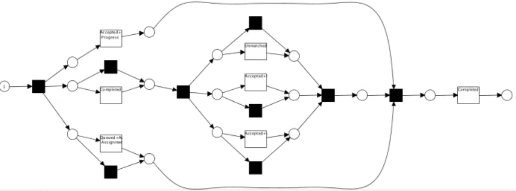
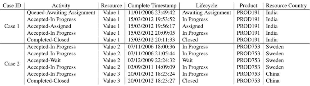
event logsusing data produced by enterprise information systems. A record in an event log is an individual event that occurred in a particular process instance, orcase, and includes attributes such as a case id, timestamp of occurrence, activity label, i.e., what was executed, and resources, i.e., who was in charge of execution/supervision. Event logs enable a plethora of process analyses, such as process discovery, conformance analysis, performance analysis or organisational information mining [51]. For instance, Table 1.1 shows an example event log of a loan origination process and a process model depicted in Figure 1.1 that can be mined from the event log, using traditional process discovery techniques.
Fig. 1.1 A petrinet process model of BPI challenge 2013 dataset mined by using ProM1. This model visualizes the flow of activities between different resources within the company.
Table 1.1 Event log BPI Challenge 2013. Only information of the first two cases is shown.
Case ID Activity Resource Complete Timestamp Lifecycle Product Resource Country
Case 1
Queued-Awaiting Assignment Value 1 11/01/2006 23:49:42 Awaiting Assignment PROD191 India Accepted-In Progress Value 1 15/03/2012 19:53:52 In Progress PROD191 India Accepted-Assigned Value 1 15/03/2012 19:56:17 Assigned PROD191 India Accepted-In Progress Value 1 15/03/2012 20:09:05 In Progress PROD191 India Completed-Closed Value 1 15/03/2012 20:11:33 Closed PROD191 India
Case 2
Accepted-In Progress Value 2 07/11/2006 18:00:36 In Progress PROD753 Sweden Accepted-In Progress Value 2 07/11/2006 21:05:44 In Progress PROD753 Sweden Accepted-Wait Value 2 02/12/2009 22:24:32 Wait PROD753 Sweden Accepted-In Progress Value 2 03/09/2011 14:09:09 In Progress PROD753 Sweden Accepted-In Progress Value 3 20/01/2012 18:23:24 In Progress PROD753 China Completed-Closed Value 3 20/01/2012 18:23:27 Closed PROD753 China
The quality of data-enabled analysis strongly depends on the quality of the underlying data used for it [2]. This holds also for event log-enabled business process analysis. For instance, in the monitoring of process KPIs, low quality information about resources, i.e., inaccurate or incomplete resource attribute values in event logs, prevents calculating an entire class of indicators related with individual resources’ efficiency in executing the tasks to which they assigned.
A certain level of errors in event logs, unfortunately, is often unavoidable, particularly where manual logging is involved. Mans et al. [24], for instance, report that errors in event logs of health care processes mainly occur due to manual logging and that, among them, missing or incorrect case id and resource information occur at higher frequency than missing or abnormal timestamps.
Therefore, more research is needed to address the challenge of improving the quality of event logs, which in turn will enable higher quality analyses of business processes.
Quality of data, in general, can be improved by (i) improving the way in which data are captured while they are being generated and (ii) improving the data after they have been acquired [2]. In this thesis, we focus on (ii), that is, improving the quality of existing event logs. There are two stages to improve the quality of data that have been acquired, namely datacleaningandimputation. The former refers to identifying and removing abnormal values in a dataset, whereas the latter is the process of replacing, or reconstructing, missing values with reliable substituted values.
It should be noted that an event log has unique characteristics which make it different from other types of datasets, such as the ones traditionally used in health care or social science research. While an individual record in other datasets, e.g., medical datasets, can be considered as a complete observation of a phenomenon, an event in an event log is part of a case, which represents an actual observation, that is, a particular execution of a business process. This multi-layered structure of event logs, combined with temporal relations among
events determined by timestamps, require learning models, such as neural networks, able to learn more complex models of data. Due to these characteristics, statistical methods seem to be ineffective, which leaves the problem on how to improve improve the quality of business event log in a more appropriate way. This thesis aims to address this problem.
1.2
Objectives
The goal of this research is to deal with the two aforementioned data quality issues of the event log,anomalous valuesandmissing values, that should be done duringcleaningand
imputationstage. The method proposed in this project usesautoencoders, i.e., a class of deep feed-forward neural networks that aim at reconstructing their own input after having learnt a hidden latent distribution of the input data [14]. The autoencoders developed in this paper are able to handle both continuous, e.g., timestamps, and discrete attributes, e.g., activity and resource labels. Since the three most important attributes carried by all event logs are case id, timestamp and activity, we only use these attributes in our works; and restrict the proposed model on reconstructing the values of timestamp, as an example of numerical attribute, and activity name, as an example of categorical attribute. The remaining attribute, case id, is maintained accurate and complete. We test the performance of different model variants on artificial and real event logs randomly perturbed with noise; then compare them in terms of the efficiency and computation. In addition, we also introduce the way to transform and present an event log into a numeric matrix so that it can be fed into the learning models.
The proposed framework for event log quality improvement is depicted in Figure 1.2. It is important to note that this process can be totally automated without human intervention. There are two procedures corresponding to the main goals in this thesis.
1. The first goal isdata cleaning.
2. The second goal isdata imputation.
Raw event log MultivariateAnomaly Detection
Event Log
Reconstruction Improved event log
1.3
Outline
The remainder of this thesis is organised as follows:
Chapter 2 introduces the background knowledge of machine learning and gives an overview of some topics related to event quality issue.
Chapter 3 provides the preliminaries which are needed for the remainder of this thesis.
Chapter 4 identify the and suggest the approach for detecting anomalies in event logs.
Chapter 5 addresses event log quality issues and provide the solutions on how to repair incomplete event logs.
Background and related work
2.1
Machine learning background
In this section, we would like to give explanations about the definition of the neural networks that we use in our study. This section also addresses some fundamental theoretical aspects for model learning.
2.1.1
Feed-forward neural networks
Input node Hidden node Output node
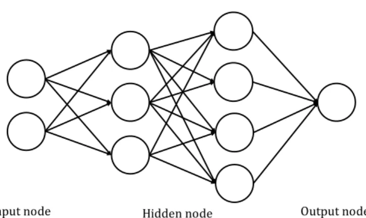
Fig. 2.1 Feed-forward Neural Network
A Feed-forward Neural Network, also called a Multi-Layer Perceptron (MLP), is an artificial neural network of which computational units interconnect in the way that there is no loop or cycle [52]. Thus, in this network, the information can be transferred from input nodes to output nodes through hidden nodes. The network can be comprised of a single layer or multiple layers of perceptron. We can view one perceptron [35] as a mathematical model
that includes a set of weights, and activation functions (linear or non-linear function). These weight values define the behavior of the whole network.
In fact, we can train the network to approximate the values for the weights. Amongst many neural network learning algorithms,backpropagation[38] is the most popular. Back-propagation is an iterative algorithm comprising of two phases,forward phaseandbackward phase. In the former phase, a training set with known output is given. Therefore, we can evaluate the network’s output with the input based on the random weights. After that, in the second phase, we compute the error between the output and the desired output, then take the derivatives of the error with respect to the weight values in the network. Finally, we adjust the weight based on this gradient.
2.1.2
Recurrent Neural Networks (RNNs)
Recurrent Neural Networks
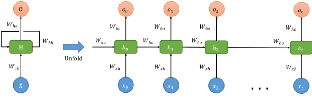
Recurrent Neural Network [36] is a counterpart of MLP, however, the information in the network does not only travel forward. Since there is a loop inside the network that enables information to be persisted, RNNs form a powerful class of models that has an ability to solve multiple prediction and modeling tasks with sequences. The cycle formed by the connections between neurons in RNNs is visualised in Fig. 2.2.
H X O 𝑊𝑥ℎ 𝑊ℎ𝑜 𝑊ℎℎ Unfold ℎ% ℎ& ℎ' 𝑜% 𝑜& 𝑜' 𝑥% 𝑥& 𝑥' 𝑊𝑥ℎ 𝑊𝑥ℎ 𝑊𝑥ℎ 𝑊ℎ𝑜 𝑊ℎ𝑜 𝑊ℎ𝑜 𝑊ℎ𝑜 𝑊ℎ𝑜 𝑊ℎ𝑜
. . .
ℎ( 𝑜( 𝑥( 𝑊𝑥ℎ 𝑊ℎ𝑜 𝑊ℎ𝑜Fig. 2.2 An unrolled architecture of recurrent neural network.
We can see in the diagram that at the timet, one chunk of the network,H, receives input
xtand outputsht. A loop makes it possible to pass information from one time step to the next. If we unfold the RNN diagram above, we can view it as multiple normal neural networks. Each piece passes information to its successor in the network.
More formally, given a sequence of input vectorsx1,x2, ...,xT, each inRn, hidden vectors h1,h2, ...,hT and output vectorso1,o2, ...,oT are computed using the following equations:
ht =f(Wxhxt+Whhht−1+bh)
ot =Whoht+bo
∀t∈1 :T,
(2.1)
whereWxh,Whh,Whoare the input-to-hidden, hidden-to-hidden and hidden-to-output weight matrices, respectively,bhandboare the bias vectors. The undefined hidden vectorh0can be zero or randomly initialised prior to the training procedure. Functionfcan be any activation function.
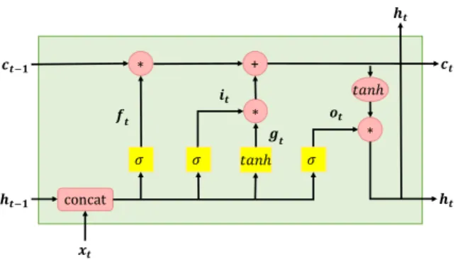
Long Short-Term Memory (LSTM)
𝒉𝒕 𝒄𝒕 𝒉𝒕 ∗ + 𝜎 𝜎 𝑡𝑎𝑛ℎ 𝜎 𝑡𝑎𝑛ℎ ∗ 𝒇𝒕 𝒊𝒕 𝒈𝒕 𝒐𝒕 concat 𝒄𝒕.𝟏 𝒉𝒕.𝟏 𝒙𝒕 ∗
Fig. 2.3 Visualisation of Equation 2.2 for the LSTM module.
Standard RNN lacks the ability to learn long-range temporal patterns due to the vanishing or exploding gradient problems [18, 5]. To alleviate such problems, a modification of the standard RNN with "memory" cells was proposed,long short-term memory(LSTM) [19]. In LSTM, besides hidden and input vectors at each time step, an additional memory cell vector
ct is added. The equations describing the behaviour of LSTM are presented below:
it =σ(Wixt+Uiht−1+bi) ft =σ(Wfxt+Ufht−1+bf) ot =σ(Woxt+Uoht−1+bo) gt=tanh(Wgxt+Ught−1+bg) ct=ft⊙ct−1+it⊙gt ht=ot⊙tanh(ct) ∀t∈1 :T, (2.2)
whereit,ft,ot are referred to as input, forget and output gates; matricesWi,Wf,Wo,Wg
map input vectors to corresponding gate vectors; matricesUi,Uf,Uo,Ugmap hidden vectors to corresponding gate vectors; vectorsbi,bf,bo,bgare the biases,σ is a sigmoid activation
function applied element-wise,⊙ denotes the Hadamard product. The undefined hidden vectorh0and cell vectorc0can be zero or randomly initialised prior to the training procedure.
2.1.3
Autoencoders (AEs)
Autoencoders are a class of neural networks used for unsupervised learning and as generative models [14]. Given a datasetX={xi} ∈Rn, an autoencoder tries to learn a vectorX′having
a distribution similar toX. This is done in two separate processes (see Fig. 2.4 for a standard representation of an autoencoder). First, a vectorZ, i.e., acode, is formed (orencoded) from
X to learn a hidden, orlatentmodelqθ(z|x)of the data, whereθ are the weights and biases
of the encoder; second, a decoder pφ(x|z)reconstructs a vectorX′having similar distribution toX from the codeZ(whereφ are the weights and biases of the decoder neural network).
Z
X X’
f g
Fig. 2.4 An autoencoder comprises of two components: an encoder f and an decoder g, mappings pencoder(h|x)to pdecoder(x|h)
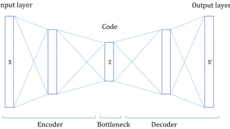
Several hidden layers can be stacked in between input and output layers in both processes, allowing a model to create a higher dimensional representation of the data. The autoencoder of Fig. 2.5, for instance, uses one hidden layer for both encoding and decoding, leading to a 5-layered deep neural network.
X Z X’
Input layer Output layer
Code
Encoder Bottleneck Decoder
Fig. 2.5 The butterfly architecture of undercomplete autoencoder. The dimensions of input and output vectors are the same while the number of neurons of the hidden layers is smaller. The representation of the data lies in the bottleneck which is latent space.
The number of hidden units in the bottleneck layer, i.e., the dimension of the code, can be lower or higher thann. If the size of the code is lower thann, then an autoencoder is forced to learn acompressedrepresentation ofX, by identifying a limited number of interesting features characterising the latent distribution ofX. If the size of the code is higher thann, then an autoencoder can still be used to learn interesting structure in data, particularly if specific constraints on hidden units are enforced, e.g., sparcity of hidden units when processing pixels of an image.
Autoencoders initially have been used for dimensionality reduction and feature learning. The basic idea of autoencoders (with code size lower thann) is similar to the one of Principal Components Analysis (PCA) [1], that is, to project high dimensional data onto a manifold, which can represent data with a lower dimensional code. Unlike PCA, autoencoders are not restricted to linear transformations and they are able to reconstruct their output from latent variables. In addition, it can also obtain the true distribution of the data especially in the task of pattern analysis [4]. Therefore, of more interest to many researchers is the ability of the trained model that can extract useful underlying factors in order to fully understand the data and perform other tasks. Autoencoders have been successfully applied in many real-world problems, such as paraphrase detection [43] or anomaly detection [39]. Nowadays, they also find several applications as generative models, since the learnt codeZcan be used to generate new datasets from the same latent distribution of inputX.
The learning process in an autoencoder aims at optimising a loss functionL(X,X′), where
Lis a suitable likelihood function.Lcan be formulated based on the ultimate objective of the training process. When the data is the output of linear function or the values are in the range of (−∞,∞)(similar to the output in Chapter 4), we can use mean square error which can
be written in Equation 2.3 to measure how close the reconstructed inputx′is to the original inputx.
L(x,x′) = 1
N
∑
i (x′
i−xi)2 (2.3)
When the data resemble a vector of probabilities, i.e., values comprised between 0 and 1, as in the method proposed in Chapter 5, the loss function in Equation 2.4 is used to optimize. This loss function considers the average cross-entropy ofN observationsxiinX.
The cross-entropy between two probability distributions pandqover the same underlying set of observations measures the average number of information units needed to identify an observation drawn from a coding scheme optimised for the distributionqis used, rather than
the true distribution p. L(X,X′) = 1 N N
∑
i=1 xilogx′i+ (1−xi)log(1−xi′) (2.4)In this study, we will look into how to derive the value ofZthrough three models, simple autoencoder, variational autoencoder and sequential autoencoder, in order to construct the event log from the corrupted version of it.
Autoencoder
An autoencoder [37, 23, 7, 17], also called an autoassociator or a Diabolo network, is a special case of feedforward networks, however, it requires less effort during training stage.
Similar to other feedforward neural networks, the neurons in the hidden layers of autoen-coder computes the weighted sums of the input neurons and biases, then passed through a non-linear transformation by some activation function f(.), such as Sigmoid, Tanh or Rectified Linear Unit (ReLU):
z= f(W x+b) (2.5)
Variational Autoencoder (VAE)
Variational Autoencoder [22] is a variant of autoencoder. Similar to autoencoder, the model comprises of encode and decode process which enables extracting the representation of the dataset and mapping the latent variable to the output which distribution is similar to the input. One noticeable difference between two models is how the hidden code is approximated. Vari-ational autoencoder was proposed to perform efficient inference approximation of intractable posterior by using Stochastic Gradient Variational Bayes resulting in fast back-propagation and training process without relying on traditional expensive inference schemes such as Markov Chain Monte Carlo.
Stated more formally, variational autoencoder is trained in such a way that the probability ofX is maximized in the training set according to:
p(x) =
Z
p(x|z,θ)P(z)dz (2.6)
This integral of the marginal likelihood is intractable leading to the intractability of the posteriorp(z|x) =p(x|z)p(z)/p(x), which makes it impossible to apply expectation–maximization (EM) algorithm to approximate. Hence, variational autoencoder deals with this problem by
attempting to optimize thevariational lower bound Lwhich is written as: L(θ,φ,x) =−DKL[qφ(z|x)∥pθ(z)] | {z } KL/regularization term +Eq φ(z|x)[logpθ(x|z)] | {z } reconstruction term (2.7)
whereqφ(z|x)is a probabilistic encoder, the unobserved variableszis a code and pθ(x|z)is a probabilistic decode.
The structure of a standard variational autoencoder is depicted in Fig. 2.6.
X Z
𝜙 𝜃
𝒩
Fig. 2.6 A standard variational autoencoder. Dashed lines denote encoder network approxi-matingqφ(z|x), solid lines denote decoder networkpθ(x|z). The model is jointly learn the parametersφ andθ while training.
The first term in Equation 2.7, Kullback-Liebler (KL) divergence, plays as an additional constraint on how to construct the hidden representation z and it measures how much information is lost when using distribution qto represent distribution p. We need to find
qφ(z|x)so thatDKL[qφ(z|x)∥pθ(z)]is ideally close to zero. To optimizeDKL, we can adopt
gradient descent procedure which uses the gradient of DKL, however, we cannot take the
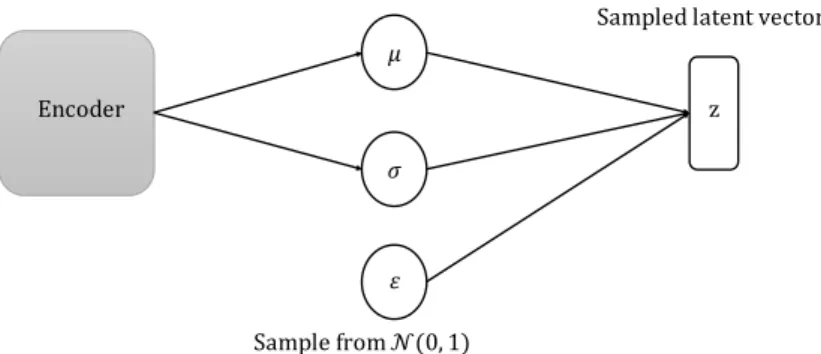
gradient w.r.t φ under the integral sign. This can be solved by usingreparameterization
trick[22] that is depicted in Fig. 2.7.
Encoder 𝜇 𝜎 𝜀 Sample from 𝒩(0, 1) z
Sampled latent vector
The trick suggests that the sample z∼qφ(z|x)can be computed as µ+σ⊙ε where ε∼N(0,1)andqφ(z|x)∼N(z,µ,σ). The term µ andσ are the outputs of encoder layers.
Under this setting, the formula of regularization term at the datapointican be written as:
−DKL[qφ(z)∥pθ(z)] = 1 2 J
∑
j=1 (1+log((σj)2)−(µj)2−(σj)2) (2.8)where µj and σj denote the j-th element of vector µ and σ. The KL divergence can be
computed and differentiated, which allows us to use back-propagation.
The second term of the Lower Bound L is the representation for the performance of generative network (decoder), which measures the error of the outputs and can have either Bernoulli or Gaussian form. Therefore, the loss term can be formulated depends on the training objective as discussed above.
To sum up, a VAE is an autoencoder with added constraints on the encoded representation
Z. In particular, the features in a codeZlearnt by a VAE are forced to roughly follow a given probabilistic distribution p(z), e.g., a unit gaussian distribution. This helps when VAE are used as a generative model, since new output data roughly similar to the input data can be generated by drawing values from such a distribution and pass them into the decoder part of the neural network.
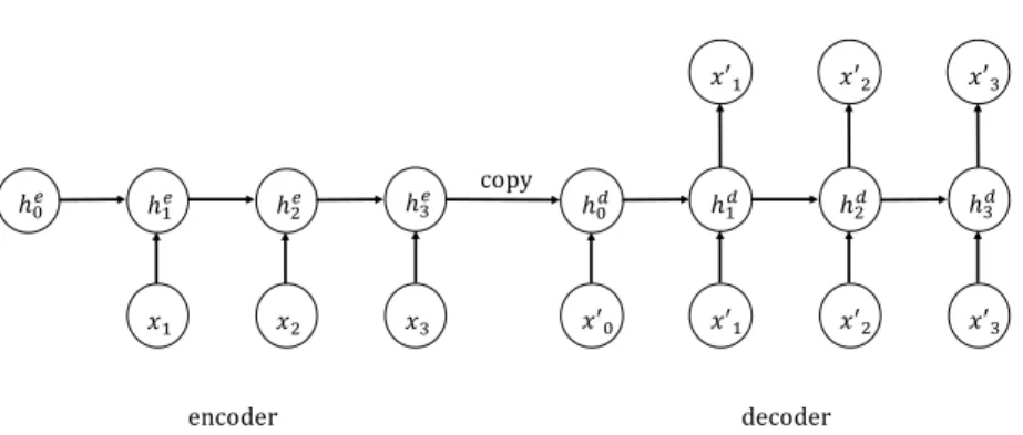
RNN Encoder–Decoder ℎ"# ℎ $# ℎ%# ℎ&# 𝑥$ 𝑥% 𝑥& ℎ"( ℎ $ ( ℎ %( ℎ&( 𝑥′$ 𝑥′% 𝑥′& 𝑥′" 𝑥′$ 𝑥′% 𝑥′& copy encoder decoder
Fig. 2.8 The architecture of a simple sequence autoencoder to reconstruct outputx′ from inputx.
RNN Encoder–Decoder, also known as Sequential Autoencoder, was first proposed by Cho et al. [13] to learn the representation of a sequence of words applied in the field of Natural Language Processing. Similar to AE and VAE, the strategy of this model is to map the input to a fixed-size vector with the encoder, then decode the vector back to the target.
However, with one RNN as a encoder and another RNN as decoder, RNN Encoder–Decoder is able to estimate the conditional probability p(y1, . . . ,yT′)|(x1, . . . ,xT))where(x1, . . . ,xT)
is the input sequence and(y1, . . . ,yT′)is the corresponding output sequence, which can be applied in sequence learning tasks. The illustration of this model is shown in Fig. 2.8.
Different types of recurrent units, such as Long Short-Term Memory unit or Gated Recurrent unit, can be used to build a RNN Encoder–Decoder. Since the work of Tax et al. [47] has shown the empirical results in using LSTM in order to predict the continuation of a running case, in our study, we interested in using LSTM cell block for the encoder and decoder. We call this model Long Short-Term Memory Autoencoder (LAE).
2.2
Related work on quality of event logs
In this section, we review a number of recent works that have proposed in the context of data quality improvement. First, we briefly discuss the data quality issues that were identified, and then we will have a closer look at the previous approaches which were used to encounter these issues.
In Process Mining Manifestor, Aalst et al. [48] define maturity levels ranging from 1 to 5 stars as the indicators of the trustworthiness of an event log used in process mining. Following this, they introduce a guiding principle in the practice of process mining that it should only be applied to well-defined semantic logs which are at least rated as 3-star in order to avoid problematic analysis and unreliable results. Therefore, with high priority, the log should be treated by more systematic approaches.
There has been several works focusing on precisely defining and formulating data quality problem [32, 26, 28]. Different approaches lead to different taxonomies, nevertheless, their findings show that the data problem manifests in very similar ways. Data quality issues in event logs have been classified by Bose et al. [6] and, in the specific context of process mining in the health care, by Mans et al. [24]. Bose et al., in particular, have identified missing, incorrect, imprecise, and irrelevant data as type of sources of event log quality degradation. In addition, they analyze the manner which these issues appear in reality. As the result, the two issues that most frequently occur in real-life logs used in the analysis are missing event, and imprecise activity name; the issue related to timestamp is also a common cause of inconsistent result in process mining. Whereas, Mans et al. point out imprecise resource, i.e. the recorded resource refers to a specific operating room instead of the person who performed the surgery, is more likely to happen than other issues in Hospital Information System (HIS).
The work of Suriadi et al. [46] classifies a set of event log imperfection patterns that may guide the event log quality improvement phase. These patterns help understanding the sources of imperfection in an event log and, therefore, can guide the improvement of logging activities during process execution. This thesis focuses on a closely related, but different issue, that is, reconstructing suspicious and missing values in an event log that has already been acquired. In this thesis, we do not assume any knowledge about the process that has generated an event log.
The quality of event logs is strictly related with detecting noise in event logs, i.e., infrequent behaviour, and with repairing event logs. Noise is typically removed in a pre-processing phase, using frequency-based approaches [11]. As such, it can be seen in our context as a data cleaning activity and the task of detecting noise can be considered as novelty detection. Various state-of-art techniques in novelty detection, such as Frequentist and Bayesian approaches, information theory, and neural network, can be found in [30]. In this paper, the authors categorize all techniques into five groups that are probabilistic, distance-based, reconstruction-based, domain-based, and information-theoretic. Then, they compare the groups in terms of model complexity and application. In the work of Abhinav et al. [44], Hidden Markov Model, which is a typical example of probabilistic approach, has proven to be successfully applied to identify credit transaction fraud. In fact, this method has been extensively used in the context of anomaly detection for time series dataset since it calculates the probability of the behavior happens in the current stage based on the previous stage. In this work, we adopt a similar approach to extract the sequential information from the event log.
Aalst et al. [49] introduce the way to exploitα−algorithm in order to identify anomalous
trace, however, this method requires the complete log containing only normal behaviors to be given as input. In contrast, this thesis assumes that the only information available for repairing and reconstructing values in an event log is the event log itself. In [15], Ghionna et al. proposed a two-step method to filter the exceptional trace by first extracting the normal patterns and then applying a clustering procedure under the assumption that outliers are characterized by infrequent patterns. Recently, Nolle et al. [27] have proposed to use autoencoders for denoising event logs, showing remarkable performance, albeit on artificially generated logs. Event in this case, however, noise in event logs is defined at the event level, e.g., missing or duplicated events, rather than at the event attribute level as we consider in this thesis. Our work also examines the use of reconstruction-based approach, autoencoders, to identify the anomalies. This method relies on frequent data patterns to reconstruct the noisy
input data and use the reconstructed input as a measure of normality, hence, it is susceptible to loops of anomalous data in the logs [27].
Regarding the second context, dataimputation, various methods have been proposed to do this task in large datasets, such as deletion of observations with missing values or reconstructing data using statistical and artificial intelligence techniques. Promising results have been shown particularly in imputation of medical domain datasets [20, 40]. Beaulieu-Jones et al. [20], in the task of dealing data missing completely at random and data missing not at random, find that using bottle-neck architecture autoencoder integrated with dropout as a regularizer gives robust results at a variety of information loss. They also show that autoencoders are able to surpass KNN and SVM even when the missing data is increased. One more advantage of this algorithm is that it runs in linear time. Inspired by this paper, in our work, we use the same approach, but only focus on dealing with data missing completely at random in the logs.
For time series, Zhengping Che et al. [9] deploys a deep neural network based on Gated Recurrent Unit (GRU) [12], which is so-called GRU-D. Their model takes two missing pattern, namely masking and time interval. While the model identifies which inputs are observer or missing based on information from masking, it retrieves input observation pattern from time interval. Both representations, masking and time interval, are fed into the model so that their GRU-D is enabled to not only capture the long-term temporal dependencies of time series but take advantage of the missing patterns to enhance the predictions. They also compare the performance of RNN-based and non-RNN-based to see the benefit of using RNN on extracting sequential information. Since the time attribute in the log can be considered as time series, in this thesis, we also use RNN-based method.
Recently, Gondara et al. [16] propose a multiple-imputation model based on denoising autoencoders, which are able to process a variety of data types (continuous, categorical and mixed), distributions (random and uniform), and missing patterns (missing completely at random and missing not at random). Their model not only perform well on large datasets but also on small size ones. More remarkably, the model is capable to cope well with the situation in which users do not provide complete observations for training. Nevertheless, their model can only takes the fixed length sequence as input, whereas in this thesis, we aim to reconstruct the trace sequence of different length.
In the field of business processes, several ad-hoc methods have been proposed for repairing event logs by reconstructing missing events. Rogge-Solti et al. [34] propose a method based on stochastic Petri nets and Bayesian networks. A similar approach can then be used to improve process documentation [33]. Bayomie et al. [3] have proposed a method
to reconstruct the value of case identifier in an unlabeled event log. These approaches take a different perspective from the one considered in this thesis, since they assume that a process model is available. Missing events or attribute values can be then reconstructed by combining process knowledge with knowledge discovery techniques.
Preliminaries
This section introduces the formal description of the concepts related to event logs. First, we start with the definition of the event log and its notation; then we will discuss on how we collect the datasets for our work.
3.1
Event log definition
An event log is a set of events capturing the instances of a single process. Each process instance is referred to acaseor atraceand each event belonging to a single case is referred to ataskor anactivity. All events corresponding to a trace are chronologically ordered. An event may also carry optional additional information such astime,transaction type,resource,
costs, etc. All these additional properties are considered asattributes. However, in this thesis, we assume the minimal information presented, in which each event has 3 attributes: case id, timestamp and activity name. The first attribute, case id, is complete while other two attributes need to be reproduced to become more reliable.
Before getting into the real-life dataset, let us introduce some required notation of event logs (an example event log is shown in Table 1.1). LetEbe the event universe, i.e. the set of all possible event identifiers. Events are characterised by attributes, e.g., they belong to a particular case, have a timestamp, correspond to an activity, and are executed by a particular person. LetAN={a1, . . . ,an}be a set of all possible attributes names andDai the domain of
attributeai, i.e., the set of all possible values for the attributeai. Attributes can be numerical or categorical. Numerical attributes, e.g., timestamps, assume value within a certain numerical interval, that is, Dai = [vi,min,vi,max]∈R. Categorical attributes assume values within a
Dai =
vi,1, . . . ,vi,K . For any evente∈E and attribute namea∈AN, #a(e)∈Da is the
value of attribute namedafor evente.
Let Did be the set of event identifiers, Dcase the set of case identifiers, Did the set of
activity labels, Dtst the set of possible timestamps, and Dres the set of possible resource
identifiers. For each evente∈E, we define a set of standard attributes: • #id(e)∈Did is the event identifier ofe;
• #case(e)∈Dcaseis the case identifier ofe;
• #tst(e)∈Dtst is the timestamp ofe;
• #act(e)∈Dact is the activity name ofe;
• #res(e)∈Dres is the resource involved ine;
In the pre-processing phase, an event log is transformed into a suitable format to be fed into an autoencoder. The detail on how to do this will be provided in Chapter 4 and 5.
3.2
Datasets
Next, we would like to describe how we collected the datasets. In our experiment, we evaluate the performance of the proposed models by using two real-life event logs collected from an open-source website,4TU1and two artificial event logs generated byPLG2[8]. While deep learning offers great solutions for predictive analytics, it requires sufficient amounts of high dimensional data for more efficient and stable performance [10]. Therefore, in order to get benefit from the deep architecture model and fully extract the valuable information of data, we should choose big-size datasets. In our study, we aim to explore the performance of the models under the extreme situation as well. As the result, for evaluation purposes, we use the process models of different complexities in terms of the number of distinct activities, traces and loops in the logs.
3.2.1
Artificial datasets
We use the PLG2 tool to generate two artificial logs. PLG2 allows to create logs from process models randomly generated. In the thesis, we have considered one small and one large log, characterised by the parameters shown in the Table 3.1:
Table 3.1 Configurations for log generation.. Data Number of traces Number of distinct activities Number of OR gateways Number of AND gateways Small log 2,000 14 0 4 Large log 15,000 10 2 2
The generated log can be saved as BPMN file. We import the BPMN file into Disco2and convert into CSV (Comma Separated Values).
3.2.2
Real-life datasets
From the collection of real datasets, we choose one small dataset, BPI 2013 Challenge [45], and one big dataset, BPI 2012 Challenge [50]. The event logs used in the experiments are briefly described below:
BPI 2013 Challenge: This log comprises 1,487 cases and 6,660 events with 7 different activities obtained from the incident and problem management process of Volvo IT Belgium. The case with the most number of activities comprises of 35 activities. The size of this dataset is relatively small compared to the other dataset.
BPI 2012 Challenge: This log consists of 13,087 cases and 262,200 events capturing the whole process of loan and overdraft application in Dutch Financial Institute. There are 36 different activities observed in the process and the case with the most number of activities comprises of 175 activities. In the experiments with this dataset, the training was done with 5,496 cases while the validation set and the test set consisted of both 1,832 instances.
We use the full version of the datasets in which one activity may occur many times in a trace. The standard format of the dataset file is XES (eXtensible Event Stream). We convert each data into CSV by using Disco. Case ID, complete timestamp and activity are three main information carried by both datasets. Case IDs are anonymized by selecting the anonymization option. An example of dataset which is exported by using Disco is shown in Table 3.2.
More details in terms of the statistical descriptions and visualisations of the datasets are provided in Appendix A.
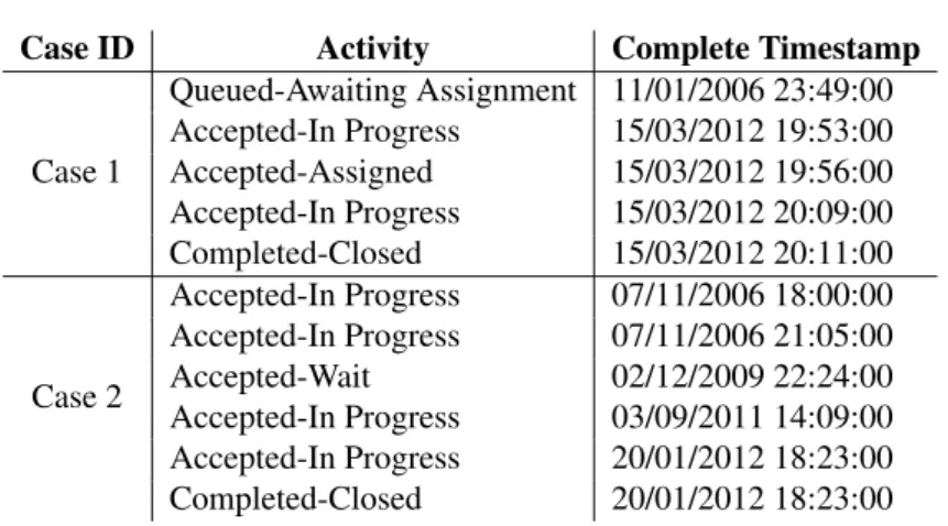
Table 3.2 Event log BPI Challenge 2013.
Case ID Activity Complete Timestamp
Case 1 Queued-Awaiting Assignment 11/01/2006 23:49:00 Accepted-In Progress 15/03/2012 19:53:00 Accepted-Assigned 15/03/2012 19:56:00 Accepted-In Progress 15/03/2012 20:09:00 Completed-Closed 15/03/2012 20:11:00 Case 2 Accepted-In Progress 07/11/2006 18:00:00 Accepted-In Progress 07/11/2006 21:05:00 Accepted-Wait 02/12/2009 22:24:00 Accepted-In Progress 03/09/2011 14:09:00 Accepted-In Progress 20/01/2012 18:23:00 Completed-Closed 20/01/2012 18:23:00
Multivariate anomaly detection
4.1
Introduction
Anomaly detection, also called outlier detection, is a process of identifying unusual patterns in the datasets. Unlike the standard classification task, the anomaly detection problems are mostly addressed by using the concepts in the domain of unsupervised learning, taking only the structure of the dataset into consideration. Detecting the anomalies at an early stage is critical for users since many analysts use extensive amounts of historical data and the analysis is prone to the existence of the anomalies in the dataset. Therefore, there have been various research on anomaly detection system which can be used for many practical applications such as intrusion detection [31], fraud detection [29] and data leakage prevention [42]. However, there is the lack of anomaly detection algorithms as well as available datasets that can used for analyzing the business process containing irregular behaviors due to the fact that anomaly detection is not very frequently researched topic in the field of business process management. Therefore, in this chapter, we present the way to simulate the anomaly and propose a novel anomaly detection algorithm for detecting anomalous events without requiring any domain knowledge. The algorithms work based on the assumption that when there is sufficient or abundant normal data compared to anomalous data, the models are able to generalize the normal behaviors and treat the other data as noise.
4.2
Methods
This section presents in detail the proposed method for detecting anomalous attribute values in event logs. The steps of the proposed are shown in Fig. 4.1. A low quality event log,
i.e., with anomalous values, is taken as input. In a pre-processing phase, event logs are transformed into a format that can be fed into autoencoders. As discussed later in this section, for an autoencoder, each case in an event log represents an observation belonging to the input
X. Hence, each case in an event log is transformed into a matrix of events and features that can be fed into an autoencoder. As far as model training is concerned, in this chapter we experiment with VAE, AE and LAE, which require the same type of input.
Pre-processing Multivariate Anomaly DetectorsAnomaly Detection
Model Training
Event log
(low quality) (Anomaly removed)Event log
Trained Model (VAE, AE, LSTMAE)
Input matrices Output matrices
Fig. 4.1 Multivariate anomaly detection procedure.
After having the autoencoders trained, for each casexwith noise, we can use the model to generate a reconstructed tracex′. We define the reconstruction error indicating the distance between the input vector and the output vector. Under the assumption that the model will reproduce the "normal" values for all attributes, reconstruction error of the normal traces will be smaller than the error of abnormal traces. As the result, we use the reconstruction error as the signal to detect anomalies in the event log. With a choice of threshold, if the reconstruction error is less than the anomaly detection threshold, the variable is normal and vice versa. It turns out that setting the threshold is critical in terms of the performance and the objective of the detector. With a low threshold, we can detect more anomalies, however, there is a trade-off that the number of false positives also increases and vice versa. We report the results by using the average reconstruction error as the threshold. The two detectors for time and activity attributes are set up as follow:
1. Anomalous Time Detector: For detecting anomalous time, the reconstruction error is defined as the absolute value of the difference between the input time and output time attribute. Then, the instance, which the error falls below the threshold, is classified as normal; and the instance is classified as abnormal when the error is exceeded the threshold. Since this detector relies on the choice of threshold, we call it threshold-based detector.
2. Anomalous Activity Detector: In order to detect anomalous activity, we set up two classifiers. One is similar to time anomalous time detector which is the threshold-based detector. However, in this case the error is defined as the mean of the absolute error between probability distribution associated with the output and input activity attribute. In the second detector, instead of using the probability distribution, we use the activity label as the signal of anomaly. The activity is considered as anomalous when its reconstructed label and input label are unmatched. We call this argmax-based detector since the input or output label is the label with maximum probability.
4.3
Anomalous attribute simulation
During the execution of a business process, most of the abnormal instances happened unexpectedly and the structure of these data cannot be observed or described in closed form, which make it impossible to learn the model that can fit the pattern of the anomalies. As a result, it is difficult to simulate a dataset with anomalies given a clean dataset. As far as we are aware, there is no appropriate labeled event log dataset of anomalies available, thus our additional challenge is generating random noisy data points in order to train and evaluate our model.
Initially, we aim to obtain the imbalanced datasets in proportions of 10% anomalies and 90% normal data. These proportions indicate that the likelihood of the anomalies exist in the observation is quite high and this inaccurate information may exacerbates the performance of trained model. However, we want to consider the extreme case in which the ratio of the anomalies is much higher than in reality. The two attributes perturbed are activity and timestamp, so the probability that the mutation occurs is set to 5% in each attribute.
As the anomaly scenario, an activity is anomalous when its label is recored incorrectly. Therefore, we perturb 5% randomly-selected activities by replacing them with another activity which is also randomly sampled.
For the complete timestamp, since we cannot mutate this attribute directly, we make it anomalous indirectly through the duration of the activity corresponding to it. A duration of an activity is anomalous if it is larger than the sum of mean and standard deviation derived from the set of durations of that activity. With this scenario, we replace the duration by anomalous value and repeat until the number of anomalous timestamps is 5% of the total number of data points. After having the anomalous duration, we can transform back to timestamp and derive the cumulative duration within a case. The perturbed duration of selected activities in the four datasets is visualised in Appendix B.
4.4
Input data treatment
Autoencoders require as input observations coded as a matrix of numerical values. Values should also be scaled to facilitate faster convergence. If, in fact, attribute values vary across different ranges, then attributes characterised by larger ranges would be more important than other attributes characterised by smaller ranges during the learning phases. To meet this requirement, an event log is pre-processed as described in the following to transform each case into a matrix of numeric values of fixed size (see Fig. 4.2 for an example).
id case act tst e1 1 A 5 e2 1 B 7 e3 2 B 3 e4 1 C 10 id case CA CB Cc Ctst e1 1 1 0 0 -0.42 e2 1 0 1 0 0.25 e3 2 0 1 0 -1.09 e4 1 0 0 1 1.26 1 0 0 -0.42 0 1 0 0.25 0 0 1 1.26 0 0 0 0 0 0 0 0 0 1 0 -1.09 Case 1 Case 2 e1 e2 e4 e3 Event log Standardisation of attributes “act” (discrete)
and “tst” (continuous) Input of autoencoder
Fig. 4.2 Event log pre-processing for MAD: example
Categorical attributes (see encoding of the activity attribute in Fig. 4.2) are encoded using a one-of-K scheme. That is, for an attributeaia columnci,k in the autoencoder input matrix
is created for each valuevi,k∈Dai. A row is then created for each eventein an event log,
with values in columnsci,k,k=1, . . . ,K assigned as follows:
ci,k(e) = 1 if #ai(e) =vi,k 0 otherwise
As can be seen from the scatter plots shown in Appendix B, the anomalous data points are not far away from the mean in the distribution. In addition, there is a significant difference regarding the duration across different activities, which suggests us to scale the data by using standardisation instead of normalisation; so that the duration with small value will not be shrink. Especially, standardisation will be helpful in case the dataset has some extreme values such as the outliers, it avoids the situation in which the normal value data is scaled to a very small interval. Hence, numerical attributes #ai(e)(see encoding of timestamps Fig. 4.2) are
encoded by standardising their value with the mean valueLmean and standard deviation value
is created such that:
ci(e) =
#ai(e)−Lmean
Lstd , (4.1)
withLmean=#ai(emean),Lstd =#ai(estd)and
emean= 1 N
∑
e ′,∀e′∈E (4.2) estd= r ∑(e′−emean)2 N ,∀e ′∈E (4.3)Obtained rows are then grouped by case id and ordered by timestamp value. As a result, an individual case is represented by a pbyqmatrix, where pis the number of activities in the case andqis the number of columns resulting from the standardisation described above. Since an autoencoder requires a fixed-size matrix as input, zero-padding is applied to all cases for which p<pmax, wherepmaxis the highest number of activities in a case in an event log (see zero-padding of the first two rows for case 2 in Fig. 4.2 in which it is assumed that case 1 is the one with highest number of activities in the event log, another example is shown in Fig. 4.3). In the experiments that we conducted, the results do not depend on the position of the zero-padding rows in an input matrix.
longest length duration OHC activity duration OHC activity
Fig. 4.3 An example of two vectorized inputs of sequence length of 4 and 3. The longest length is five. The white circles denote for zero-padding edges while the blue circles denote for numeric data points.
The objective of the model training step is to train a model that can capture the general behavior of data in an event log. Once a model has been trained, each case in an event log is reconstructed into an output matrix of elementsc′i,jof sizep×q. As a result of the generating step, in the output matrix, the anomalous attributes values are replaced by a new value for numerical attributes and probabilities for the categorical attributes which are supposed to be the real values.
We introduce a masking matrix to indicate zero-padding values which should not be taken into consideration when the model computes the loss for updating weights. Elements
mi,j of the masking matrixM∈Rp×qare defined as:
mi,j= 0 ifci,j=0 (0-padding) 1 otherwise (4.4)
As discussed in Section 4.2, we use distance-based method to classify normal and abnormal behavior, hence, we consider a modified mean squared error loss function, which uses the masking matrix of Eq. 4.4 before averaging across all values in an input matrix:
L(ci,j,c′i,j) = 1 p×q p
∑
i=1 q∑
i=1 mi,j·(ci,j−c′i,j)2 (4.5)4.5
Experiments
A network with many non-linear transformation layers can have the better representation of the data, leading to the fact that in practice people are in favour of deep artificial neural networks than shallow network [25]. However, in all experiments of this thesis, we only use the shallow network to show that our model has real-world applications.
For VAE and AE, we construct a simple architecture with two hidden layers (one in encoder and the other in decoder) and one code layer. The number of neurons in hidden layers is chosen so that it is smaller than the input size. The overview of hidden layer size used for the experiments can be found in Table 4.1. It is important to note here that we can achieve better results compared to the one shown in this thesis if we consider the dimension of all layers as the extra hyperparameters and do fine tuning. We also use non-linear activation function and dropout in the hidden layers, which enables faster convergence and avoids overfitting problem. Based on guidance from the literature [14, 22, 16], internal neurons use Tanhand ReLU activation functions in AE and VAE, respectively. For LAE, we use LSTM cells which hidden size is smaller than the number of features to build the RNN encoder-decoder. The choice of hidden layer used for each dataset is given in Table 4.1.
We conducted several experiments to find good hyperparameters, with early stopping based on the validation loss. Each experiment run in 100 iterations, in each iteration, the data is loaded in batch size of 16. The models are optimised by Adam algorithm [21] withβ1 = 0.9 andβ2= 0.999. We apply adaptive learning rate with an exponential decay factor of 0.99 to adjust the learning rate after each iteration. The weights of each layer are initialized
Table 4.1 Choices of hidden size for experiments.
Data Input size Hidden size
(AE, VAE) Number of features Hidden size (LAE) BPI 2013 280 [100, 50] 8 1 BPI 2012 6,475 [300, 100] 37 20 Small log 210 [100, 50] 15 1 Large log 88 [50, 20] 11 5
from a Xavier normal random distribution. In VAE and AE, we used dropout at 0.2 in order to avoid overfitting problem while in LAE, we use clipping to avoid vanishing/exploding gradient problem.
It is critical to choose the right learning rates since it affect the speed of convergence and the quality of model. Therefore, we tune the learning rate manually. We start the training procedure with the learning rate of 0.01 and gradually decrease by 0.001 after each training. By doing this, we find that the learning rate 0.0001 is sufficient good for the training procedure of three models. We train the model until the condition of early stopping, which the error in the validation set does not improve after 10 epochs, is met; or the maximum number of epochs is reached.
The method has been implemented in Pytorch1. The implementation code is publicly available at2. Experiments run on an Intel i7 Linux machine equipped with 16GB memory and a GeForce GTX 1080 GPU. The execution time of one epoch training is given in Table 4.2.
Table 4.2 Execution time reported in milliseconds.
Data VAE AE LAE
BPI 2013 250 200 300
BPI 2012 1,900 1,500 8,200
Small log 250 200 350
Large log 1,700 1,300 2,000
4.6
Evaluation criteria
Because of the imbalance classes in the dataset, evaluation using the standard accuracy rate is not a good choice since the model may act like general classification models such
1https://github.com/pytorch
that it can cover of the majority examples, whereas the minority ones are misclassified frequently; leading to the high accuracy. The performance of proposed methods should be evaluated mainly based on their ability of identifying the anomalies. Therefore, we assess the performance by determining the metrics of each class label. There are 4 possible outcomes of the binary classification of a variable labeled eitheri- abnormal or j- normal, which are
T Pi(true positive: The labeliis correctly assigned to labeli),FPi(false positive: Label jis incorrectly assigned to labeli),T Ni(true negative: Label jis correctly identified as label j), andFNi(false negative: Label jis incorrectly identified as labeli). The precision/specificity
(πi), recall/sensitivity (ρi) and F-score (fi) of label i are defined as follow:
πi= T Pi T Pi+FPi ρi= T Pi T Pi+FNi fi=2×πi×ρi πi+ρi (4.6)
Then, the average score is the weighted mean of all classes:
π = si×πi+sj×πj si+sj ρ= si×ρi+sj×ρj si+sj f = si× fi+sj×fj si+sj (4.7)
wheresiandsjis the total number of abnormal and normal observations, respectively.
In addition to using the above metrics for evaluation, we also create visualisations for better understanding the performance of the detection models. The first visual evaluation that we use is the histogram of reconstruction errors to examine the distribution of this value across normal and abnormal data. Since we use threshold-based method described in Section 4.2 to separate the usual and unusual data points, we put two overlaid histograms of reconstruction errors of normal and abnormal data in the same plot in order to check whether the detection algorithm can distinguish between them. We also plot receiver operating characteristic (ROC) curve to illustrate two operating characteristics at different threshold settings, please refer to Appendix C for details.
4.7
Results
In this section, we evaluate the computational and the performance of three proposed models. The histograms of reconstruction error of threshold-based anomalous time and anomalous activity detector are presented graphically in Fig. 4.4 and 4.5, respectively. Table 4.3, 4.4 and 4.5 show the evaluation scores for the anomalous time detector, the threshold-based anomalous activity detector and the argmax-based anomalous activity detector in this order.
(a) BPI 2013 - VAE (b) BPI 2013 - AE (c) BPI 2013 - LAE
(d) BPI 2012 - VAE (e) BPI 2012 - AE (f) BPI 2012 - LAE
(g) Small log - VAE (h) Small log - AE (i) Small log - LAE
(j) Large log - VAE (k) Large log - AE (l) Large log - LAE
Fig. 4.4 Reconstruction error of Time attribute. The blue histogram denotes for reconstruction error of normal points and the green one denotes for anomalous points.
(a) BPI 2013 - VAE (b) BPI 2013 - AE (c) BPI 2013 - LAE
(d) BPI 2012 - VAE (e) BPI 2012 - AE (f) BPI 2012 - LAE
(g) Small log - VAE (h) Small log - AE (i) Small log - LAE
(j) Large log - VAE (k) Large log - AE (l) Large log - LAE
Fig. 4.5 Reconstruction error of Activity attribute. The blue histogram denotes for recon-struction error of normal points and the green one denotes for anomalous points.
It is clear that all detectors work better than a random classification model. In particular, VAE and AE are able to discriminate efficiently between normal and anomalous data in the artificial logs. Consider the real-life logs, the models do not yield significant results in BPI 2013 and unfortunately, all models fail in detecting anomaly in BPI 2012. Overall, the anomalous activity detectors show higher performance than the anomalous time detector.
Anomalous Time Detector. The Fig. 4.4g, 4.4h, 4.4j and 4.4k demonstrate that most of the anomalous attributes can be detected effectively by using VAE and AE. In contrast, from Figures 4.4a–4.4f, we can observe the detectors mostly yield nonsensical results for time attribute in two real-life logs. Based on the reconstruction error, the models are unable to distinguish abnormal time from normal ones since the error patterns are similar between two groups. When analyzing the output for the real logs, we find that the detectors encounter several distractions from the normal attribute which has a similar value. The first distraction is the loop in the process flow, which an activity may happen multiple times in a single case. Another distraction is caused by the same range of activity duration. If we take a look insight the duration of normal and abnormal activities visualised in Appendix B, we can recognise that there is no clear borderline between the duration of two groups in two real-life datasets.
Table 4.3 Performance of Anomalous Time Detector.
Data Class VAE AE LAE Support
Precision Recall F-score Precision Recall F-score Precision Recall F-score
BPI 2013 Normal 0.87 0.60 0.71 0.92 0.62 0.74 0.90 0.63 0.74 956 Anomalous 0.07 0.26 0.11 0.15 0.57 0.24 0.12 0.44 0.20 115 Average 0.78 0.56 0.64 0.84 0.62 0.69 0.82 0.61 0.68 1,071 BPI 2012 Normal 0.92 0.64 0.75 0.93 0.70 0.80 0.92 0.67 0.78 43,368 Anomalous 0.12 0.49 0.19 0.14 0.47 0.21 0.12 0.42 0.18 4,455 Average 0.85 0.62 0.7 0.85 0.68 0.74 0.84 0.65 0.72 47,823 Small log Normal 0.98 1.00 0.99 0.98 0.99 0.99 0.94 0.84 0.89 5,086 Anomalous 1.00 0.81 0.89 0.93 0.81 0.86 0.23 0.47 0.31 514 Average 0.98 0.98 0.98 0.98 0.99 0.99 0.88 0.81 0.83 5,600 Large log Normal 0.98 1.00 0.99 0.98 0.99 0.99 0.95 0.69 0.80 21,888 Anomalous 1.00 0.79 0.88 0.89 0.81 0.85 0.16 0.62 0.26 2,112 Average 0.98 0.98 0.98 0.97 0.97 0.97 0.87 0.65 0.72 24,000
Anomalous Activity Detector. Fig. 4.5 gives an insight into the distribution of recon-struction errors of activity variable. Except the figures reported for LAE (Fig. 4.5c, 4.5f, 4.5i and 4.5l), it can be seen that the distribution of the normal and abnormal groups shown in Fig. 4.5 are quite different. For example, in Fig. 4.5a and 4.5b, the distribution of the errors of normal cases is left-skewed while errors of abnormal cases are clustered to the right. More specifically, the majority of normal data has small reconstruction error and the model reproduces the input with large error for most of abnormal data. Nevertheless, the precision is relatively low compared to the recall indicates that the false positive rate is still high. More significant positive results are presented graphically in the artificial logs, which there is no
intersection between the distribution of abnormal and normal data resulting in the ability of the detectors to clearly separate two types of attribute. In conclusion, we achieve sufficient good results in predicting anomalous activity in artificial logs while the performance in real-logs should be improved.
Table 4.4 Performance of Threshold-based Anomalous Activity Detector.
Data Class VAE AE LAE Support
Precision Recall F-score Precision Recall F-score Precision Recall F-score
BPI 2013 Normal 0.99 0.80 0.89 0.97 0.94 0.97 0.97 0.50 0.66 5,015 Anomalous 0.35 0.91 0.51 0.69 0.78 0.73 0.17 0.86 0.28 585 Average 0.95 0.94 0.94 0.95 0.94 0.94 0.89 0.54 0.62 5,600 BPI 2012 Normal 0.97 0.87 0.92 0.96 0.97 0.97 0.93 0.84 0.89 21,552 Anomalous 0.40 0.80 0.53 0.73 0.61 0.67 0.26 0.49 0.34 2,448 Average 0.92 0.86 0.88 0.94 0.93 0.94 0.88 0.66 0.73 24,000 Small log Normal 0.99 1.00 0.99 1.00 1.00 1.00 0.97 0.35 0.52 960 Anomalous 1.00 0.89 0.94 0.97 1.00 0.99 0.14 0.90 0.24 111 Average 0.99 0.99 0.99 1.00 1.00 1.00 0.88 0.41 0.49 1,071 Large log Normal 0.99 1.00 1.00 1.00 1.00 1.00 0.95 0.62 0.76 42,925 Anomalous 1.00 0.95 0.97 0.99 0.96 0.97 0.18 0.73 0.29 4,898 Average 0.99 0.99 0.99 0.99 0.99 0.99 0.87 0.64 0.71 47,823
Table 4.5 Performance of Argmax-based Anomalous Activity Detector.
Data Class VAE AE LAE Support
Precision Recall F-score Precision Recall F-score Precision Recall F-score
BPI 2013 Normal 0.99 0.71 0.83 0.96 0.99 0.97 0.97 0.49 0.65 960 Anomalous 0.27 0.93 0.42 0.84 0.60 0.70 0.16 0.86 0.28 111 Average 0.91 0.74 0.79 0.94 0.95 0.94 0.89 0.53 0.61 1,071 BPI 2012 Normal 0.99 0.36 0.53 1.00 0.85 0.92 0.93 0.87 0.90 42,925 Anomalous 0.15 0.98 0.26 0.43 0.99 0.60 0.29 0.45 0.35 4,898 Average 0.91 0.42 0.5 0.92 0.63 0.7 0.87 0.83 0.84 47,823 Small log Normal 0.99 0.66 0.79 1.00 1.00 1.00 0.94 0.14 0.24 5,015 Anomalous 0.25 0.97 0.40 1.00 0.98 0.99 0.11 0.93 0.20 585 Average 0.92 0.69 0.75 1.00 1.00 1.00 0.86 0.22 0.24 5,600 Large log Normal 1.00 0.79 0.88 0.99 1.00 1.00 0.92 0.75 0.83 21,552 Anomalous 0.35 0.98 0.51 1.00 0.95 0.97 0.17 0.44 0.24 2,448 Average 0.93 0.81 0.84 0.99 0.99 0.99 0.85 0.72 0.77 24,000
Table 4.4 and 4.5 summarises the performance of two different approaches used for the activity classifier, threshold and argmax. During our experiments, we find that there is no absolute superior approach which produces better performance over the other one as long as we are employing the "butterfly" architecture autoencoder. Increasing the size of hidden layers deteriorates the performance of argmax-based detector, whereas the performance of threshold-based detector still remains.
Comparison between the proposed learning models. Comparing the performance between the three models, the results show that VAE and AE outperforms LAE in all datasets, even though we expect that with the complicated computations, LAE will give competitively better results compared to the others. The scores obtained from AE is slightly higher than
those from VAE. In terms of the model complexity, the LAE architecture is more complex than VAE and AE models, resulting in more expensive computational cost (refer to Table 4.2). In addition, tuning LAE requires a lot of effort. From the experiments, we can conclude that AE provides more benefits in this context.
4.8
Discussion
In this work, we investigate the use of autoencoders for detecting anomalies in business process logs and we also integrate our anomaly detection algorithm into real-life datasets. We train the network purely unsupervised by using different types of neural layers, vanilla feed-forward layer and stochastic layer. From the experiments, it is clear that despite the simplicity of the networks and optimisation settings, the autoencoders can be exploit to learn the underlying distribution and general pattern even with the corruption of noise. No prior knowledge about the process is required during model construction stage.
Even though the proposed network has been shown some promising results in solving the problems of anomaly detection, it still faces some challenges and limitations. Firstly, the efficient of the model seems to be restricted by the way we define the boundary between anomalous and normal observations, especially in the case of real logs. When we look at the generated anomalous durations, there are many anomalous data that lies close to the normal, which makes the model hard to distinguish between them. In fact, when we consider the problem arising with the timestamp, we are more interested in fixing imprecise timestamp, i.e. the time does not reflect the true duration of the corresponding activity, than incorrect timestamp, i.e. time is not recorded in order, since it is easy to recognise the later situation. Unfortunately, this pattern is not easily simulated.
Since the model is highly sensitive to the variance introduced by noise, we can improve the performance of current model by identifying and removing easy-to-recognize anomalies before constructing the normal subspace since these anomalies may contaminate the subspace during learning stage.
Another limitation is that the evaluation used for detection algorithm is solely based on metrics and visualisations, which makes it not clear to see how effective our approach is compared to others. In order to give more convinced results, we should compare the performance of our model with other ones.
For the future investigations, we want to cope with the two limitations mentioned above. With the high priority, the lack of standard and appropriate dataset should be solved first in
order to improve the reliability and validity of our models. Then, the next step is to compare our approach with other currently-used frameworks.