High-dimensional change point detection for mean and location parameters

(1)

c

(2)

HIGH-DIMENSIONAL CHANGE POINT DETECTION

FOR MEAN AND LOCATION PARAMETERS

BY

MENGJIA YU

DISSERTATION

Submitted in partial fulfillment of the requirements

for the degree of Doctor of Philosophy in Statistics

in the Graduate College of the

University of Illinois at Urbana-Champaign, 2020

Urbana, Illinois

Doctoral Committee:

Associate Professor Xiaohui Chen, Chair and Director of Research

Professor Annie Qu, University of California, Irvine

Professor Xiaofeng Shao

Professor Douglas G. Simpson

(3)

Abstract

Change point inference refers to detection of structural breaks of a sequence observation, which may have one or more distributional shifts subject to models such as mean or covariance changes. In this dissertation, we consider the offline multiple change point problem that the sample size is fixed in advance or after observation. In particular, we concentrate on high-dimensional setup where the dimension pcan be much larger than the sample sizenand traditional distribution assumptions can easily fail. The goal is to employ non-parametric approaches to identify change points without involving intermediate estimation to cross-sectional dependence.

In the first part, we consider cumulative sum (CUSUM) statistics that are widely used in the change point inference and identification. We study two problems for high-dimensional mean vectors based on the

`∞-norm of the CUSUM statistics. For the problem of testing for the existence of a change point in an independent sample generated from the mean-shift model, we introduce a Gaussian multiplier bootstrap to calibrate critical values of the CUSUM test statistics in high dimensions. The proposed bootstrap CUSUM test is fully data-dependent and it has strong theoretical guarantees under arbitrary dependence structures and mild moment conditions. Specifically, we show that with a boundary removal parameter the bootstrap CUSUM test enjoys the uniform validity in size under the null and it achieves the minimax separation rate under the sparse alternatives when pn. Once a change point is detected, we estimate the change point location by maximizing the`∞-norm of the generalized CUSUM statistics at two different weighting scales. The first estimator is based on the covariance stationary CUSUM statistics, and we prove its consistency in estimating the location at the nearly parametric rate n−1/2 _{for sub-exponential observations. The second} estimator is based on non-stationary CUSUM statistics, assigning less weights on the boundary data points. In the latter case, we show that it achieves the nearly best possible rate of convergence on the order n−1_. In both cases, dimension impacts the rate of convergence only through the logarithm factors, and therefore consistency of the CUSUM location estimators is possible whenpis much larger thann. In the presence of multiple change points, we propose a principled bootstrap-assisted binary segmentation (BABS) algorithm to dynamically adjust the change point detection rule and recursively estimate their locations. We derive

(4)

its rate of convergence under suitable signal separation and strength conditions. The results derived are non-asymptotic and we provide extensive simulation studies to assess the finite sample performance. The empirical evidence shows an encouraging agreement with our theoretical results.

In the second part, we analyze the problem of change point detection for high-dimensional distributions in a location family. We propose a robust, tuning-free (i.e., fully data-dependent), and easy-to-implement change point test formulated in the multivariateU-statistics framework with anti-symmetric and nonlinear kernels. It achieves the robust purpose in a non-parametric setting when CUSUM statistics are sensitive to outliers and heavy-tailed distributions. Specifically, the within-sample noise is canceled out by anti-symmetry of the kernel, while the signal distortion under certain nonlinear kernels can be controlled such that the between-sample change point signal is magnitude preserving. A (half) jackknife multiplier bootstrap (JMB) tailored to the change point detection setting is proposed to calibrate the distribution of our `∞ -norm aggregated test statistic. Subject to mild moment conditions on kernels, we derive the uniform rates of convergence for the JMB to approximate the sampling distribution of the test statistic, and analyze its size and power properties. Extensions to multiple change point testing and estimation are discussed with illustration from numeric studies.

(5)

(6)

Acknowledgments

First and foremost, I owe my heartiest appreciation and immeasurable admiration to my advisor, Professor Xiaohui Chen, for providing invaluable guidance throughout my research. His immense knowledge, broad vision and continual inspiration conveyed the spirit of sincerity in regard to research and helped me to transform scientific arguments into structured association. He granted me with generous time and enlight-ened discussion to address my confusion whenever I needed. I am ineffably indebted to his conscientious patience and encouragement to accomplish my PhD study. I consider it a privilege to have worked under his supervision that pushed me farther than I thought I could go.

I humbly extend my utmost sense of reverence and gratitude to the rest of my committee members: Pro-fessor Annie Qu, ProPro-fessor Xiaofeng Shao and ProPro-fessor Douglas Simpson, for their constructive comments on this dissertation project and consistent advice during my pursuit of doctoral degree. It was a pleasure to benefit from their collective insights and to make acquaintance with their remarkable personalities. I am rewarded from each of my committee members with their erudition and diligence lifelong.

In addition, I am deeply thankful to my husband Dawei Ding for his unconditional love and endless support in my doctoral study. Without his dedication and consolation, my achievement would never be possible. I am also grateful to our families who always expressed confidence and encouragement to us with no hesitation.

The last but not least gratitude goes to all of the Department of Statistics who directly or indirectly helped me over the last five years. The faculty, staff members and colleagues manifested that we formed a whole greater than the sum of its parts. They kept me going when I was frustrated in work and life. I will always remember their warm and motivating words and treasure the strength they passed to me to fight difficulties in the future.

(7)

List of Tables

2.1 Uniform error-in-size sup_α_∈_[0_,_1]|_Rˆ₍_α₎₋_α_| _under _H₀ _{compared with benchmarks. Scenarios}

I-III areV =I,V = 0.8J+ 0.2I andVij= 0.8|i−j|, respectively. . . 29

2.2 Rˆ(0.05): empirical Type I error with nominal level 0.05 for our test. . . 30

2.3 Uniform error-in-size sup_α_∈_[0_,_1]|Rˆ(α)−α|underH0compared with [65] (BnandBnenhanced) and [43] (ψ andψ improved). Tn stands for our test and the values are copied from the last row of Table 2.1. . . 31

2.4 Rˆ(0.05): empirical Type I error with nominal level 0.05 for [65] (Bn andBn enhanced), [43] (ψandψimproved), and ours. Tn stands for our test and the values are copied from the last row of Table 2.2. . . 31

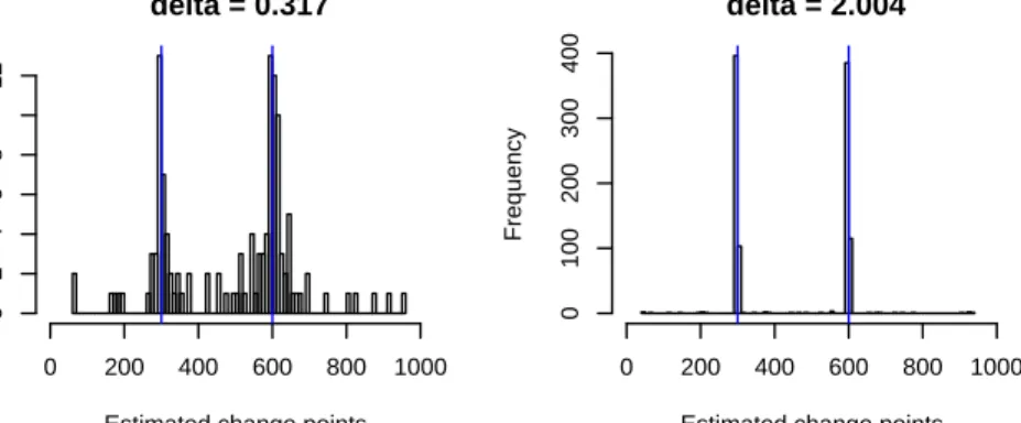
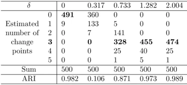
2.5 Multiple change point setup with 2 change points (m1, m2) = (300,600): counts of estimated ˆ ν and ARI. . . 36

2.6 Multiple change point setup with 3 change points (m1, m2, m3) = (300,600,800): counts of estimated ˆν and ARI. . . 37

2.7 Comparison of multiple change points detectors. . . 38

2.8 Quantiles of bootstrapped statistics. . . 42

2.9 Power report of our method for sparse alternative where α = 0.05, tm = 5/10,3/10,1/10. Here,n= 500, p= 600 and the boundary removal is 40. . . 79

2.10 Power report ofBn in [65] for sparse alternative whereα= 0.05,tm= 5/10,3/10,1/10. Here, n= 500, p= 600 and the boundary removal is 40. . . 80

2.11 Power report of ψ in [43] for both sparse and dense Gaussian alternative where α = 0.05, tm= 5/10,3/10,1/10 and spatial dependence structure (I). Here, n= 500, p= 600. . . 80

2.12 RMSE of our estimators ˆm0 and ˆm1/2. Both truncated and non-truncated versions are im-plemented undertm= 5/10 andtm= 1/10. . . 81

2.13 RMSE of estimator in [99]. . . 82

2.14 RMSE of estimator in [37]. . . 82

3.1 Uniform error-in-size underH0. . . 100

3.2 Error-in-size supα|Rˆ(α)−α|forα∈(0,1) andα∈(0,0.1]. . . 100

3.3 Powers for our method using linear and sign kernels, [106, BABS], [65, Jirak], [37, SBS] and [99,Inspect]. . . 102

3.4 Powers under multiple change point scenario using linear kernel. Here, (m1, m2) = (300,600). 103 3.5 Estimation of multiple change points for M = 100. Here, the data is Gaussian distributed with dependence structure (III) andlinear kernel is used. . . 103

3.6 Estimation of multiple change points forM = 100. Here, the data is Cauchy distributed with dependence structure (III) andsign kernel is used. . . 104

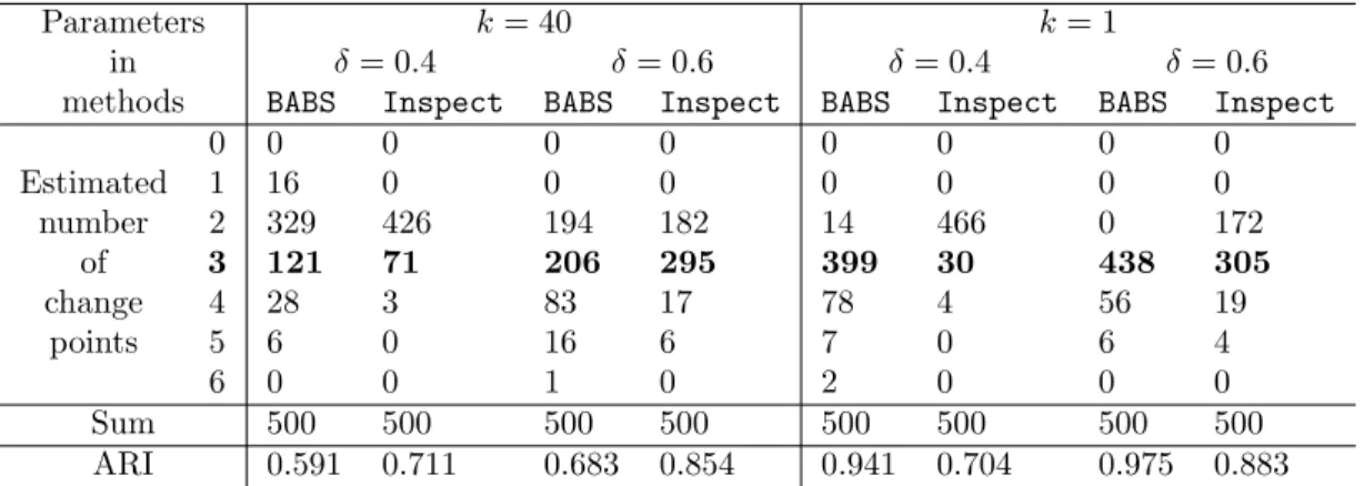
3.7 Estimation of multiple change points forM = 1. Here, the data is Gaussian distributed with dependence structure (III) andlinear kernel is used. . . 105

3.8 Identified change point locations (loci numbers on genome) inACGH dataset. . . 107

3.9 Powers report of our method usinglinearkernel. Here,n= 500, p= 600, α= 0.05 and change point locations aretm=m/n= 5/10,3/10,1/10. . . 127

(10)

3.10 Powers report of our method usingsign kernel. Here,n= 500, p= 600, α= 0.05 and change point locations aretm=m/n= 5/10,3/10,1/10. . . 127

(11)

List of Figures

2.1 Selected setups for comparing ˆR(α) withα. Here,n= 500, p= 600 and the boundary removal

is 40. . . 30

2.2 Selected power curves in different setups. Left: our method compared with oracle ¯Yn for varioustm. Right: investigated data structure effect wheretm = 1/10 fixed. Here,n= 500, p= 600 and the boundary removal is 40. . . 32

2.3 Powers of [43], [65] for sparse alternative. Here,n= 500, p= 600. . . 32

2.4 RMSEs (left) and histograms (right) oftmˆ1/2 andtmˆ0. Here,n= 500, p= 600. . . 33

2.5 Comparison of location estimators among [99], [37] and ours. Here,n= 500, p= 600. . . 34

2.6 Multiple change point setup with 2 change points (m1, m2, m3) = (300,600,800): counts of estimated change points over 500 repeats at signal levelδ= 0.317,2.004. . . 36

2.7 Setup 2. Counts of estimated change points over 500 repeats at signal levelδ= 0.317,2.004. . 37

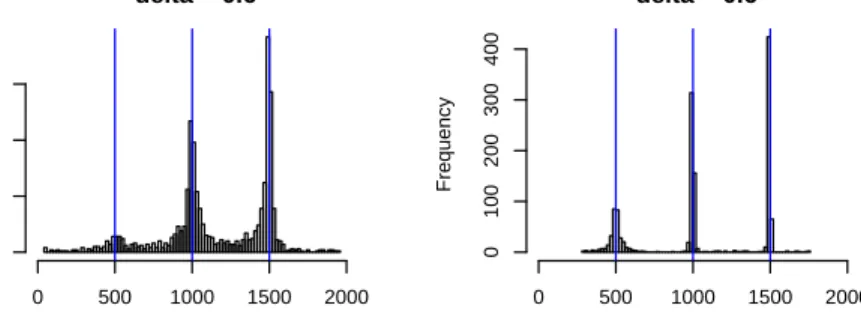
2.8 Histograms of estimated change point locations in complete-overlap structure. Parameters n= 2000, p= 200,(m1, m2, m3) = (500,1000,1500),(||δ (1) n ||2,||δ (2) n ||2,||δ (3) n ||2) = (0.6,1.2,1.8). 39 2.9 Selected plots in comparing bootstrap rejection ˆR(α) v.s. level α for our block Gaussian multiplier bootstrap test underH0. Here,n= 500,p= 600 and the boundary removal is 40. 40 2.10 Selected ˆR(α) plots for block-wise bootstrap testing in [65] underH0. Here,n= 500, p= 600, the boundary removal is 40, ˆσ2 h = σ 2 h and ξl = 1 is used in conditional long-run variance estimators ˆs2 h in bootstrap. The legend is the same as in Figure 2.9. . . 40

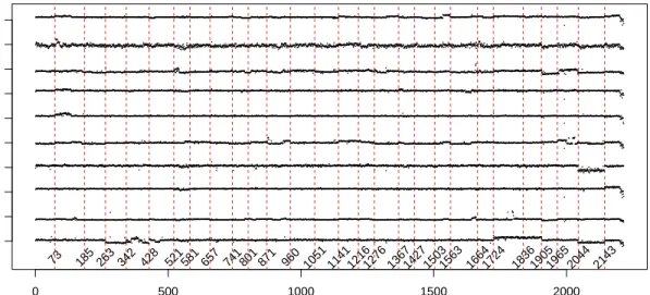
2.11 RMSEs v.s. signal size |δn|∞ for our algorithm (left), [99] (middle) and [37] (right). Here, n= 500, p= 600 and data are from ctm-Gaussian distribution with covariance Vi,j= 0.8|i−j|. 41 2.12 Real data study: aCGH data. Here, we setB = 1000, α= 0.05 and the boundary removal is 60. . . 42

2.13 Selected stock trends. . . 43

2.14 Finance data analyzed by extension of BABS using block CUSUM bootstrap test and two different location estimators. . . 44

2.15 Same setting as in 2.5(b) exceptα= 0.01. . . 78

3.1 Selected setups for comparing ˆR(α) along withα. See headlines for corresponding distribution and kernel. . . 100

3.2 Selected setups for comparing power curves. See headlines and legends for corresponding distribution, kernel, covariance structures and change point locationm. . . 101

3.3 Multiple change point setup using linear kernel at signal level δ = 0.822,10.023. Upper: 2 change points (m1, m2) = (300,600). Lower: 3 change points (m1, m2, m3) = (300,600,800). . 104

3.4 Multiple change point setup using sign kernel at signal level δ = 0.822,10.023. Upper: 2 change points (m1, m2) = (300,600). Lower: 3 change points (m1, m2, m3) = (300,600,800). . 105

3.5 Multiple change point setup using M = 1 and linear kernel at signal level δ= 0.317,2.004. Upper: 2 change points (m1, m2) = (300,600). Lower: 3 change points (m1, m2, m3) = (300,600,800). . . 106

3.6 Trend ofYi= P101 j=1Xij for Enron email dataset. . . 107

(12)

Chapter 1

Introduction

In the era of “Big-Data”, structure heterogeneity issue has received enormous attention in various scientific and engineering fields with application to stock market analysis, quality control, genomics detection and many others. Let Xi ∼Fi, i= 1, . . . , nbe a sequence of independent random vectors taking values in Rp.

In general, the question of change-point analysis in high-dimension arises in the following statistical testing:

H0:F1=· · ·=Fn,

H1:F1=· · ·=Fm1 6=Fm1+1=· · ·=Fm2 6=Fm2+1=· · ·Fmν 6=Fmν+1=· · ·Fn,

for some unknown ν ∈N+ and change point locations 1 < m1 <· · · < mν < n. The structural stability

problem usually can be boiled down to single change point case of ν = 1 (so-called at-most-one-change problem) and extension to multiple change points. The stream to tackle single change point case starts from univariate Gaussian distributed{Fi}n=1that have mean shift [32] or variance shift [25] or both [60] and then to a generalization to location and scale parameters shift [102]. Non-parametric approach such as U-statistics or KolmogorovSmirnov type statistic and semi-parametric approach using empirical likelihood are studied in univariate case [84, 24, 82, 112]. In multivariate setup, we refer to [38] for a rigorous and comprehensive study on the likelihood approach and non-parametric approaches for the aforementioned testing as well as in broader regression and time series models together with sequential methods.

Recently, due to the explosive data enrichment in modern applications where the number of variablesp

is comparable to or even much larger than the sample size n, classical methods are typically inapplicable and the asymptotic theories developed for a fixed dimension do not generally hold. For example, suppose

{Fi}ni=1are Gaussian distribution with meanµiand covariance Σ. Without loss of generality, we may assume

µ1=0. Under the single change point scenario, the log-ratio of the maximized likelihoods betweenH1 with a change point ats= 1, . . . , n−1 andH0 is

(13)

where Zn(s) = r s(n−s) n 1 s s X i=1 Xi− 1 n−s n X i=s+1 Xi ! (1.2) are the cumulative sum (CUSUM) statistics [38], a sequence of the normalized mean differences before and after s. Then H0 is rejected if max16s<nlog(Λs) is larger than a critical value. If s is restricted

to only one location, i.e., the change point location is known, then the problem reduce to a multivariate two-sample mean test that can be solved by Hotelling’s T-squared statistic T2 ₌_Z

n(s)>Σˆ−1Zn(s) where ˆ Σ = _s₋1₁Ps i=1(Xi −X¯ − s)(Xi −X¯s−)T + 1 n−s−1 Pn i=s+1(Xi −X¯ + s )(Xi−X¯s+)T for p < s < n−p and ¯ X_s− = s−1Ps i=1Xi and ¯X + s = (n−s)−1 Pn

i=s+1Xi. In the high-dimensional setting (i.e. p n), ˆΣ, estimation of Σ, itself becomes a challenging problem. The spectral norm consistency of Σ (or the inverse Σ−1) is only possible under additional structural assumptions (such as sparsity or low-rankness) on the covariance matrix [16, 17, 22, 23, 30, 11], which may be violated in practical applications. In contrast, tests based on the CUSUM statistics in (1.2) do not involve Σ and they are more robust to the misspecification on covariance structures. Therefore, this motivates us to study the problems of change point testing and estimation based on the high-dimensional CUSUM statistics.

Although extensive research have been conducted on CUSUM approaches, there is still a number of attracting questions in high-dimension including:

1. How to obtain the distribution of the CUSUM statistics when Gaussianity is violated? 2. What range canstake in both testing and estimation?

3. Is it possible to generate mean test to a broader context?

4. How robust an algorithm/approach can be in terms of various aspects?

For the first question, bootstrapping becomes an option to retrieve latent information and calibrate unknown distribution{Fi}n=1. A large volume of papers studied the performance of resampling bootstrap [12], weighted bootstrap [50] and multiplier bootstrap [21, 20, 42, 65], where the last technique especially enjoys the convenience of maintaining sequence structure in change point analysis. For the second question, it should be noted that boundary changes that happen close to end points of 1 ornare hard to detect due to insufficient data points in one population. Under H0, asymptotic theories allows/n ∈(0,1) [38]. But the connection between signal of change inFi and detectable range is implicit and not clearly stated. The third and fourth

questions are practical concerns when outlier exists, distributional assumption is not satisfied or Fi may

(14)

a fundamental problem therein is to integrate changes carefully and determine relative thresholds properly for the sake of testing and estimation.

In this dissertation, we study finite sample change point detection for high-dimensional data using mul-tiplier bootstraps. Specifically, we propose two `∞-type of statistics based on CUSUM statistics and U-statistics, respectively, to deal with change in mean vector and location parameter. Both of them focus on sparse change that may occur in a small subset of dimension coordinates ofXi at an unknown locationm1.

The four motivating questions will be answered in the perspective of methodology and theory.

1.1 Change point in mean vector and our contributions

In the first part of my dissertation, we focus on inference and identification for structural stability in mean vector using CUSUM statistics. CUSUM statistics have been widely used with a long history pioneered by [83] and followed by two lines in literature: sequential detection foronline change [31, 57, 68, 85] and fixed sample size tests and estimation for offline change [104, 24, 90], latter of which is the core point of interest in this dissertation. Let {Fi} be a location family such that Fi(x) = F1(x−µi). In recent development

for high-dimensional data, testing and estimation for mean-shift are the most intrinsic questions that have been studied in [43, 65] and in [37, 65, 99, 36], respectively. Among them, [43] restricted on testing for Gaussian distribution with diagonal covariance matrix, [99] considered estimation under the same setting and advanced in extension on temporal and spacial dependence with a brief discussion, [37, 65, 36] considered time series sequence and introducedboundary removal concepts without explicit analysis, only [65] provided asymptotic consistency of the bootstrap procedure.

1.1.1 Bootstrapped CUSUM test for single change point

Starting from the simplest single mean-shift model (where data-generating mechanism produces indepen-dent Xi with mean change at most once), we propose a testing procedure based on the test statistic

Tn = maxs6s6n−s|Zn(s)|∞, which aggregates mean-shift signals over sample sequence and targets to the

maximum change across coordinates. To achieve distribution approximation ofTn where observations have

sub-exponential tails or polynomial tails, we apply Gaussian multiplier bootstrap as a computable data-driven approach. Specifically, we define bootstrapped test statistics that capture the distribution of Tn

rather than an upper quantile for a pre-specified significance level. This allows uniform control over size (Type I error). In addition, power can be guaranteed when signal size of change is beyond a lower bound that achieves minimax rate for sparse alternatives. The proposed test is fully data-dependent with no tuning

(15)

parameter except for the boundary removal parameters. Under mild distributional conditions, we demon-strate theoretical requirement on s to justify the difficulty of detecting boundary changes using CUSUM statistics.

The multiplier bootstrap calibrates distribution ofTnwithout referring to extreme value limiting theories

that is known to be slow [87, 53, 65]. Aside from mild moment conditions, no structural condition (in contrast with [43, 99]) nor upper bound ofspatial correlation (in contrast with [36, 65]) oncross-sectional covariance matrix is assumed. So our approach is robust to (i) any distributions that have sub-exponential or polynomial tails, (ii) any correlation among coordinates especially heavy dependence (see simulation). In addition, the dimensionponly affect thesthrough log(np). The searching boundarys(orn−s) is no longer polynomially bounded away from the two endpoints unlike the works [37, 36].

1.1.2 CUSUM based estimators for single change point

As a parallel problem to inference, we continue to study the identification issue and propose two consistent change-point estimators based on CUSUM statistics with two different weights over data sequence. One estimator is covariance stationary and related toTn. The other one provides the best possible convergence

rate ofn−1up to logarithm factors ofnp. We establish non-asymptotic consistency for both estimators that allowpgrows sub-exponentially fast innand can search over the whole data sequence. In application, they can also be tailored to truncated versions in order to adapt to the boundary removal concept in testing. Again, they are robust to distributional tails and spatial correlations that are mentioned above.

1.1.3 Algorithm for multiple change points

Despite the simplicity in single change-point problem for independent data, the appealing properties men-tioned above can extend to multiple change-point scenarios where temporal dependence may exist. For multiple change-point analysis of independent data, binary segmentation [45] is a natural technique to re-cursively test and estimate change points in segments before and after a claimed change point. We propose bootstrap-assisted binary segmentation(BABS) that combines our test and estimators to consistently search and locate change points until nothing shows significance. To accommodate time-series, a block multi-plier bootstrap under single change-point scenario is designed empirically and can be combined with binary segmentation as well.

We would like to emphasize that BABS inherits the robustness from both lines of testing and estimation without introducing additional tuning parameters, and we derive the consistency theoretically. We answered the four questions by

(16)

1. dealing with broader distributions with sub-exponential and polynomial tails rather than Gaussian distribution;

2. deriving explicit rate on boundary removal parameters;

3. discussing a natural extension to detect covariance change point for sub-Gaussian Fi;

4. relaxing weakly dependent requirement for the covariance ofFi.

To relate our work with [65, Bootstrap I and Bootstrap II], which need estimation of single change point prior to testing, our BABS is designed reversely (or say simultaneously). Arithmetically, testing and estimation are two separate problems that should be able to conduct independently. However, in [65], (long-run) covariance estimators for each coordinates must be normalized according to a possible change point before performing bootstrapping under single alternativeH1. Though, [65, Bootstrap III] proposed a “naive” way to entirely remove the estimation of change point in bootstrap under H1, their test statistic [65, Eq (1.2)] still relies on (long-run) covariance estimators. Therefore, there is a fundamental difficulty to extend their approach for a global detection of multiple change points except to, for instance, apply wild bootstrap technique [45] with sacrifice on computation cost. Thus, our BABS is more aligned with statistical philosophy with no additional estimation step nor threshold selection that of vital importance to other multiple change point estimation algorithms [37, 99, 36].

1.2 Change point in location parameter and our contributions

In the second part, we consider the class of distribution where mean vector is not well-defined. Recall the location-shift model such that Fi(x) = F1(x−µi). When it comes to i.i.d. observations whose latent

distribution is from a heavy-tailed location family that does not have finite mean, CUSUM-type approaches will fail due to violation on moment conditions. As a consequence, a non-linear projection of data must be imposed to separate H0 (no change point) andH1 (at most one location shift over the sequence of data). This motivates us to investigate new technique for high-dimensional robust change-point analysis.

U-statistics, which sum up all permutations of samples filtered by a kernel, produce robust and unbiased estimation of the kernel function after proper normalization. Such function must be selected properly in order to reflect changes in location parameter. In the common choice of symmetric ones, high-order kernels (e.g. in order-four) have been designed to cancel out within-sample means or location parameters [38, 97]. On the other hand, if the single change point is assumed known to be s, the problem falls to investigation of two-sample (before and afters) U-statistics that can separate between-sample difference. Then a natural

(17)

extension for unknown change point case is to take the test statistic as the maximum of between-sample differences over s = 1, . . . , n−1 [25, 77, 73, 52, 40]. However, such modifications are computationally expensive to cancel out noises by lifting to high-order kernels and unnecessary to screen whole sequence for testing only and no intention on estimation.

To remedy the issue of robustness and efficiency, we propose a novel `∞-type testing statistic based on one-sample order-two U-statistics coupled with anti-symmetric kernels in Chapter 3. Specifically, our statistic is defined as Tn=n1/2 _n 2 −1 X 16i<j6n h(Xi, Xj) (1.3) where h : _Rp_×

Rp → Rd is an anti-symmetric kernel, i.e., h(x, y) = −h(y, x) for all x, y ∈ Rp, which

plays a key role in testing. Under the null H0, the mean of Tn is always 0, while under the alternative

H1, the within-sample noise cancels out and the between-sample signal is properly preserved by kernel. In the perspective of computational cost, the general order is O(n2_p_{) for the example of robust sign-kernel}

h(x, y) =sign(x−y) (component-wise) and it can be reduced toO(np) by using the one-pass linear-kernel

h(x, y) =x−y.

Our proposed U-statistics approach is robust, tuning-free and easy-to-implement. Gaussian multiplier bootstrap is designed to calibrate the distribution of test statistic. Subject to mild moment conditions on kernels, we derive the uniform rates of convergence for distribution approximation and the lower bound of location-change signal through kernel. It should be noted that no boundary removal procedure is required since the one-sample U-statisticTn integrates “two-sample” information without referring each data point.

We can answer the four questions raised in the beginning by

1. considering kernel projection to release distributional assumption; 2. performing global testing without boundary removal;

3. leaving possibility of other tests to choices of kernelh;

4. extending to location parameter ofFi which is not necessary to have mean.

In the presence of multiple change points, the U-statistic based test is valid if location shifts accumulate ideally. Since the signal cancellation may nullify power, a block testing is designed to gain single change point structure with sacrifice of sample size. Due to the advantage that our test does not screen any difference before and after each point, it limits to extend the test statistic to a change point estimator as in the CUSUM-based approach. As a consequence, the binary segmentation CUSUM-based forward detection cannot directly apply to our framework. However, a backward searching algorithm (BD) can play a role of estimation without

(18)

introducing external estimator. Specifically, BD repeatedly merges two consecutive data segments whose union fail to rejectH0. Therefore, it is more powerful especially when there are short sequences with location shifts.

The rest of this dissertation is organized as follows. The CUSUM based test and estimator together with the BABS algorithm for mean change are elaborated in Chapter 2 [106]. The U-statistics based test as well as the BD algorithm is described in Chapter 3 [107]. Main results, numerical studies and proofs are given within each chapter, respectively.

(19)

Chapter 2

Change point inference and

identification for high-dimensional

mean vectors

2.1 Introduction

This paper studies the problems of change point inference and identification for mean vectors of high-dimensional data in finite samples. High-high-dimensional data are now ubiquitous in many scientific and engi-neering fields and data heterogeneity is the rule rather than the exception. A central problem of studying the data heterogeneity is to detect structural breaks in the underlying data generation process. Perhaps the two most fundamental questions for abrupt changes are: i) is there a change point in data? ii) if so, when does the change occur? In this work, we consider change point detection and identification for temporally independent data with cross-sectional dependence. Specifically, let Xn

1 ={X1, . . . , Xn} be a sequence of

independent random vectors in_Rp_{generated from the mean-shift model:}

Xi=µ+δn1(i > m) +ξi, i= 1, . . . , n, (2.1)

where µ ∈ Rp is the population mean parameter, δn ∈ Rp is the mean-shift signal parameter, m is the

change point location, andξ1, . . . , ξnare (temporally) independent and identically distributed (i.i.d.)

mean-zero noise random vectors in Rp with common distribution functionF. Let Σ = Cov(ξ1) be the unknown

noise covariance matrix that is not necessarily diagonal, and thus we allow cross-sectional (sometimes also referred as spatial) dependence among the componentsXi1, . . . , Xip for each i= 1, . . . , n. Under the

mean-shift model, if δn = 0 or m =n, then X1, . . . , Xn form a sample of i.i.d. random vectors and no change

point occurs. In this paper, our first goal is to test for whether or not there is a change point in the mean vectorsµi=E(Xi), i.e., to test for

H0:δn= 0 and H1:δn6= 0 and there exists anm∈ {1, . . . , n−1}, (2.2)

where the alternative hypothesis H1 is parameterized by the change point signal δn and location m. If a

(20)

change point locationm.

For i.i.d. Gaussian noise ξi ∼ N(0,Σ), the log-ratio of the maximized likelihoods between H1 with a change point ats= 1, . . . , n−1 andH0 without change point is given by

log(Λs) =Zn(s)>Σ−1Zn(s)/2, (2.3) where Zn(s) = r s(n−s) n 1 s s X i=1 Xi− 1 n−s n X i=s+1 Xi ! (2.4) is a sequence of the normalized mean differences before and afters. ThenH0is rejected if max16s<nlog(Λs)

is larger than a critical value. In literature, {Zn(s)}ns=1−1 are often called the cumulative sum (CUSUM) statistics [38]. Note that the log-ratio statistics of the maximized likelihoods in (2.3) require the knowledge or an estimate of the unknown covariance matrix Σ. In the high-dimensional setting where p is larger (or even much larger) than n, estimation of Σ itself becomes a challenging problem. And the spectral norm consistency of Σ (or the inverse Σ−1_{) is possible under additional structural assumptions (such as} sparsity or low-rankness) on the covariance matrix [16, 17, 22, 23, 30, 11], which may be violated in practical applications. In contrast, tests based on the CUSUM statistics in (2.4) do not involve Σ and they are more robust to the misspecification on covariance structures. Therefore, this motivates us to study the problems of change point testing and estimation based on the high-dimensional CUSUM statistics.

To build a decision rule for change-point detection, we need to cautiously aggregate the (dependent) random vectorsZn(s), s= 1, . . . , n−1. [43] considers the change point detection on mean vectors under the

mean-shift model (2.1) with i.i.d.ξi∼N(0, σ2Ip). They propose the linear and scan statistics based on the`2

-norm aggregation of the CUSUM statistics and derive the change point detection boundary. [65] considers the

`∞_{-norm aggregation of the CUSUM statistics and establishes a Gumbel limiting distribution under}_H

0. [65] also considers the bootstrap approximations to improve the rate of convergence. [99] considers the estimation problem of change points in the high-dimensional mean vectors in reduced dimensions by sparse projections and they derive the rate of convergence for estimating the change point location. In all aforementioned papers [43, 65, 99], strong structural assumptions (i.e., cross-sectional sparsity in the sense that the components

{Xij}pj=1 of Xi are independent or weakly dependent) are imposed to substantially reduce the intrinsic

complexity of the problem. [37] relax the sparsity assumption and consider the estimation problem of change points in the (marginal) variances of high-dimensional time series under a multiplicative model. They propose asparsified binary segmentation(SBS) performing the`1-norm aggregation on a thresholded version of the CUSUM statistics such that an additional sparsifying step with a tuning parameter is used to

(21)

avoid noise accumulation in the aggregation. Since the SBS is sensitive to threshold tuning parameters, [36] proposes a double CUSUM test procedure sorting the magnitudes of thepcomponents of CUSUM statistics and it may be viewed as a data-driven alternative for selecting the threshold in [37].

In this paper, besides some mild moment conditions, we do not make any assumption on the cross-sectional dependence structure of the underlying data distribution. We consider the multivariate CUSUM statistics (2.4) in the`∞-norm aggregated form:

Tn= max

s6s6n−s|Zn(s)|∞:=s6maxs6n−s1max6j6p|Znj(s)|, (2.5)

where s∈[1, n/2] is a user-specifiedboundary removal parameter. Removing boundary points is necessary in detecting a change point since the distributions of |Zn(s)|∞ that are closer to the endpoints are more

difficult to approximate because of fewer data points. ThenH0is rejected ifTnis larger than a critical value

such as the (1−α) quantile ofTn. UnderH0,{Zn(s)}ns=1−1is a centered and covariance stationary process in

Rp (i.e., E[Zn(s)] = 0 and Cov(Zn(s)) = Σ). To approximate the distribution ofTn, extreme value theory

is a commonly used technique to derive the Gumbel-type limiting distributions [69, 87]. However, even in

p= 1 case, the convergence rate of maxima of the CUSUM process{Zn(s)}ns=1−1 is known to be very slow [87, 53, 65].

2.1.1 Our contributions

To overcome the fundamental difficulty in calibrating the distribution of Tn, we consider the bootstrap

approximation to the finite sample distribution of Tn without referring a weak limit of {Zn(s)}ns=1−1. In Section 2.2, we propose a Gaussian multiplier bootstrap tailored to the CUSUM test statistics in (2.4). The proposed bootstrap test is fully data-dependent and requires no tuning parameter (except for a pre-specified boundary removal parameters). This is in contrast with the thresholding-aggregation method in [37], which requires further data-dependent procedures to choose the threshold and is not easy to justify. We will show in Section 2.3.1 that the bootstrap CUSUM test is a uniformly valid inferential procedure underH0 where

p can grow sub-exponentially fast in n andno explicit condition on the dependence structure among the components{Xij}

p

j=1is needed. This is in contrast with [43, 65, 99] where the components are assumed to be either independent or weakly dependent, and with [37, 36] where the dimension can only grow polynomially fast in sample size. Moreover, we will show that, under a mild signal strength condition, our bootstrap CUSUM test is consistent in the sense that the sum of type I and type II errors is asymptotically vanishing [47, Chapter 6.2]. In addition, the requirement on the signal strength can achieve the minimax separation

(22)

rate derived in [43] under the sparse alternative (i.e., the change occurs only in a few number of components

X1, . . . , Xn).

If a change point is detected, then we estimate the change point location by maximizing the`∞-norm of the generalized CUSUM statistics (2.8) at two different weighting scales. The first estimator is based on the covariance stationary CUSUM statistics in (2.4). In Section 2.3.2, we show that it is consistent in estimating the location at the parametric raten−1/2 _{(up to logarithmic factors) for sub-exponential observations. The} second estimator is a non-stationary CUSUM statistics assigning less weights on the boundary data points. In this case, we show that it achieves the best possible rate of convergence on the ordern−1_{(up to logarithmic} factors) under some stronger side conditions. In both cases, dimension impacts the rate of convergence only through the logarithmic factors. Thus consistency of the CUSUM location estimators can be achieved when

pgrows sub-exponentially fast inn.

Our bootstrap change point inference can be naturally extended to handle multiple change points via the generic binary segmentation technique. Once a change point is claimed by our bootstrap test and located in the estimation step, the binary segmentation continues the same testing and estimation procedure on the segments before and after the change until no further change point can be detected by the bootstrap test (cf. Algorithm 1 in Section 2.2.3). Thus, the bootstrap CUSUM test can dynamically adjust the detection rule during the iterations. We derive the rate of convergence of this bootstrap-assisted binary segmentation (BABS) for recursively estimating the multiple change points under suitable signal separation and strength conditions. No additional tuning parameter is introduced in BABS.

2.1.2 Literature review

CUSUM statistics [83] are originally introduced in the sequential testing problems to distinguish between the in-control hypothesisδn= 0 and the out-control mean-shift hypothesis for agivenδn6= 0 in model (2.1),

aiming to minimize the expected average run length [68, 94, 95, 83, 31, 57, 101, 95, 76, 85]. This paper uses CUSUM statistics for fixed sampled size tests, as in many other statistical change point testing and estimation works [104, 19, 38, 67, 13, 45, 24, 75, 55, 54, 44, 46, 81, 8, 9, 15, 109, 56].

There is a recent surge of literature on change point analysis for high-dimensional data. Change point detection is considered in [43, 65]. Estimation of the number and locations of change points are considered in [37, 65, 99, 36]. Bootstrap inference is considered in [36] (without rigorous statistical guarantees).

Finite sample approximations to the distribution of maxima corresponding to sums ofindependent mean-zero random vectors in high dimensions are studied in [33, 35]. We highlight that validity of our bootstrap CUSUM test for the change point does not (at least directly) follow the Gaussian and bootstrap

(23)

approxima-tion results in [33, 35]. The reason is that, in the change-point detecapproxima-tion context, the extreme-value type test statisticTndefined in (2.5) is the maximum of a sequence ofdependentrandom vectorsZn(s), s=s, . . . , n−s.

Therefore, the distributional approximation results developed in [33, 35] require considerable modifications tailored to the change point analysis. A main technical innovation of this work is that the CUSUM statistics are affine transformations of the independent data points in an augmented space so that we can make use of the high-dimensional Gaussian and bootstrap approximations without overpaying the price of the increased dimensionality in the embedded larger space.

2.1.3 Organization

The rest of this paper is organized as follows. The bootstrap change point test, estimation of the change point location and extension to multiple change point algorithm are described in Section 2.2. In Section 2.3, we derive the size validity, power properties of the bootstrap test and the rate of convergence for the change point location estimator by the generalized CUSUM statistics, followed by consistency of algorithm designed for multiple change point identification. In Section 2.4, we report extensive simulation results of testing and estimation for a variety of distributions with different dependence structures and moment conditions. In Section 2.5, real data examples are provided. Proofs of the main results in Section 2.3 and additional simulation results are given in Section 2.6.

2.1.4 Notation

Forq >0 and a generic vectorx∈Rp, we denote |x|q = (P p

i=1|xi|q)1/q for the`q norm ofxand we write

|x| = |x|2. For a random variable X, denote kXkq = (E|X|q)1/q. For β > 0, let ψβ(x) = exp(xβ)−1

be a function defined on [0,∞) and Lψβ be the collection of all real-valued random variables X such that E[ψβ(|X|/C)]<∞for someC >0. ForX ∈Lψβ, definekXkψβ = inf{C >0 :E[ψβ(|X|/C)]61}. Then,

forβ∈[1,∞),k · kψβ is an Orlicz norm and (Lψβ,k · kψβ) is a Banach space [70]. Forβ∈(0,1), k · kψβ is a

quasi-norm, i.e., there exists a constantC(β)>0 such thatkX+Ykψβ 6C(β)(kXkψβ+kYkψβ) holds for

allX, Y ∈Lψβ [1]. Letρ(X, Y) = supt∈R|P(X 6t)−P(Y 6t)|be the Kolmogorov distance between two random variablesX andY. We shall useC1, C2, . . . andK1, K2, . . . to denote positive and finite constants that may have different values. Throughout the paper, we assumen_>4 andp_>3.

(24)

2.2 Methodology

2.2.1 Bootstrap CUSUM test

We first introduce a bootstrap procedure to approximate the distribution ofTn. Lete1, . . . , enbe i.i.d.N(0,1)

random variables independent of X1, . . . , Xn. Let ¯Xs− =s−1

Ps

i=1Xi and ¯Xs+ = (n−s)−1

Pn

i=s+1Xi be

the left and right sample averages ats, respectively. Define

Z_n∗(s) = r n−s ns s X i=1 ei(Xi−X¯s−)− r _s n(n−s) n X i=s+1 ei(Xi−X¯s+). (2.6)

Then the bootstrap test statistic is defined as

T_n∗= max

s6s6n−s|Z

∗

n(s)|∞, (2.7)

and the (1−α) conditional quantile ofT_n∗ givenXn

1 qT∗ n|Xn1(1−α) = inf{t∈R:P(T ∗ n 6t|X n 1)>1−α}

is used as a critical value of the bootstrap test to approximate the quantiles of Tn. In particular, for any

α∈(0,1), we rejectH0ifTn> qT∗

n|X1n(1−α). Note that the Gaussian multiplier bootstrap test statisticT

∗

n

and its conditional quantileqT∗

n|X1n(1−α) arecomputablein the sense that we can repeatedly draw Monte Carlo samples by simulating the multiplier random variables e1, . . . , en to approximate the distribution of

T_n∗.

Remark 1 (Comments on centering in the bootstrap CUSUM statistics Z_n∗(s)). Alternatively, we can also consider the following version of bootstrap CUSUM statistics

˜ Z_n∗(s) = r n−s ns s X i=1 eiXi− r _s n(n−s) n X i=s+1 eiXi

without left and right centering by ¯X_s− and ¯X+

s. It can be shown that the bootstrap CUSUM test based on

(25)

and Theorem 2.3). However, Cov(Z_n∗(s)|X₁n) = n−s ns s X i=1 (Xi−X¯s−)(Xi−X¯s−)>+ s n(n−s) n X i=s+1 (Xi−X¯s+)(Xi−X¯s+)> 6 n−s ns s X i=1 XiXi>+ s n(n−s) n X i=s+1 XiXi> = Cov( ˜Zn∗(s)|X n 1),

where we write two square matricesA₆B ifA−B₆0 i.e.,A−B is negative semi-definite. Hence ˜Z_n∗(s) incurs a larger (conditional) covariance matrix thanZ_n∗(s) and it is recommended to useZ_n∗(s) rather than

˜

Z_n∗(s).

Remark 2 (Comparisons with [65] under H0). In a related work, [65] considers the change point tests for high-dimensional time series based on the following version of the CUSUM statistics

Bnj = 1 ˆ σj √ n1max6s6n s X i=1 Xij− s n n X i=1 Xij , j= 1, . . . , p,

where ˆσ2_j is a consistent estimator for the long-run variance of {Xij}i∈N. Then H0 is rejected if ˜Tn =

max16j6pBnj is larger than a critical value. Under H0 and the spatial sparsity conditions (Assumption 2.2 in [65]), the author establishes a Gumbel limiting distribution for ˜Tn (after suitable normalizations).

To improve the rate of convergence, the author also proposes a parametric bootstrap ˜TY

n = max16j6pBnjY , where B_njY =√1 n1max6s6n s X i=1 Yij− s n n X i=1 Yij , j= 1, . . . , p,

and{Yij: 16i6n,16j6p}is an array of i.i.d.N(0,1) random variables. Asymptotic bootstrap validity

is derived under the same spatial sparsity assumption as in the Gumbel limit. There is an important difference between ˜TnY in [65] and our bootstrap test based on Tn∗. Note that the conditional covariance matrices of

Zn∗(s) given X1n are sample analogs of covariance matrices of Zn(s). We will show in Section 2.3.1 that

T∗

n can approximate the distribution of Tn without assuming any kind of spatial (cross-sectional) sparsity

conditions. On the contrary, since {Yij} are i.i.d., even when X1, . . . , Xn are independent observations,

the parametric bootstrap BY

nj does not mimic the general dependence structure among the components

{Xij}pj=1. In addition, the bootstrap validity ofTn∗ we establish in Theorem 2.1 and Corollary 2.2 below is

(26)

2.2.2 Estimating the change point location under the alternative hypothesis

If a change point is detected in the mean vectors (i.e.,H0 is rejected), then our next goal is to identify the change point locationm. Specifically, we estimate tm=m/n, m= 1, . . . , n,where the data X1, . . . , Xn are

observed at evenly spaced time points and their index variables are normalized to [0,1]. We consider the change point location estimator based on the generalized CUSUM statistics [55]

Zθ,n(s) = _s₍_n −s) n 1−θ 1 s s X i=1 Xi− 1 n−s n X i=s+1 Xi ! , (2.8)

whereθ is a weighting parameter satisfying 0₆θ <1. Obviously, the CUSUM statisticsZn(s) in (2.4) is a

special case ofθ= 1/2, i.e.,Zn(s) =Z1/2,n(s). Then we estimate mby

ˆ

mθ= argmax16s<n|Zθ,n(s)|∞. (2.9)

and we use tmˆθ = ˆmθ/n to estimatetm. It is easily seen that, for smaller values ofθ, Zθ,n(s) assigns less

weights on the boundary data points. Therefore, if the true change point location is bounded away from the two endpoints, we expect thattmˆθ with a smaller weighting parameter can achieve better rate of convergence.

For example, iftm∈(0,1) is fixed andp= 1, then it is known that the{Z0,n(s)}ns=1−1 converges weakly to a functional of the Weiner process and the corresponding maximizer ˆm0achieves the rate of convergence of the ordern−1, which is clearly the best possible rate and is faster than the parametric raten−1/2[9, 55]. Instead of considering the whole family of the generalized CUSUM statistics indexed byθ∈[0,1), we consider two important cases ofθ = 1/2 (covariance stationary) andθ= 0 (non-stationary) in this paper. For θ= 1/2,

Z1/2,n(s) is related to the proposed bootstrap CUSUM statisticsZn∗(s) in (2.6) and the log-ratio statistics

in (2.3) under normality with Σ =σ2_Id

p. Forθ= 0,Z0,n(s) is related to the parametric bootstrap in [65].

Remark 3 (Comments on the boundary). It should be noted that in the bootstrap CUSUM test, we must remove the boundary points from approximating the distribution ofTn. If the boundary points are included

in the maximaTn andTn∗, then the conditional distribution ofTn∗ (givenX n

1) does not provide an accurate approximation to the distribution of Tn. Theorem 2.1 and Theorem 2.3 provide the precise rate of

conver-gence that characterizes the boundary removal parameters to ensure the consistency (in terms of the sum of type I and type II errors) of the bootstrap CUSUM test. On the other hand, the estimation problem in (2.9) does not exclude the endpoints outside the interval [s, n−s]. However, in practice, if the existence of a change point is not known as a priori and it is decided by a test, then the boundary restriction is implicitly imposed for both testing and estimation in empirical applications [9].

(27)

2.2.3 Bootstrap-assisted binary segmentation for multiple change points

Suppose now there are ν change pointsm0 = 1< m1 <· · ·< mν < mν+1 =nand consider the following multiple mean-shifts model:

Xi=µ+ ν

X

k=1

δ_n(k)1(i > mk) +ξi, i= 1, . . . , n, (2.10)

where δn(k) ∈ Rp are non-zero mean-shift vectors and ξi are again i.i.d. mean-zero random vectors in Rp.

Without less of generality, we may assumeµ= 0 andδ(0)n =δ(nν+1)= 0. Given a beginning time pointband

an ending time pointe, we can compute the CUSUM statistics on the initial data segment{Xi}ei=b:

Zn,b,e(s) = r (s−b+ 1)(e−s) e−b+ 1 1 s−b+ 1 s X i=b Xi− 1 e−s e X i=s+1 Xi ! .

Note that the normalization inZn,b,e(s) corresponds to the caseθ= 1/2 in (2.8). It can be shown that the

maximizer of|_EZn,b,e(s)|∞, s=b, . . . , ealways occurs at one of the change points{mk, k= 1, . . . , ν} ∩[b, e]

(cf. Lemma 2.13). Therefore, under multiple change points model (2.10), we can useZn,b,e(s) to locate one

shift in the interval [b, e]. If our bootstrap CUSUM test (calculated based on {Xi}ei=b) rejects H0 at the significance levelα, then ˆme

b = argmaxs=b,...,e|Zn,b,e(s)|∞is marked as a change point. In addition, observe

that the mean vectorsµi=E[Xi] are piecewise constant such that

µmk+1=· · ·=µmk+1=

k

X

l=0

δ(_nl).

Thus, we may recursively apply the binary segmentation to search along the two directions [b,mˆe b] and

[ ˆme

b+ 1, e] until no further change point would be detected by the subsequent bootstrap tests. The

pseudo-code for our bootstrap-assisted binary segmentation algorithm for multiple change points detection, referred as BABS(α, b, e), is summarized in the following Algorithms 1.

2.3 Theoretical results

(28)

Algorithm 1BABS(α, b, e)

1: if e−b+ 1<2sthen

2: STOP

3: else

4: mˆe_b = argmaxs=b,...,e|Zn,b,e(s)|∞

5: if our bootstrap CUSUM test concludes existence of a change in [b, e]then 6: add ˆme

b to the set of estimated change-points;

7: BABS(α, b,mˆe b); 8: BABS(α,mˆe b+ 1, e). 9: else 10: STOP 11: end if 12: end if

13: return estimated change points.

2.3.1 Size and power of the bootstrap CUSUM test: one change point

Our first main result (cf. Theorem 2.1) is to establish finite sample bounds for the (random) Kolmogorov distance betweenTn andTn∗:

ρ∗(Tn, Tn∗) = sup t∈R

|P0(Tn6t)−P0(Tn∗6t|X

n

1)|.

From this, we can derive the asymptotic bootstrap validity for certain high-dimensional scaling limit for (n, p). In particular, with ρ∗(Tn, Tn∗) = oP(1), we can show that Type-I error of the bootstrap test is

asymptotically controlled at the exact nominal level α ∈ (0,1); i.e., _P0(Tn > qT∗

n|X1n(1−α)) → α (cf. Corollary 2.2).

Letb,¯b, q >0. We make the following assumptions. (A) Var(ξij)>b for allj= 1, . . . , p.

(B) _E[|ξij|2+`]6¯b` for`= 1,2 and for alli= 1, . . . , nandj= 1, . . . , p.

(C) kξijkψ1 6¯bfor alli= 1, . . . , n andj= 1, . . . , p. (D) _E[max16j6p(|ξij|/¯b)q]61 for alli= 1, . . . , n.

Condition (A) is a non-degeneracy assumption. Condition (B) is a mild moment growth condition. Without loss of generality, we may take ¯b_>1. Conditions (C) and (D) impose sub-exponential and uniform polynomial moment requirements on the observations, respectively. Define

$1,n= _log7₍_np₎ s 1/6 and $2,n= _n2/q_log3 (np) γ2/q_s 1/3 .

(29)

Theorem 2.1(Main result I:bounds on the Kolmogorov distance betweenTnandTn∗underH0). Suppose

H0 is true and assume (A) and (B) hold. Letγ∈(0, e−1)and suppose thatlog(γ−1)6Klog(pn)for some constant K >0.

(i) If (C) holds, then there exists a constant C >0 only depending on b,¯b, K such that

ρ∗(Tn, Tn∗)6C$1,n (2.11)

holds with probability at least 1−γ.

(ii) If (D) holds, then there exists a constantC >0only depending on b,¯b, K, q such that

ρ∗(Tn, Tn∗)6C{$1,n+$2,n} (2.12)

holds with probability at least 1−γ.

Based on Theorem 2.1, we have the uniform size validity of the bootstrap CUSUM test.

Corollary 2.2 (Uniform size validity of Gaussian multiplier bootstrap for the CUSUM test). SupposeH0

is true and assume (A) and (B) hold. Let γ ∈ (0, e−1₎ _{and suppose that} _log(_γ−1₎

6 Klog(pn) for some constant K >0.

(i) If (C) holds, then there exists a constant C >0 only depending on b,¯b, K such that

sup

α∈(0,1)

|_P0(Tn6qT∗

n|Xn1(α))−α|6C$1,n+γ. (2.13) Consequently, if log7(np) =o(s), then_P0(Tn6qT∗

n|X1n(α))→αuniformly in α∈(0,1) asn→ ∞. (ii) If (D) holds, then there exists a constantC >0 only depending onb,¯b, K, q such that

sup

α∈(0,1)

|P0(Tn6qT∗

n|X1n(α))−α|6C{$1,n+$2,n}+γ. (2.14) Consequently, if max{log7(np), n2/qlog3+ε(np)} = o(s) for some ε > 0, then _P0(Tn 6 qT∗

n|X1n(α)) → α uniformly in α∈(0,1) asn→ ∞.

Our second main result is to analyze the power of the bootstrap CUSUM test. We are mainly interested in characterizing the change point signal strength (quantified by the`∞norm ofδn) and the locationtmsuch

thatH0andH1 can be asymptotically separated by our bootstrap CUSUM test. Without loss of generality, we may assume that|δn|∞61.

(30)

Theorem 2.3 (Main result II: power of Gaussian multiplier bootstrap for CUSUM test under H1).

SupposeH1 is true with a change point m∈[s, n−s] and assume (A) and (B) hold. Let ζ∈(0,1/2) and

γ∈(0, e−1₎_{such that}_log(_γ−1₎

6Klog(pn)for some constant K >0. (i) If (C) holds and

|δn|∞>C1

s

log(ζ−1_{) log(}_np_{) + log(}_np/α₎

ntm(1−tm)

(2.15) for some large enough constant C1 := C1(¯b, b, K)> 0, then there exists a constant C2 :=C2(¯b, b, K) >0 such that

P1(Tn> qT∗

n|Xn1(1−α))>1−γ−C2$1,n−2ζ. (2.16) (ii) If (D) holds and|δn|∞ obeys (2.15) for some large enough constant C1:=C1(¯b, b, K, q)>0, then there exists a constantC2:=C2(¯b, b, K, q)>0 such that

P1(Tn> qT∗

n|X1n(1−α))>1−γ−C2{$1,n+$2,n} −2ζ. (2.17) Remark 4 (Rate-optimality on the change point detection for sparse alternatives). Under the i.i.d. Gaussian errorsξi ∼N(0,Idp) in the mean-shift model (2.1), the detection boundary for a change point in a Gaussian

sequence is characterized in [43]. Leta >0 and suppose that a change point

δn= (a, . . . , a

| {z }

ktimes

,0, . . . ,0)>

occurs in the firstkcomponents at the locationmin the sequence X1, . . . , Xn. Following [43], we consider

the scaling limitp=nc1 _and_k ₌_p1−c2 _{for some}_c

1>0 and c2 ∈[0,1). Ifc2 ∈(1/2,1), then the number of components with a change point is highly sparse. In this case, the minimax separation condition forH0 andH1 is given by a=rp s log(p) ntm(1−tm) .

Specifically, detection is impossible if lim sup_p_→∞rp <

√

2c2−1 and detection is possible if lim infp→∞rp>

p

2c2/(1−log 2). On the other hand, choosing αn = n−c for some constant c > 0 in Corollary 2.2 and

Theorem 2.3, we see that if

a_>C∗

s

log(ζ−1_{) log(}_p₎

ntm(1−tm)

for some large constant C∗ > 0, then our bootstrap CUSUM change point test achieves the minimax separation rate in the high sparsity regime (with stronger side conditions to ensure the bootstrap validity).

(31)

Hence, the signal strength requirement for detection in the proposed bootstrap test achieves the minimax optimal rate under the sparse alternatives. On the other hand, it should be noted that, under the dense alternativesc2∈[0,1/2], our bootstrap CUSUM test remains consistent in detecting the change point signal in the sense that the sum of type I and type II errors converges to zero. However, in such case, the bootstrap CUSUM test does not reach the detection boundary and the minimax separation rate [43].

Remark 5 (Monotonicity of power in the signal strength). Inspecting the proof of Theorem 2.3, it is seen that the type II error of the bootstrap CUSUM test is bounded by a probability depending on the change point signal strength|δn|∞and locationm(cf. equation (2.44)). Specifically,

Type II error₆_P1( ˜Tn>∆˜ −qT∗

n|X1n(1−α)),

where ˜∆ =pntm(1−tm)|δn|∞, ˜Tn = maxs6n6n−s|Znξ(s)|, andZnξ(s) are the CUSUM statistics computed

on the (unknown)ξn

1 random vectors. Since the distribution of ˜Tndoes not depend onδnand the conditional

quantile qT∗

n|Xn1(1−α) is bounded by O( p

log(np)) with a large probability under H1, the power of the bootstrap CUSUM test is lower bounded by a quantity that is non-decreasing in|δn|∞. Simulation examples

in Section 2.4 confirm our theoretical observation. In addition, sincetm(1−tm) is maximized attm= 1/2,

a change point near the middle is easier to detect than it is near the boundary.

Remark 6 (Choice of boundary removal parameter). There is a trade-off for the choice of boundary removal parameter: the larger s, the smaller of the error bounds and the more data points are removed from the change point detection (so that the regime allowed by the bootstrap CUSUM test is smaller). In theory, the lower bound ofsis given in Corollary 2.2 for size validity of the bootstrap CUSUM test. Specifically, if the data distribution has sub-exponential tail (i.e., Condition (C) holds), then we needslog7(np) for the error-in-size$1,n=o(1); if the data distribution has polynomial tail (i.e., Condition (D) holds) withq >0,

then we need smax{log7(np), n2/q_log3+ε₍_np₎_}_for _$

1,n+$2,n =o(1). This implies that we can choose

s=c1nc2 for some small constantsc1>0,1>c2>0 in either sub-exponential or polynomial case.

As a leading example, we consider a fixed normalized true change point location tm = m/n ∈ (0,1).

Then we may chooses =c0n for some small constant c0 > 0 in order to include the change point in the interval [s, n−s]. Under this framework, asymptotic size validity of the bootstrap CUSUM test is obtained ifp=O(enc) for some 1/7> c >0 under the sub-exponential moment condition on the observations.

Remark 7 (Comparisons with [65] under H1). [65] proposed bootstrap testing procedures for change point under the alternative, which are different from the parametric bootstrap underH0 (cf. Remark 2).

(32)

Specif-ically, the author considers several block versions of the multiplier and empirical bootstraps under H1 in the time series setting. All of the tests under H1 in [65] require a minimum signal strength condition (cf. Assumption 4.3 therein): lim sup n→∞ logn Kbminj∈Sδnj2 = 0, (2.18)

where S ={j ∈ {1, . . . , p} :δnj 6= 0} and Kb is the size of blocks. There are two major differences from

the bootstraps in [65]. First, our Gaussian multiplier bootstrap CUSUM test is asymptotically valid and powerful for a change point under both H0 and H1. On the contrary, [65, Section 4] designed a series estimators of tm to adapt to estimation of ˆσj2, j = 1, . . . , punder H1, and the estimators must rely on the

assumption that each dimension has at most one change point. However, our approach without estimation of

tmcan test against more generalized multiple change-point problem where power can still be guaranteed (cf.

Lemma 2.6). Second, detection by our bootstrap CUSUM test relies on a lower bound on the signal strength quantified by|δn|∞, which is much weaker than (2.18). For example, it is possible that the minimum signal

strength minj∈Sδnj2 decays to zero faster than (logn)/Kb, while our bootstrap CUSUM test remains valid

since it only requires|δn|∞satisfies a mild lower bound in (2.15).

2.3.2 Rate of convergence of the change point location estimator

Our third main result is concerned with the rate of convergence of the change point location estimatortmˆθ,

where ˆmθ is defined through (2.9) and (2.8). We first consider the case of θ = 1/2 corresponding to the

covariance stationary CUSUM statistics.

Theorem 2.4(Main result III:rate of convergence for change point location estimator: θ= 1/2). Suppose

that (B) holds andH1 is true. Suppose thatlog(γ−1)6Klog(np)for some constant K >0. (i) If (C) holds, then there exists a constant C >0 depending only on¯b, K such that

P1 |tmˆ1/2−tm|6 Clog2(np) p ntm(1−tm)|δn|∞ >1−γ. (2.19)

(ii) If (D) holds withq >2, then there exists a constantC >0 depending only on¯b, K, q such that

P1 |tmˆ1/2−tm|6 Cn1/q_(log(_np_{) +}_γ−1/q₎ p ntm(1−tm)|δn|∞ >1−γ. (2.20)

Note that the non-degeneracy Condition (A) is not needed in estimating the change point location. Consider a fixedtm∈(0,1) as in our leading example. It is seen from Theorem 2.4 that tmˆ1/2 is consistent for estimatingtmif the signal strength satisfying: i)|δ|∞n−1/2log2(np) in the sub-exponential moment

(33)

case; ii)|δ|∞n−1/2+1/qlog(np) in the polynomial moment case. From Part (i) of Theorem 2.4, it should

also be noted that the change point location estimatortmˆ1/2 does not attain the optimal rate of convergence. In particular, consider the setup wheretm∈(0,1), p= 1, and|δn|=cis a constant signal. Then the rate of

convergence in (2.19) reads O(log2(n)/√n); that is, up to a logarithmic factor, the change point estimator has the parametric rate of convergence of the order n−1/2_{. In such setup, however, it is known that the} best possible rate of convergence for estimating the change point location is of the ordern−1 _{[55], which is} achieved by maximizing|Z0,n(s)|(i.e., the non-stationary CUSUM statistics). Therefore, it is interesting to

study the impact of dimensionality on the rate in the case ofθ= 0 when the true change pointtm∈(0,1)

is fixed. This is the content of the following theorem. Denoteδ_n = minj∈S|δnj|.

Theorem 2.5(Main result IV:rate of convergence for change point location estimator: θ= 0). Suppose

that (B) holds andH1is true with a change pointmsatisfyingc16tm6c2for some constantsc1, c2∈(0,1). Suppose thatlog3(np)₆Kn andlog(γ−1₎

6Klog(np)for some constant K >0. (i) If (C) holds, then there exists a constant C:=C(¯b, K, c1, c2)>0such that

P1 |tmˆ0−tm|6 Clog4(np) nδ2_n >1−γ. (2.21)

(ii) If (D) holds for some q_>2, then there exists a constantC:=C(¯b, K, q, c1, c2)>0such that

P1 |tmˆ0−tm|6 Clog(np) nδ2_n ·max 1,n 2/q_log(_np₎ γ2/q >1−γ. (2.22)

Based on Theorem 2.5, we see that the dimension impacts the optimal rate of convergence for estimating the change point location only on the logarithmic scale. Compared with Theorem 2.4, we see that faster convergence of tmˆ0 than that of tmˆ1/2 is possible when tm ∈ (0,1) is fixed and the dimension grows sub-exponentially fast in the sample size. On the other hand,tmˆ1/2 is more robust to estimate the change point when its location is near the boundary, i.e.,tm→0 andtm→1 are allowed to maintain the consistency in

Theorem 2.4; see our simulation result in Section 2.4 for numeric comparisons.

Remark 8 (Comparison with the sparse projection CUSUM method in [99]). [99] considered a different sparse projection estimator, denoted as ˜m, for change point location (even though their estimator is based on the θ = 1/2 normalization). Then, [99, Theorem 1] for single change point in our notation reads: if

Xi ∼N(µi, σ2Ip) are independent and the change point signalδn satisfies kδnk0 ≤k and kδnk2 ≥ϑsuch that σ ϑτ r klog(plogn) n .1, (2.23)

(34)

whereτ = min{tm,1−tm}, then with probability tending to one, ˜m obeys

n−1|m˜ −m|. σ

2_{log log}_n

nϑ2 . (2.24)

Here,ϑ/σ can be thought as a signal-to-noise ratio.

Let us compare ˜m in [99] with our estimators ˆm1/2 and ˆm0 in the highly sparse regime where k = 1,

ϑ=n−c1_{, and} _m ₌_nc2 _{for some} _c

1, c2 ≥0. For simplicity, let σ= 1. For such configuration, tm˜ = ˜m/n attains the nearly minimax-optimal rate of convergencen−1+2c1_{log log}_n_{if (2.23) holds, i.e., we need}

p

log(plogn)_.nc2−c1−1/2_,

which necessarily requires that c2 > c1+ 1/2 asn→ ∞. It means that the change point location cannot be too close to the boundary m nc1+1/2 _{in order to obtain the optimal rate for [99]. Thus, if the} change point is not close to the boundary, then the sparse projection estimator is nearly optimal at the rate

O(n−1+2c1_{) (where}_c

1can be arbitrarily small to zero), and for the boundary scenario, their estimator loses such optimality.

In our Theorem 2.5, it is shown that tmˆ0 achieves the nearly optimal rate (up to logarithmic factors) if

m=Cnfor some constantC∈(0,1). On the other hand, we showed in our Theorem 3.4 that our estimator

tmˆ1/2 can deal with the“more boundary”case as long as

log2(np)nc2/2−c1_.

In addition, there are other side differences between our assumptions and the ones in [99], where the latter are more stringent on the data generation mechanism.

2.3.3 Rate of convergence of bootstrap-assisted binary segmentation

Under the multiple mean-shifts model (2.10), we consider the testing problem forH0against the alternative hypothesis with multiple change points

H₁0 :δ_n(k)6= 0 for some 1 =m0< m1<· · ·< mν < mν+1=nandν >1. (2.25)

We have the following Lemma 2.6 to control the power of our bootstrap CUSUM test based onT_n∗ in (2.7) in presence of multiple change points. This is the initial step of the bootstrap-assisted binary segmentation

High-dimensional change point detection for mean and location parameters