Multiple-Hour-Ahead Forecast of the Dst Index Using
a Combination of Long Short-Term Memory
Neural Network and Gaussian Process
M. A. Gruet1 , M. Chandorkar2 , A. Sicard1, and E. Camporeale2 1
ONERA, The French Aerospace Lab, Toulouse, France,2Center for Mathematics and Computer Science (CWI), Amsterdam, Netherlands
Abstract
In this study, we present a method that combines a Long Short-Term Memory (LSTM) recurrent neural network with a Gaussian process (GP) model to provide up to 6-hr-ahead probabilistic forecasts of the Dst geomagnetic index. The proposed approach brings together the sequence modeling capabilities of a recurrent neural network with the error bars and confidence bounds provided by a GP. Our model is trained using the hourly OMNI and Global Positioning System (GPS) databases, both of which are publicly available. Wefirst develop a LSTM network to get a single-point prediction of Dst. This model yields great accuracy in forecasting the Dst index from 1 to 6 hr ahead, with a correlation coefficient always higher than 0.873 and a root-mean-square error lower than 9.86. However, even if global metrics show excellent performance, it remains poor in predicting intense storms (Dst<250 nT) 6 hr in advance. To improve it and to obtain probabilistic forecasts, we combine the LSTM model obtained with a GP and evaluate the hybrid predictor using the receiver operating characteristic curve and the reliability diagram. We conclude that this hybrid methodology provides improvements in the forecast of geomagnetic storms, from 1 to 6 hr ahead.1. Introduction
It is widely accepted that solar wind/magnetosphere coupling plays a key role in determining the Earth’s geo-magnetic state. Under appropriate conditions, this coupling can lead to injection of energetic particles into the Earth’s auroral and equatorial plasma currents, leading to geomagnetic storms. The solar wind conditions that are effective for creating geomagnetic storms are sustained periods of high-speed solar wind and a southward directed solar wind magneticfield (Burton et al., 1975). When Akasofu (1981) studied the coupling function between the solar wind and geomagnetic disturbance, they observed that during these extreme events, the key process is the magnetic reconnection. It produces an enhancement offluxes of particle, which creates a depression of the horizontal component (H) of the Earth’s magneticfield and an intensification of the westward ring current circulating the Earth (Gonzalez et al., 1994). When there is a geomagnetic storm, the energy content of the ring current increases. This increase is inversely proportional to the strength of the surface magneticfield at low latitudes. To assess the severity of geomagnetic storms, the Dst index or disturbance storm time index is often used.
The Dst index (Sugiura, 1964) is based on four low-latitude stations and represents the axis-symmetric magnetic signature of magnetosphere currents (such as the ring current, the tail currents, and the Chapman-Ferraro current). It is computed using 1-hr average values of the horizontal component of the Earth’s magneticfield and is expressed in nanotesla (nT). In the case of a typical magnetic storm, three phases are observed according to Dst variations. First, there is a sudden drop corresponding to the storm com-mencement. Second, the value of Dst stays in its excited state as the ring current intensifies (main phase). Finally, once thez-component of the interplanetary magneticfield (IMF) turns northward, the ring current begins to recover and rises back to its quiet level (recovery phase).
Geomagnetic indices like Dst are used in Space Weather to describe and predict effects of the solar wind on geomagnetic environment and human infrastructures. It has been long observed that important geo-magnetic storms disrupt human-made systems on Earth; they can impact satellites and the path of radio signals for Global Positioning System (GPS), disrupt navigation systems, and create harmful geomagnetic-induced currents in the power grids and pipelines. One of the important research problems in Space Weather is to predict geomagnetic disturbances, in order to protect technological infrastructure (Singh
RESEARCH ARTICLE
10.1029/2018SW001898 Key Points:
• First use of a Long Short-Term Memory network to provide single-point prediction of the Dst index, up to 6 hr ahead
• Development of a method that combines neural network and Gaussian process to obtain a probabilistic forecast from one to 6 hr ahead
• Use of specific metrics to evaluate probabilistic forecast, like receiver operating characteristic curves and reliability diagram
Correspondence to: M. A. Gruet, [email protected]
Citation:
Gruet, M. A., Chandorkar, M., Sicard, A., & Camporeale, E. (2018). Multiple-hour-ahead forecast of the Dst index using a combination of long short-term memory neural network and Gaussian process.Space Weather,16. https://doi. org/10.1029/2018SW001898 Received 15 APR 2018 Accepted 14 JUN 2018
Accepted article online 25 JUN 2018
©2018. American Geophysical Union. All Rights Reserved.
et al., 2010). The aim of this study is to propose an accurate and reliable probabilistic model to predict Dst from 1 to 6 hr ahead.
The Dst prediction problem has been extensively researched. Burton et al. (1975) developed a model that expressed the time evolution of Dst as an ordinary differential equation. This method takes into account the particle injection from the plasma sheet into the magnetosphere and expresses it based on the velo-city, the density of the solar wind and on the north-south magnetic component of the IMF. Iyemori et al. (1979) used a linearfiltering prediction method to connect Dst and the southward component of the IMF. The linear assumption, however, has limitations since the solar wind and magnetosphere form a coupled nonlinear system.
To model this nonlinear behavior, various models have been proposed. A popular approach used to model nonlinear systems is based on artificial neural networks (ANN; Haykin, 1998). One of the earliest models of Dst prediction based on ANNs is due to Lundstedt and Wintoft (1994). They developed a feedforward neural network (NN) to predict Dst 1 hr ahead, using theBzcomponent, the density, and the velocity of the solar wind. This model was able to model the initial and the main phase well, but the recovery phase was not mod-eled accurately. Gleisner et al. (1996) developed a time delay NN (Waibel et al., 1989) to predict Dst 1 hr ahead using the proton density, solar wind velocity, and theBzcomponent of the IMF. This approach managed to improve the prediction of storm recovery phases, showing the benefits of using the time history of solar wind inputs. Wu and Lundstedt (1997) used an Elman recurrent network (Elman, 1990) to provide forecast of the Dst index from 1 to 6 hr ahead. Later, Lundstedt et al. (2002) used the same network architecture to provide an operational forecast of the Dst index 1 hr ahead and improve again the performance of prediction. Wing et al. (2005) used a recurrent network to provide an operational forecast of the Kp index. The success of these operational models demonstrates that recurrent networks are quite useful in the empirical modeling of magnetospheric response to solar wind drivers.
Another approach, which is at the intersection between physical models and NNs, is provided by Bala and Reiff (2012). Their approach is based on ANNs and uses the so called Boyle index, which represents the steady state polar cap potential and is a combination of the velocity of the solar wind, the magnitude of the IMF and the IMF clock angle, as an input. It is used to predict Kp, Dst, and AE and provides good performance to pre-dict them from 1 to 6 hr ahead. Lazzús et al. (2017) use particle swarm optimization (Kennedy & Eberhart, 1995), instead of the Backpropagation algorithm (Rumelhart & McClelland, 1986), to learn the ANN connec-tion weights. Results obtained in this study show that particle swarm optimizaconnec-tion can provide benefits for generating forecasts of Dst from 1 to 6 hr ahead.
The NARMAX methodology is an empirical model and has been also used. It is a powerful non linear model, based on polynomial expansions of inputs, and the optimization of monomial combinations to minimize the error. Past studies already proved the strength of this model (Ayala Solares et al., 2016; Balikhin et al., 2011; Boynton et al., 2011; Rastätter et al., 2013; Wei et al., 2011).
Chandorkar et al. (2017) pointed out that various techniques have been used to predict Dst, but do not focus on providing probabilistic predictions. Their model is based on Gaussian process (GP) to construct autore-gressive models to predict Dst 1 hr ahead, based on past values of Dst, and also on the velocity of the solar wind and thezcomponent of the IMF. In this study, they show that it is possible to generate an accurate pre-dictive distribution of the forecast instead of a single point prediction. This is important in the Space Weather domain where operators require error bars on predictions. However, the mean value of the forecast does not yield a performance as accurate as the one provided by ANN.
All these models are based either on solar wind parameters and past values of Dst. One of the most striking features of the Dst index is the link between Dst variation and the impact on GPS satellites. It is widely known that when there is a geomagnetic storm, the quality of the GPS signal is disturbed (Astafyeva, 2009). The mag-neticfield measured onboard GPS satellites might be a key information when an important storm occurs. Recently, GPS data have been publicly released under the terms of the Executive Order for Coordinating Efforts to prepare the Nation for Space Weather Events (Morley et al., 2017).
In this work, we propose a technique to combine the great performance of an ANN with the advantage of the probabilistic forecast provided by GP. We use a specific ANN called Long Short-Term Memory (LSTM) NN (Hochreiter & Schmidhuber, 1997) to provide a single-point prediction of the geomagnetic index from 1 to
6 hr ahead. It is a specific recurrent network, which has never been used in Space Weather applications before. Then we use this prediction as the mean function of a GP to obtain a probabilistic forecast based on this sin-gle prediction from 1 to 6 hr ahead. This process is called GPNN. Input parameters of this GPNN are solar wind parameters (density, velocity, IMF∣B∣, andBz), past values of Dst from 1 to 6 hr, and the magneticfield measured onboard GPS satellites.
The remainder of this paper is organized as follows: section 2 presents the data used in this study. Section 3 describes the computational method, how the LSTM and the combination of this ANN and the GP called GPNN are developed and optimized. Section 4 presents the results of the optimi-zation of the LSTM forecast from 1 to 6 hr ahead, and the evaluation of the probabilistic forecast provided by the GPNN method.
2. Data
Solar wind parameters and the geomagnetic Dst index are taken from the OMNI database (https://omniweb.gsfc.nasa.gov/ow.html) maintained by the National Space Science Data Center (NSSDC) of National Aeronautics and Space Administration (NASA).
We also consider GPS data, which are provided by the National Oceanic and Atmospheric Administration (NOAA). These data are provided by the team working on the Combined X-ray dosimeter or CXD at the Los Alamos National Laboratory (https://www.ngdc.noaa.gov/stp/space-weather/satellite-data/satellite-sys-tem/gps/). In this study, we decided to use data recorded by the GPS satellite ns41, which has the widest temporal coverage (Morley et al., 2017).
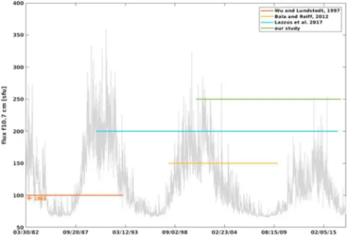
Figure 1 shows the temporal coverage of the database used in this study, compared to previous studies. The temporal coverage of our study is represented by the green line. As GPS ns41 data start at 00:00 14 January 2001, we consider a set of 134,398 hourly data of solar wind parameters, geomagnetic Dst index, and GPS data between this starting date and 23:00 31 December 2016. This includes 49 storm times, listed in Table 1. Part of those storm times were included in the list used in Ji et al. (2012) and Chandorkar et al. (2017).
Studies done in the past to predict the geomagnetic index Dst have shown that various solar wind para-meters are of interest to optimize the performance of predicting models. In the present study, we focused on the use of the densityn, the velocityV, the IMF|B|, and itsBzcomponent. Concerning parameters provided by the GPS ns41, we use the magneticfield measured by the GPS, BsatGPS.
3. Computational Method
3.1. Description of the LSTM NN
The LSTM NN belongs to the family of recurrent neural network (RNN). In a RNN, hidden layers are built to allow information persistence. They behave as a loop to allow information to be passed from one cell of the network to the next. When this loop is unrolled, the RNN can then be thought as multiple copies of the same network. This specific architecture is thought to be very efficient in forecasting time series. Hochreiter (1991) and Bengio et al. (1994) underlined a weakness of RNN. They are supposed to connect past information to the present, but if the information needed is too far in the past, RNN are unable to learn how to connect the information. This failure is due to the vanishing gradient problem occurring during the training phase of RNN.
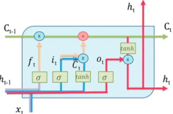
LSTM are designed to avoid this problem. They are made to remember information for long periods of time. They have a chain-like structure like RNN, but the repeating module has a specific structure. Figure 2 repre-sents a LSTM cell. Two elements are fundamental in this cell: the cell state and gates. The cell state in green on Figure 2 is like a conveyor belt, which is connected to gates. Gates can add or remove information from the Figure 1.Temporal coverage of database used in this study and in previous
studies. Wu and Lundstedt (1997) is in orange and their database starts in 1963, Bala and Reiff (2012) is in yellow, Lazzús et al. (2017) is in blue, and our study is in green. The f10.7 in grey represents the variation of solar activity.
cell state depending on information required by the cell. Basically, three gates are used: an input gate in blue, a forget gate in purple, and an output gate in red on Figure 2.
The forget gate can be represented by equation (1).
ft¼σðWfðht1;xtÞ þbfÞ (1)
Table 1
List of Storm Events
Start date Start time End date End time Min. Dst (nT) 19 March 2001 1500 21 March 2001 2300 149 31 March 2001 400 1 April 2001 2100 387 18 April 2001 100 18 April 2001 1300 114 22 April 2001 200 23 April 2001 1500 102 17 August 2001 1600 18 August 2001 1600 105 30 September 2001 2300 2 October 2001 0 148 21 October 2001 1700 24 October 2001 1100 187 28 October 2001 300 29 October 2001 2200 157 23 March 2002 1400 25 March 2002 500 100 17 April 2002 1100 19 April 2002 200 127 19 April 2002 900 21 April 2002 600 149 11 May 2002 1000 12 May 2002 1600 110 23 May 2002 1200 24 May 2002 2300 109 1 August 2002 2300 2 August 2002 900 102 4 September 2002 100 5 September 2002 0 109 7 September 2002 1400 8 September 2002 2000 181 1 October 2002 600 3 October 2002 800 176 20 November 2002 1600 22 November 2002 600 128 29 May 2003 2000 30 May 2003 1000 144 17 June 2003 1900 19 June 2003 300 141 11 July 2003 1500 12 July 2003 1600 105 17 August 2003 1800 19 August 2003 1100 148 20 November 2003 1200 22 November 2003 0 422 22 January 2004 300 24 January 2004 0 149 11 February 2004 1000 12 February 2004 0 105 3 April 2004 1400 4 April 2004 800 112 22 July 2004 2000 23 July 2004 2000 101 24 July 2004 2100 26 July 2004 1700 148 26 July 2004 2200 30 July 2004 500 197 30 August 2004 500 31 August 2004 2100 126 11 November 2004 2200 13 November 2004 1300 109 21 January 2005 1800 23 January 2005 500 105 7 May 2005 2000 9 May 2005 1000 127 29 May 2005 2200 31 May 2005 800 138 12 June 2005 1700 13 June 2005 1900 106 31 August 2005 1200 1 September 2005 1200 131 13 April 2006 2000 14 April 2006 2300 111 14 December 2006 2100 16 December 2006 300 147 26 September 2011 1400 27 September 2011 1200 101 24 October 2011 2000 25 October 2011 1400 132 8 March 2012 1200 10 March 2012 1600 131 23 April 2012 1100 24 April 2012 1300 108 15 July 2012 100 16 July 2012 2300 127 30 September 2012 1300 1 October 2012 1800 119 8 October 2012 200 9 October 2012 1700 105 13 November 2012 1800 14 November 2012 1800 108 17 March 2013 700 18 March 2013 1000 132 31 May 2013 1800 1 June 2013 2000 119 18 February 2014 1500 19 February 2014 1600 112
withσa sigmoid function andWfandbf, respectively, the weight and bias of this layer. This notation is kept for subsequent equations. This gate compares the information coming from the previous cellht1and the incoming informationxtand outputs forCt1a number between 0 and
1, 0 if the information is rejected, 1 if it is kept.
Then, the input gate layer decides the information that needs to be stored, depending on past information. It behaves like the forget gate as described by equation (2). It is connected to a tanh layer to create a vector of candidate valueseCtfollowing equation (3).
it¼σðWiðht1;xtÞ þbiÞ (2)
withWiandbirespectively, the weight and bias of this layer.
e
Ct¼ tanhðWcðht1;xtÞ þbcÞ (3)
withWcandbc, respectively, the weight and bias of this layer.
We described earlier that the cell state and gates are connected to add or remove information, so the next step consists in the update ofCt1 to obtainCt, the new cell state. This is represented in orange on Figure 2 and by equation (4).
Ct¼ft Ct1þiteCt (4)
Then the last step is done through the output gate detailed by equation (5). First, the sigmoid layer helps to define the output. Second, a tanh multiply the cell state by the output of the sigmoid gate to obtain the required information.
ot¼σðWoðht1;xtÞ þboÞ
ht¼ ot tanh ð ÞCt
(5)
3.2. Training and Optimization of the LSTM
The LSTM NN is trained with a backpropagation algorithm, and thanks to its architecture, the gradient does not tend to vanish. To train a NN, most of the time, the gradient descent optimization algorithm used is the Levenberg-Marquardt (Marquardt, 1963), but here we considered the RMSprop. RMSprop is an unpublished adaptative learning rate method proposed by Geoff Hinton (http://www.cs.toronto.edu/~tij-men/csc321/slides/lecture_slides_lec6.pdf). Parameters like weights and bias of the network are described using the notationθi. We then define with equation (6)gt,ias the gradient of the objective function with respect to the parametersθi. at time stept.
gt;i¼∇θJ θt;i (6)
The update of parameters using RMSprop is described by equation (7). First the running averageE(g2) at time steptis computed, then applied to the compute of parameterθi.
E g2 t;i¼0:9E g 2 t;iþ0:1gt;i2 θtþ1;i ¼ θt;i η E g½ 2 t;iþ∈ gt;i (7)
withηthe learning rate and∈a smoothing term to avoid division by zero. Figure 2.LSTM cell. The cell state is in green, the forget gate in purple, the
To develop the network, the database is divided into three sets: 70% for the training set, 20% for the test set, and 10% for the validation set. To evaluate the NN ability to provide accurate forecast from 1 to 6 hr ahead, we use the root-mean-square error (RMSE) and the correlation coefficient (CC), respectively, defined by equations (8) and (9). RMSE¼ ffiffiffiffiffiffiffiffiffiffiffiffiffiffiffiffiffiffiffiffiffiffiffiffiffiffiffiffiffiffiffiffiffiffiffiffiffiffiffiffiffiffiffiffiffiffiffiffiffiffiffi Xn t¼1 Dstð Þ t Dstb ð Þt 2 =n s (8) CC¼ Cov Dst ;Dstb ffiffiffiffiffiffiffiffiffiffiffiffiffiffiffiffiffiffiffiffiffiffiffiffiffiffiffiffiffiffiffiffiffiffiffiffi Var Dstð ÞVarDstb r (9)
We trained and optimized six LSTM NNs corresponding to forecasts from 1 to 6 hr ahead, using the Lasagne library in Python (http://lasagne.readthedocs.io/en/latest/index.html). This way, we obtained a vector of LSTM functions that we note as NNð Þx , withxbeing input parameters of the model. This function plays a sig-nificant role in the process described in the following section.
3.3. Development of Gaussian Process Applied to Time Series Prediction
A GP can be thought as a generalization of a Gaussian distribution applied to functions. Regression based on GP is a Bayesian method where a prior distribution in function space is conditioned on a given number of observations, giving rise to a posterior distribution. The appeal of using GP is that even though the theoretical formulation might seem rather abstract, dealing with function spaces and probability density applied to func-tions, the practical implementation is rather straightforward, boiling down to a simple analytical expression that requires no more than linear algebra. Moreover, GP regression outputs a Gaussian distribution, which has a natural probabilistic interpretation, rather than a single-point estimate. For a complete description of this method the reader is referred to reference textbooks like Rasmussen and Williams (2006).
A GP can be described by equation (10).
f xð ÞeGPðm xð Þ;k xð ;x0ÞÞ (10)
m xð Þ ¼E f xðð ÞÞ (11)
k xð ;x0Þ ¼Eððf xð Þ m xð ÞÞðf xð Þ 0 m xð Þ0 ÞÞ (12)
A GP is completely specified by its mean functionm(x)described by equation (11) and by its covariance func-tionk(x,x0) described by equation (12). The covariance function specifies how exactly each point influences the values that the other points are likely to take on. The main idea is that ifxiandxjare close by, we expect the output from the functions at these points to be similar. Different types of covariance functions exist, also called kernels, which determine the form of the model. Chandorkar and Camporeale (2018) listed common kernels used in machine learning and described how the choice of it is fundamental. In this study, we focused on the NN kernel described by equation (13) (Williams & Barber, 1998).
KNNðx;x0Þ ¼ 2 π 2xTx0 ffiffiffiffiffiffiffiffiffiffiffiffiffiffiffiffiffiffiffiffiffiffi 1þ2xTx ð Þ p ffiffiffiffiffiffiffiffiffiffiffiffiffiffiffiffiffiffiffiffiffiffiffiffiffi 1þ2x0Tx0 q 0 B @ 1 C A (13)
As Rasmussen and Williams (2006) described, if there is no prior knowledge about the function to be approxi-mated, the mean function is defined to be zero. The aim of our study here is to combine the NN performance and the GP process to obtain accurate forecast with an uncertainty distribution. Hence, the mean function m(x) is provided by the NNð Þx function described in section 3.2.
The joint distribution of the training output fand the test outputs f* according to the prior, is given by equation (14). f f ¼ℵ m xð Þ m xð Þ ; K Xð ;XÞ K Xð ;XÞ K Xð ;XÞ K Xð ;XÞ (14)
If there arentraining andn*test points, thenK(X,X*) represents then×n*matrix of the covariance of all
pairs of training and test points.
To make predictions, the posterior distribution over function is needed. To get the posterior distribution, we need to restrict the prior distribution from equation (14) only to those functions thatfit the observed data points. It needs to be conditioned on the observations as described by the system of equation (15).
fjX;X;f ∼N f;covð Þf
f¼m xð Þ þ K Xð ;XÞ½K Xð ;XoÞ1ðym xð ÞÞ covð Þ ¼f K Xð ;XÞ K Xð ;XÞ½K Xð ;XÞ1K Xð ;XÞ
(15)
With this system of equation, test set function valuesf*can now be sampled from the joint posterior
distribu-tion by evaluating the mean and covariance matrix.
To predict the geomagnetic index Dst based on input featuresx, the equation (16) summarizes the inher-ent process. DstðtþpÞ ¼f xð t1Þ þ∈ ∈ ∼Nð0;σ2Þ f xtþp ∼GP NNxtþp ;KNN xtþp;xsþp (16)
withpbeing the expected time forecast. Here we consider p= {1,2,3,4,5,6} to provide multistep ahead prediction of the Dst index from 1 to 6 hr ahead. The GP part is developed using the Matlab Software GPML, available at http://www.gaussianprocess.org/gpml/code (Rasmussen & Nickisch, 2010).
4. Results
4.1. Optimization of the LSTM NN
Thefirst step in the development of the GPNN model is to optimize the performance of each LSTM to provide predictions of Dst from 1 to 6 hr ahead. To train LSTM, we use solar wind data and GPS data described in section 2 (the densityn, the velocityV, the IMF∣B∣, itsBzcomponent, and the magneticfield measured by the GPS ns41,BsatGPS). We also use the past history of Dst, from 1 to 6 hr back. This is summarized with
the equation (17).
b
DstðtþpÞNN¼NNðn tð Þ;V tð Þ;IMFj jBð Þt ;Bz tð Þ;BsatGPSð Þt ;
Dstðt1 hrÞ;Dstðt2 hrÞ; …;Dstðt6 hrÞÞ
(17)
Tofind the LSTM structure, which is the most suitable for predicting geomagnetic storms, we train it using various numbers of cells. The optimal number is 20 and after training, testing, and validating each LSTM, we compare their performance to NN models proposed in the past to predict Dst. Figure 3 presents a com-parison of CC and RMSE between our model, with and without using GPS data, and previous models predict-ing Dst based on NN. The temporal coverage of these previous studies is shown in Figure 1 so the reader can have an estimation of the storm times used in them.
The persistence is also presented. It uses the previous value of Dst as the prediction for the next step Dst = Dst(t1). This is a simple model, which can be used as a baseline and provide great performance for short-term forecast because of the high correlation between Dst values within 1 hr.
Our models, with or without GPS data, provides performance, which are close to the one obtained by Lazzús et al. (2017) from 1 to 3 hr ahead but when the expected forecast goes from 4 to 6 hr ahead, our models, with
or without GPS data, provide better global performance. As an example, when considering a 6-hr-ahead forecast, our model with GPS data provides a CC of 0.873 and a RMSE of 9.86, while Lazzús et al. (2017) obtained a CC of 0.826 and a RMSE of 13.09. As the Lazzús et al. (2017) model is based only on previous Dst values, it shows the benefit of using exogenous data when predicting a geomagnetic index. Bala and Reiff (2012) used the Boyle index as an input function, and obtained quite similar performance as ours. If we consider again a forecast of 6 hr ahead, their model presents a CC of 0.77 and a RMSE of 11.09. It is slightly worse than our model with or without GPS data. We also decided to compare our model with the one provided by Wu and Lundstedt (1997) as it is thefirst model using recurrent network. We wanted to compare the performance of a classic recurrent network to the LSTM, and see how the complexity of the LSTM cell could provide more accurate predictions. Wu and Lundstedt (1997) provided for a 6-hr-ahead Figure 3.LSTM performance in comparison to previous models. Our model with and without GPS data is highlighted in blue.
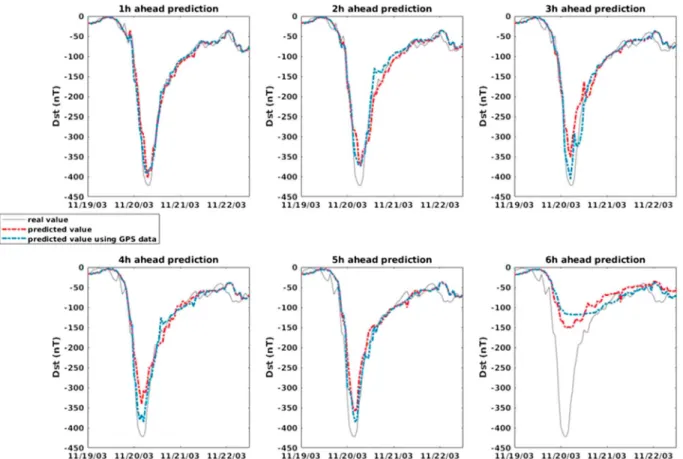
forecast a CC of 0.82 and a RMSE of 20.8, showing in comparison to our model with or without GPS data, that the LSTM cell brings more accuracy. We observed that using GPS data generally results in an improvement when considering important geomagnetic storms. Figure 4 presents predictions obtained with the LSTM NN, with GPS data in blue and without GPS data in red, for Dst forecast from 1 to 6 hr ahead, for the 2003 Halloween storm event (peak at422 nT). Predictions for 1 to 2 hr ahead are very similar, but when we consider the forecast of 3 hr ahead, the model without GPS data predicts a peak of348 nT while the model with the GPS data provides a prediction of405 nT. For a forecast done 4 hr ahead, the model without GPS data provides a prediction of335 nT and the one with GPS data, a forecast of380 nT. For predictions done 5 hr ahead, predicted peak values are quite the same. However, the 6-hr-ahead forecast shows that a single-point prediction provided by the NN is not good enough and offers a strong rationale to combine the NN performance with the GP model to obtain a probabilistic forecast.
4.2. Evaluation of the GPNN Process
As we described before, the GP process aim to provide not only a single point prediction but also an asso-ciated uncertainty. Metrics like RMSE and CC are defined for single-point prediction and are not adequate to evaluate probabilistic forecast.
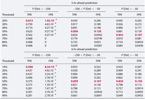
Storm activity is often classified using given thresholds of Dst values. According to the most common classification, we distinguished three levels of storms summarized in Table 2 (Dst<250,250≤Dst<50, Dst≥50). The aim here is to use metrics, which will be able to evaluate how the GPNN manages to forecast geomagnetic storms into the right “family”of storm. To do so, we focused on the receiver operating charac-teristic (ROC) curve and reliability diagram.
Figure 4.LSTM predictions without GPS data (in red dot line) and with GPS data (in blue dot line) for the 2003 Halloween storm. The real value is the grey line.
Table 2
Storm Classification
Level of activity Storm classification Dst>50 nT Moderate
250 nT<Dst<50 nT Intense Dst<250 nT Super storm
Table 3
False and True Positive Ratios for Each Storm Category
1-hr-ahead prediction P(Dst)<250 250<P(Dst)<50 P(Dst)>50 Threshold TPR FPR TPR FPR TPR FPR 10% 0.969 2.70.103 0.981 0.163 0.999 0.434 20% 0.969 1.11.103 0.961 0.105 0.996 0.321 30% 0.969 6.40.104 0.927 0.0719 0.991 0.240 40% 0.969 4.00.104 0.895 0.049 0.984 0.185 50% 0.844 3.00.104 0.855 0.0270 0.972 0.138 60% 0.812 2.78.104 0.806 0.0161 0.951 0.102 70% 0.656 2.78.104 0.753 9.30.103 0.929 0.0705 80% 0.625 2.78.104 0.670 3.95.103 0.895 0.0371 90% 0.468 9.27.105 0.554 1.61.103 0.838 0.0178 2-hr-ahead prediction P(Dst)<250 250<P(Dst)<50 P(Dst)>50 Threshold TPR FPR TPR FPR TPR FPR 10% 0.969 3.15.103 0.963 0.199 0.999 0.388 20% 0.937 9.27.104 0.934 0.142 0.984 0.273 30% 0.937 3.71.104 0.914 0.105 0.973 0.211 40% 0.906 1.85.104 0.891 0.0834 0.961 0.167 50% 0.781 1.85.104 0.863 0.0565 0.943 0.134 60% 0.6875 9.27.105 0.824 0.0390 0.917 0.107 70% 0.656 9.27.105 0.783 0.0268 0.895 0.0845 80% 0.500 9.27.105 0.720 0.0156 0.858 0.0646 90% 0. .437 0 0.601 5.68103 0.802 0.0363 3-hr-ahead prediction P(Dst)<250 250<P(Dst)<50 P(Dst)>50 Threshold TPR FPR TPR FPR TPR FPR 10% 0.875 3.24.103 0.958 0.254 0.984 0.373 20% 0.843 9.27.104 0.939 0.186 0.971 0.278 30% 0.813 4.64.104 0.912 0.139 0.955 0.228 40% 0.750 1.86.104 0.890 0.106 0.940 0.182 50% 0.625 9.27.105 0.880 0.0819 0.919 0.146 60% 0.593 0 0.809 0.0606 0.893 0.1058 70% 0.593 0 0.766 0.0451 0.826 0.0865 80% 0.437 0 0.714 0.0291 0.814 0.0594 90% 0.406 0 0.614 0.0164 0.747 0.0413 4-hr-ahead prediction P(Dst)<250 250<P(Dst)<50 P(Dst)>50 Threshold TPR FPR TPR FPR TPR FPR 10% 0.906 3.24.103 0.968 0.311 0.970 0.339 20% 0.875 1.29.103 0.953 0.252 0.949 0.243 30% 0.813 7.42.104 0.933 0.208 0.931 0.192 40% 0.813 6.49.104 0.916 0.169 0.906 0.144 50% 0.781 9.27.105 0.895 0.138 0.874 0.104 60% 0.687 9.27.105 0.843 0.106 0.841 0.0803 70% 0.562 9.27.105 0.795 0.0812 0.802 0.0636 80% 0.468 9.27.105 0.742 0.0621 0.76 0.0449 90% 0.437 9.27.105 0.640 0.0403 0.699 0.0300 5-hr-ahead prediction P(Dst)<250 250<P(Dst)<50 P(Dst)>50 Threshold TPR FPR TPR FPR TPR FPR 10% 0.812 3.06.103 0.956 0.316 0.962 0.346
4.2.1. Receiver Operating Characteristic Curve
Our GPNN model provides to an operator a probabilistic forecast, which can be used in a decision-making scenario. For example, a decision made by an operator to turnoff a system according to the level of storm might be taken when the forecast probability of this storm exceeds a predetermined“trigger”threshold. For any storm, a graph called receiver operating characteristic curve (know as ROC curve) can be constructed. This ROC curve is based on a contingency table in which predictions of Dst are classified according to the real value of Dst. The aim is to estimate the probability of a prediction to belong to the right category of storm via binary classification, in the sense“one category versus all the others.”Camporeale et al. (2017) used the same process to classify the category of solar events between ejecta, coronal hole, sector reversal, and streamer belt. The ROC curves represent the false positive ratio (FPR) versus the true positive ratio (TPR). The FPR is the ratio of false positive divided by the total number of negatives. The TPR also called sensitivity is the ratio of true positives divided by the total number of positives. For perfect classifications, the FPR has to be equal to 0 and TPR equal to 1; thus, the value of the threshold that produces the point closest to these values is optimal.
Table 3 presents ROC values obtained from 1- to 6-hr-ahead forecasts, depending on the level of storm. The ROC is usually shown graphically, but numerical values are more relevant for the reader to analyze variations depending on the threshold. The optimal threshold is in red and bold; it is computed to minimize the Euclidean distance from FPR = 0 and TPR = 1. ROC values obtained for the highest level of activity, meaning Dst values<250 nT provide FPR for each threshold (the highest value is 2.7.103for a 10% threshold when considering a 1-hr forecast). The TPR behavior is more complicated to generalize. For predictions done from 1 to 5 hr ahead, values are always greater than 0.719 for thresholds from 10% to 40%, and then there is a decrease. If we focus on the 6-hr-ahead forecast, the best TPR is 0.5 for a 10% threshold. It means that the more there is an increasing probability for a superstorm to occur, the less the model is able to forecast it with-out misjudgments 6 hr in advance. However, for intense storms (250 nT<Dst<50 nT), the GPNN pro-vides TPR higher than 0.670 for thresholds between 10% and 80%, and for moderate storms, this model provides TPR higher than 0.649 for every thresholds, from 1 to 6 hr ahead.
Table 3(continued) 5-hr-ahead prediction P(Dst)<250 250<P(Dst)<50 P(Dst)>50 Threshold TPR FPR TPR FPR TPR FPR 20% 0.812 1.02.103 0.934 0.246 0.945 0.265 30% 0.750 4.63.104 0.917 0.189 0.926 0.215 40% 0.719 9.27.105 0.891 0.148 0.906 0.171 50% 0.625 9.27.105 0.856 0.120 0.881 0.139 60% 0.562 9.27.105 0.824 0.0942 0.853 0.107 70% 0.468 0 0.779 0.0740 0.810 0.081 80% 0.468 0 0.725 0.055 0.754 0.0654 90% 0.468 0 0.639 0.0381 0.685 0.0430 6-hr-ahead prediction P(Dst)<250 250<P(Dst)<50 P(Dst)>50 Threshold TPR FPR TPR FPR TPR FPR 10% 0.500 8.34.103 0.953 0.352 0.932 0.307 20% 0.437 4.92.103 0.928 0.289 0.909 0.241 30% 0.437 3.24.103 0.904 0.244 0.886 0.186 40% 0.406 2.78.103 0.890 0.202 0.862 0.161 50% 0.375 1.76.103 0.859 0.167 0.834 0.130 60% 0.375 1.39.103 0.821 0.138 0.798 0.113 70% 0.281 7.47.104 0.788 0.115 0.757 0.0914 80% 0.281 3.70.104 0.735 0.0926 0.712 0.0693 90% 0.281 2.78.104 0.661 0.0691 0.649 0.0455
4.2.2. Reliability Diagram
The ROC discussed in the previous section gives information about the ability of the forecast system to detect the occurrence of a geomagnetic storm event for a given threshold, in terms of false and true positive. Reliability diagrams measure how closely the forecast probabilities of an event correspond to the actual fre-quency with which an event is observed. A perfectly reliable forecast is one in which an event predicted with probabilitypis observed, on average, with frequencyp. The reliability diagram bins the forecasts into groups according to the issued probability, shown on the horizontal axis. The frequency with which an event was observed to occur for each bin is then plotted on the vertical axis. If the reliability curve lies above/below the perfect diagonal slope, the resulting forecasts are under/over confident, that is, they yield smaller/higher probabilities for a specific outcome than observed.
Figure 5 presents reliability diagrams obtained from 1- to 6-hr-ahead forecasts. It shows that the 1-hr-ahead forecast slightly underestimates the storm, when there are more than 35% of probabilities for a given value of Dst. For example, when there is 80% of risk for a predicted storm, the real observed frequency of it is 90%. The GPNN provides reliable forecast for 2-hr-ahead prediction, as the observed frequency of storm regarding the predicted probability defines almost perfectly a diagonal. For predictions further than 3 hr ahead, the more it goes in time, the more it overestimates the probability of storms. If we focus on the 6-hr-ahead prediction, when the GPNN model provides a predicted probability of 90%, the real observed frequency is of 65%. This model is overconfident. Once the reliability diagram is obtained, it is of interest to seek simple correc-tions to the forecast probabilities (re-calibration). This issue will be investigated elsewhere in greater detail. Here we just show Figure 6 that by multiplying the standard deviation by a factor of 2 or 3, it is possible to improve the reliability for predicted probability higher than 50% (Figure 6). For example, if the predicted probability is 90%, by multiplying sigma by 2, the corresponding real frequency is 72% and if we multiply by 3, we get 80%. This way, we managed to get closer to the diagonal, when the probability of events increases. Conversely, a simple rescaling of the obtained standard deviation yields worse reliability for prob-abilities smaller than 50%.
Figure 7 presents predictions provided by the GPNN model for the 2003 Halloween storm. For predictions from 1 to 5 hr ahead, thanks to this process, the predicted value of Dst is close to the real value. For example, for 5 hr ahead, the real peak of activity of422 nT has a predicted value of391 nT. The main contribution of the GP process here is shown for the 6-hr-ahead forecast. While the LSTM alone failed to reach the highest Figure 5.Reliability diagram for Dst forecast from 1 to 6 hr ahead. The diagonal is in red dot line.
peak of activity, the GPNN manages to have a predicted value closer to the real value than the LSTM one, and the covariance over the mean value encompasses the peak of activity (compare with Figure 4).
5. Conclusion
In this paper, we have presented a model to predict the geomagnetic index Dst from 1 to 6 hr ahead, based on the combination of ANN and GP, called GPNN.
First, we developed a LSTM NN to provide Dst predictions from 1 to 6 hr ahead. A specific LSTM has been developed for each time predictions, then global performance of LSTM has been compared to past forecast-ing models of Dst. It shows that the LSTM provides very good global performance in comparison to previous models. When focusing on superstorm like the well-known 2003 Halloween storm, we underlined that even if global metrics are excellent, the 6-hr-ahead forecast fails to predict the highest peak of activity.
Second, to obtain a probabilistic forecast instead of a single point prediction, we developed a GP, which con-siders the LSTM as the mean function. Thanks to this combination, we observed that we managed to predict accurately superstorm like the 2003 Halloween storm for predictions from 1 to 5 hr ahead. For the 6-hr-ahead prediction, the covariance manages to encompass the peak of activity.
To evaluate this probabilistic forecast, we use ROC curves and reliability diagram. ROC curves demonstrate that for each time forecast, storm level, and threshold, the FPR is very low. However, concerning TPR, values are great for moderate and intense storms, but for 6-h-ahead prediction of superstorm, misjudgment is pos-sible when the threshold increases. In this case, the optimal threshold is around 10%, which will need further improvement. The reliability diagram shows that as the prediction goes further in time, the GPNN provides great performance for predictions from 1 to 3 hr ahead, but for 4 to 6 hr ahead, an overestimation of the Figure 7.GPNN performance to predict Dst for the 2003 Halloween storm. The predicted value is the purple dot line. The real value is the deep blue line. The gray shadow represents one standard deviation.
storm is possible. We also demonstrate that, thanks to this diagram, it is possible to evaluate the optimization required to improve the reliability of the GPNN, and possibly to re-calibrate the prediction.
References
Akasofu, S. I. (1981). Energy coupling between the solar wind and the magnetosphere.Space Science Reviews,28(2), 121–190. https://doi.org/ 10.1007/BF00218810
Astafyeva, E. (2009). Effects of strong IMF Bz southward events on the equatorial and mid-latitude ionosphere.Annales Geophysicae,27(3), 1175–1187.
Ayala Solares, J. R., Wei, H. L., Boynton, R. J., Walker, S. N., & Billings, S. A. (2016). Modeling and prediction of global magnetic disturbance in near-Earth space: A case study for Kp index using NARX models.Space Weather,14, 899–916. https://doi.org/10.1002/
2016SW001463
Bala, R., & Reiff, P. (2012). Improvements in short-term forecasting of geomagnetic activity.Space Weather,10, S06001. https://doi.org/ 10.1029/2012SW000779
Balikhin, M. A., Boynton, R. J., Walker, S. N., Borovsky, J. E., Billings, S. A., & Wei, H. L. (2011). Using the NARMAX approach to model the evolution of energetic electronsfluxes at geostationary orbit.Geophysical Research Letters,38, L18105. https://doi.org/10.1029/ 2011GL048980
Bengio, Y., Simard, P., & Frasconi, P. (1994). Learning long-term dependencies with gradient descent is difficult.IEEE Transactions on Neural Networks,5(2), 157–166. https://doi.org/10.1109/72.279181
Boynton, R. J., Balikhin, M. A., Billings, S. A., Wei, H. L., & Ganushkina, N. (2011). Using the NARMAX OLS-ERR algorithm to obtain the most influential coupling functions that affect the evolution of the magnetosphere.Journal of Geophysical Research,116, A05218. https://doi. org/10.1029/2010JA015505
Burton, R. K., McPherron, R. L., & Russell, C. T. (1975). An empirical relationship between interplanetary conditions and Dst.Journal of Geophysical Research,80, 4204–4214. https://doi.org/10.1029/JA080i031p04204
Camporeale, E., Carè, A., & Borovsky, J. E. (2017). Classification of solar wind with machine learning.Journal of Geophysical Research: Space Physics,122, 10,910–10,920. https://doi.org/10.1002/2017JA024383
Chandorkar, M., & Camporeale, E. (2018). Probabilistic Forecasting of Geomagnetic Indices Using Gaussian Process Models. InMachine Learning Techniques for Space Weather(pp. 237–258).
Chandorkar, M., Camporeale, E., & Wing, S. (2017). Probabilistic forecasting of the disturbance storm time index: An autoregressive Gaussian process approach.Space Weather,15, 1004–1019. https://doi.org/10.1002/2017SW001627
Elman, J. L. (1990). Finding structure in time.Cognitive Science,14(2), 179–211. https://doi.org/10.1207/s15516709cog1402_1 Gleisner, H., Lundstedt, H., & Wintoft, P. (1996). Predicting geomagnetic storms from solar-wind data using time-delay neural networks.
Annales de Geophysique,14(7), 679–686. https://doi.org/10.1007/s00585-996-0679-1
Gonzalez, W. D., Joselyn, J. A., Kamide, Y., Kroehl, H. W., Rostoker, G., Tsurutani, B. T., & Vasyliunas, V. M. (1994). What is a geomagnetic storm?
Journal of Geophysical Research,99(A4), 5771–5792. https://doi.org/10.1029/93JA02867
Haykin, S. (1998).Neural networks: A comprehensive foundation. Upper Saddle River, N. J: Prentice Hall.
Hochreiter, S. (1991). Untersuchungen zu dynamischen neuronalen Netzen.Diploma, Technische Universität München,91, 1. Hochreiter, S., & Schmidhuber, J. (1997). Long short-term memory.Neural Computation,9(8), 1735–1780. https://doi.org/10.1162/neco.
1997.9.8.1735
Iyemori, T., Maeda, H., & Kamei, T. (1979). Impulse response of geomagnetic indices to interplanetary magneticfields.Journal of Geomagnetism and Geoelectricity,31(1), 1–9. https://doi.org/10.5636/jgg. 31.1
Ji, E. Y., Moon, Y. J., Gopalswamy, N., & Lee, D. H. (2012). Comparison of Dst forecast models for intense geomagnetic storms.Journal of Geophysical Research,117, A03209. https://doi.org/10.1029/2011JA016872
Kennedy, J., & Eberhart, R. (1995). Particle swarm optimization. InProceedings of the IEEE International Conference on Neural Networks
(pp. 1942–1948). Piscataway, N. J.: IEEE Press. https://doi.org/10.1109/ICNN.1995.488968
Lazzús, J. A., Vega, P., Rojas, P., & Salfate, I. (2017). Forecasting the Dst index using a swarm-optimized neural network.Space Weather,15, 1068–1089. https://doi.org/10.1002/2017SW001608
Lundstedt, H., Gleisner, H., & Wintoft, P. (2002). Operational forecasts of the geomagnetic Dst index.Geophysical Research Letters,29(24), 2181. https://doi.org/10.1029/2002GL016151
Lundstedt, H., & Wintoft, P. (1994). Prediction of geomagnetic storms from solar wind data with the use of a neural network.Annales de Geophysique,12(1), 19–24. https://doi.org/10.1007/s00585-994-0019-2
Marquardt, D. W. (1963). An algorithm for least-squares estimation of nonlinear parameters, 871.Journal of the Society for Industrial and Applied Mathematics,11(2), 431–441.
Morley, S. K., Sullivan, J. P., Carver, M. R., Kippen, R. M., Friedel, R. H. W., Reeves, G. D., & Henderson, M. G. (2017). Energetic particle data from the global positioning system constellation.Space Weather,15, 283–289. https://doi.org/10.1002/2017SW001604
Rasmussen, C. E., & Nickisch, H. (2010). Gaussian processes for machine learning (GPML) toolbox.Journal of Machine Learning Research,
11(Nov), 3011–3015.
Rasmussen, C. E., & Williams, C. K. (2006).Gaussian processes for machine learning(Vol. 38, pp. 715–719). Cambridge, MA, USA: The MIT Press. Rastätter, L., Kuznetsova, M. M., Glocer, A., Welling, D., Meng, X., Raeder, J., et al. (2013). Geospace environment modeling 2008-2009
challenge: Dst index.Space Weather,11, 187–205. https://doi.org/10.1002/swe. 20036
Rumelhart, D. E., & McClelland, J. (1986).Parallel distributed processing: Explorations in the microstructure of cognition. Cambridge, Mass: MIT Press.
Singh, A. K., Siingh, D., & Singh, R. P. (2010). Space weather: Physics, effects and predictability.Surveys in Geophysics,31(6), 581–638. https:// doi.org/10.1007/s10712-010-9103-1
Sugiura, M. (1964). Hourly values of equatorial Dst for the IGY.Annals of the International Geophysical Year,35, 9–45. Waibel, A., Hanazawa, T., Hinton, G., Shikano, K., & Lang, K. J. (1989). Phoneme recognition using time-delay neural networks.
IEEE Transactions on Acoustics, Speech, and Signal Processing,37(3), 328–339. https://doi.org/10.1109/29.21701
Wei, H. L., Billings, S. A., Sharma, A. S., Wing, S., Boynton, R. J., & Walker, S. N. (2011). Forecasting relativistic electronflux using dynamic multiple regression models.Annales Geophysicae,29(2), 415–420. https://doi.org/10.5194/angeo-29-415-2011
Williams, C. K., & Barber, D. K. (1998). Bayesian classification with Gaussian processes.IEEE Transactions on Pattern Analysis and Machine Intelligence,20(12), 1342–1351. https://doi.org/10.1109/34.735807
Acknowledgments
This project has been supported by a CWI internship grant. E. C. was partially funded by the NWO-Vidi grant 639.072.716. Authors would like to thank the CXD team at Los Alamos National Laboratory for providing GPS data. The solar wind plasma data of OMNI were obtained from the National Space Science Data Center (NSSDC) of National Aeronautics and Space Administration (NASA) (https:// omniweb.gsfc.nasa.gov/ow.html). This research activity is also supported by the Centre National d’Etudes Spatiales (CNES) under the supervision of Denis Standarovki and the Office National d’Etudes et de Recherches Aérospatiales (ONERA). The code will be made available after publication on our website www.mlspaceweather.org.
Wing, S., Johnson, J. R., Jen, J., Meng, C. I., Sibeck, D. G., Bechtold, K., & Takahashi, K. (2005). Kp forecast models.Journal of Geophysical Research,110, A04203. https://doi.org/10.1029/2004JA010500
Wu, J.-G., & Lundstedt, H. (1997). Geomagnetic storm predictions from solar wind data with the use of dynamic neural networks.Journal of Geophysical Research,102, 14,255–14,268. https://doi.org/10.1029/97JA00975