A Dissertation by
ANIRBAN MONDAL
Submitted to the Office of Graduate Studies of Texas A&M University
in partial fulfillment of the requirements for the degree of DOCTOR OF PHILOSOPHY
August 2011
A Dissertation by
ANIRBAN MONDAL
Submitted to the Office of Graduate Studies of Texas A&M University
in partial fulfillment of the requirements for the degree of DOCTOR OF PHILOSOPHY
Approved by:
Co-Chairs of Committee, Bani K. Mallick Yalchin Efendiev Committee Members, Faming Liang
Akhil Datta-Gupta Samiran Sinha Head of Department, Simon J. Sheather
August 2011 Major Subject: Statistics
ABSTRACT
Bayesian Uncertainty Quantification for Large Scale Spatial Inverse Problems. (August 2011)
Anirban Mondal, B.S., University of Calcutta; M.Stat., Indian Statistical Institute;
M.S., Michigan State University
Co–Chairs of Advisory Committee: Dr. Bani K. Mallick Dr. Yalchin Efendiev
We considered a Bayesian approach to nonlinear inverse problems in which the un-known quantity is a high dimension spatial field. The Bayesian approach contains a natural mechanism for regularization in the form of prior information, can incorpo-rate information from heterogeneous sources and provides a quantitative assessment of uncertainty in the inverse solution. The Bayesian setting casts the inverse solution as a posterior probability distribution over the model parameters. Karhunen-Lo´eve expansion and Discrete Cosine transform were used for dimension reduction of the random spatial field. Furthermore, we used a hierarchical Bayes model to inject multiscale data in the modeling framework. In this Bayesian framework, we have shown that this inverse problem is well-posed by proving that the posterior measure is Lipschitz continuous with respect to the data in total variation norm. The need for multiple evaluations of the forward model on a high dimension spatial field (e.g. in the context of MCMC) together with the high dimensionality of the posterior, results in many computation challenges. We developed two-stage reversible jump MCMC method which has the ability to screen the bad proposals in the first inex-pensive stage. Channelized spatial fields were represented by facies boundaries and variogram-based spatial fields within each facies. Using level-set based approach, the
shape of the channel boundaries was updated with dynamic data using a Bayesian hierarchical model where the number of points representing the channel boundaries is assumed to be unknown. Statistical emulators on a large scale spatial field were introduced to avoid the expensive likelihood calculation, which contains the forward simulator, at each iteration of the MCMC step. To build the emulator, the original spatial field was represented by a low dimensional parameterization using Discrete Cosine Transform (DCT), then the Bayesian approach to multivariate adaptive re-gression spline (BMARS) was used to emulate the simulator. Various numerical results were presented by analyzing simulated as well as real data.
ACKNOWLEDGMENTS
I would like to express my deepest gratitude to my co-advisors Prof. Bani K. Mallick and Prof. Yalchin Efendiev. Without their guidance and persistent help this disserta-tion would not have been possible. I would like to thank my PhD committee members, Prof. Akhil Datta-Gupta, Prof. Faming Liang and Dr. Samiran Sinha for their help and support. A special thanks goes to Prof. Michael Longnecker for bailing me out of difficulties with his invaluable advice and constant support. A big thanks goes to my friends and peers for the enjoyable time we spent together at Texas A&M and Michigan State University. Last, but not least, I express my profound appreciation to Paromita for her encouragement, understanding, love and support during the hard times of this study. The research work discussed in this dissertation is supported in parts by Research Grant NSF CMG 0724704 and by Award Number KUS-C1-016-04 made by King Abdullah University of Science and Technology (KAUST).
TABLE OF CONTENTS
Page
ABSTRACT . . . iii
DEDICATION . . . v
ACKNOWLEDGMENTS . . . vi
TABLE OF CONTENTS . . . vii
LIST OF TABLES . . . x
LIST OF FIGURES . . . xi
CHAPTER I INTRODUCTION. . . 1
I.1. Different Examples of the Inverse Problem . . . 2
I.1.1. Reservoir Characterization . . . 2
I.1.2. Ground Water Flow . . . 4
I.1.3. Weather Forecasting . . . 5
II MULTISCALE DATA INTEGRATION IN LARGE-SCALE SPATIAL INVERSE PROBLEMS . . . 9
II.1. Bayesian Framework . . . 12
II.1.1. Modeling the Prior Process P(Y) . . . 13
II.1.2. Modeling the Fine Scale DataP(yo|Y) . . . 15
II.1.3. Modeling P(yc|Y, yo) by Upscaling . . . 16
II.1.4. Modeling the Likelihood P(d|Y, yc, yo) . . . 17
II.1.5. Prior Distributions . . . 18
II.1.6. The Posterior Distribution and its Continuity . . 18
II.2. Bayesian Computation Using MCMC . . . 20
II.3. Extension to Model with Unknownm . . . 23
II.5. Simulated and Real Examples from Reservoir Model . . . 27
II.5.1. The Mathematical Model and Specification of G. . . 29
II.5.2. The Upscaling Procedure . . . 31
II.5.3. Numerical Results for Simulated Reservoirs . . . 33
II.5.4. Numerical Results for a Real Field Example . . 34
II.6. Conclusions . . . 39
III INVERSE PROBLEMS IN SPATIAL FIELDS WITH CHAN-NELIZED STRUCTURE . . . 43
III.1. Parameterization of the Channelized Spatial Field . . . . 48
III.2. Bayesian Hierarchical Model . . . 50
III.2.1. Modeling the Likelihood P(z|k) . . . 51
III.2.2. Modeling the Prior Process P(k) . . . 51
III.3. Posterior Error Introduced by Truncation . . . 52
III.4. Reversible Jump MCMC . . . 54
III.4.1. An Example . . . 57
III.5. Two-stage Reversible Jump MCMC . . . 61
III.6. Numerical Results . . . 66
III.7. Conclusions . . . 78
IV EMULATORS ON LARGE SCALE SPATIAL INVERSE PROB-LEMS . . . 81
IV.1. Parametrization of the Spatial Field Using Discrete Cosine Transform (DCT) . . . 87
IV.2. The Bayesian Hierarchical Model . . . 91
IV.2.1. Design of the Simulation Experiments . . . 93
IV.2.2. Modeling the Likelihood Using Bayesian MARS Emulators . . . 94
IV.2.3. Modeling the Coarse Scale Data . . . 97
IV.2.4. Modeling the Observed Fine Scale Data . . . 98
IV.3. Sampling from the Posterior . . . 99
IV.3.1. Hybrid Sampling Algorithm . . . 99
IV.4. Numerical Results . . . 103
IV.4.1. Simulated Reservoir Example . . . 104
IV.5. Conclusion . . . 119
V CONCLUSION AND SUMMARY . . . 120
REFERENCES . . . 123 APPENDIX A . . . 131 APPENDIX B . . . 138 APPENDIX C . . . 139 APPENDIX D . . . 140 VITA . . . 146
LIST OF TABLES
TABLE Page
I Posterior errors when the K-L expansion is truncated toM terms
for two interfaces example.. . . 69 II Posterior errors when the K-L expansion is truncated toM terms
for four interfaces example. . . 77 III Computational times, in seconds, of the emulator based and
LIST OF FIGURES
FIGURE Page
1 The forward simulator. . . 3 2 Flow-chart for the hierarchical model. . . 22 3 Schematic description of fine- and coarse-grids. . . 31 4 Log permeability plot for the simulated example using two stage
reversible jump MCMC. . . 35 5 Histogram of the posterior distribution of m for two-stage
re-versible jump MCMC. . . 35 6 Posterior densities for the simulated example using two-stage
re-versible jump MCMC. . . 36 7 Log permeability plot with only 10 percent fine-scale data
ob-served and no coarse-scale data available. . . 36 8 Posterior densities with only 25 percent fine-scale data observed
and no coarse-scale data available. . . 37 9 Log permeability field using the two stage reversible jump MCMC
for the PUNQ-S3 model. . . 39 10 Posterior density ofl and σ2 for the PUNQ-S3 model. . . . . 40
11 Posterior distributions ofm and θ0 for the PUNQ-S3 model. . . 40
12 Quartiles of the sampled log permeability field for the PUNQ-S3 model. 41 13 Log permeability for the PUNQ-S3 model assuming no coarse
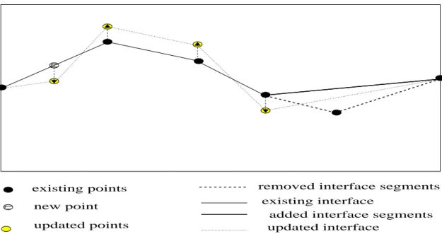
scale data avaialable. . . 41 14 Illustration of the permeability field with facies. . . 48 15 An illustration of the birth, death and jump process in reversible
16 Log permeability field from full reversible jump MCMC. . . 67 17 Fractional flow from full reversible jump MCMC. . . 68 18 Cross-plot between Ek=kFobs−Fkk and Ek∗ =kFobs −Fk∗k. . . 69
19 Log permeability field from two-stage reversible jump MCMC in
three-coarse-block case. . . 71 20 Cross plot and frcational flow from two-stage reversible jump
MCMC in three-coarse-block case. . . 72 21 Fractional flow errors vs. accepted iterations for two-stage and
full reversible jump MCMC. . . 72 22 Cross-plot between Ek=kFobs−Fkk andEk∗ =kFobs−Fk∗kwhen
the variance of the log permeability field is 2. . . 74 23 Log permeability field from two-stage reversible jump MCMC
us-ing mixed MsFEM when the variance of the log permeability field
is 2. . . 75 24 Corss-plot and frcational flow from two-stage reversible jump MCMC
using mixed MsFEM. . . 76 25 Fractional flow errors vs. accepted iterations when the variance
of the log permeability field is 2. . . 76 26 Log permeability field from two-stage reversible jump MCMC
with five coarse blocks. . . 78 27 Comaprison of fractional flow using full reversible jump MCMC
vs two-stage reversible jump MCMC in three-coarse-block case. . . . 79 28 Fractional flow errors vs. accepted iterations for the example with
two channels. . . 79 29 A spatial field, the corresponding DCT coefficients and the spatial
field obtained by the inverse DCT transform. . . 90 30 Cross plot and box plot for the test data. . . 106
31 Fitted mean and 95% credible interval for one set of test data
using the emulator. . . 106 32 Log permeability field for the simulated example using emulator. . . 108 33 Posterior distributions of the model parameters for the simulated
example using emulator. . . 109 34 One dimensional and two dimensional posterior marginals of the
largest DCT coefficients for the simulated model. . . 110 35 Boxplot of the posterior marginals of the DCT coefficients for the
simulated model. . . 111 36 Log permeability field for the PUNQ-S3 model using emulator. . . . 114 37 Posterior distributions of the model parameters for the PUNQ-S3
model using emulator. . . 115 38 One dimensional and two dimensional posterior marginals of the
largest DCT coefficients for the PUNQ-S3 model. . . 116 39 Box plot of the posterior marginals of the DCT coefficients for the
PUNQ-S3 model. . . 117 40 Fitted mean and 95% credible interval of the observed output for
CHAPTER I
INTRODUCTION
Mathematical models are studied using computer simulation in almost all areas of applied and computational mathematics. The indirect estimation of model param-eters or inputs from observations constitutes an inverse problem. Such problems arise frequently in science and engineering, with applications in weather forecast-ing, climate prediction, chemical kinetics and oil reservoir forecasting. Quantifying the uncertainty in inputs or parameters is then essential for predictive modeling and simulation based decision making.
A physical system is often described by a forward model, which predicts some measurable features of the system given a set of model input parameters. The cor-responding inverse problem consists of inferring these input parameters from a set of observations. The simplicity of this definition belies many fundamental challenges. For example, in large scale spatial inverse problems, the observed data may be very limited compared to the dimension of the unknown input spatial field. Moreover, the available observed data may be corrupted by noise and the action of the forward model may include filtering or smoothing effect. These features typically develop ill-posed inverse problems.
Classical statistical approaches have used various regularization methods to im-pose well-im-posedness of the inverse problems. The resulting deterministic problems are solved by optimization and other means; see for example Vogel (2002). Here we focus on the Bayesian approach to nonlinear inverse problems where the input is a high dimension spatial field. As described in Marzouk and Najm (2009), the This dissertation follows the style of the Journal of the Royal Statistical Society.
Bayesian approach contains a natural mechanism for regularization in the form of prior information, can incorporate information from heterogeneous sources and pro-vide a quantitative assessment of uncertainty in the inverse solution (e.g. Kaipio and Somersalo (2004)). Indeed, the Bayesian setting casts the inverse solution as a posterior probability distribution over the model parameters.
In this dissertation, we consider the inverse problems whose solutions are un-known functions, (say high dimensional spatial fields) (e.g. Ramsey and Silverman (2005) and Tarantola (2005)). Estimating spatial fields istead of parameters from noisy output data increases the ill-posedness of the inverse problem, as we have to estimate an infinite-dimensional spatial process from a finite amount of noisy data. So, we use various dimensionality reduction techniques in the Bayesian formulation of inverse problems, and allow the dependence of the dimensionality on both prior and the data. Furthermore, to obtain physically meaningful results, we incorporate additional information on the unknown field through spatially smoothing priors as well as additional multiscale data.
First let’s discuss some applications of the inverse probelms, then we shall move to the general discussion on how to solve those inverse probelm.
I.1. Different Examples of the Inverse Problem I.1.1. Reservoir Characterization
Subsurfaces are complex geological formations encompassing a wide range of physical and chemical heterogeneities. These heterogeneities span over multiple length scales and are impossible to describe in a deterministic fashion. The goal of reservoir char-acterization is to provide a stochastic model that can estimate reservoir attributes such as permeability, porosity and fluid saturation together with thier uncertianties (see Kimet al.(2005)). These attributes are then used as inputs model parameters by
Permeability field (Input) 0 0.2 0.4 0.6 0.8 1 0 0.2 0.4 0.6 0.8 1 Output fractional flow PVI Forward Simulator
Fig. 1. The forward simulator.
various forward simulators to forecast future reservoir performance and oil recovery potential. In reservoir characterizations, the oil-water flow is typically goverened by Darcy’s law where the single most influential input is the permeability spatial field,k in our notation. Permeability is an important concept in porous media flow (such as oil-water flow in reservoirs) as flow in the subsurface is controlled by the connectiv-ity of the extreme permeabilities (high and low) which are generally associated with geological patterns that create preferential flow paths/barriers. Thus the goal of our stochastic model is to estimate the permeability field together with the uncertainties of the models. As permeability takes positive values, hence we transformY =log(k) for our modeling convenience. The main available response is the fractional flow or the water-cut data which is the fraction of water produced in relation to the total production rate in a two phase oil-water flow reservoir and denoted byd. The forward operatorGwhich maps the water-cut data with the permeability field through a logit transformation is given by
d=logit[G(Y)] +ǫ. (1.1)
obtained by running the forward operator G (see Figure 1), which contains several partial differential equations which has been described in Subsection II.5. We obtain permeability data in different scales. The fine-scale data represents point measure-ments such as well logs and cores where as the coarse-scale data can be obtained from seismic data. Our intention is to solve this inverse problem to infer about the fine-scale permeability field using the data from the output (fractional flow) and the coarse scale data. In other words, we want to infer aboutY given the data d.
I.1.2. Ground Water Flow
In heterogeneous and fractured media it is essential to understand the vertical dis-tribution of lateral hydraulic conductivity in order to correctly interpret and model groundwater flow and contaminant transport as described in Fienen et al. (2004). The objective is to estimate hydraulic conductivity in discrete vertical layers within an aquifer using the flow rate measured with an electromagnetic bore hole flow meter (EBF) positioned, sequentially, at various elevations in the bore hole. The model used to calculate flow (G) given hydraulic conductivity (Y) is called the forward model. The forward model is given by
G(Y) =
Z zo+h
zo
Y(ξ)dξ. (1.2)
In this equation, the unknown is Y(ξ), the hydraulic conductivity at depth ξ.
G(Y) is the cumulative influx in the interval between the bottom of the bore hole (at elevation zo) and the elevation of the EBF (zo+h). In this example, the forward
model can be written as d = G(Y) +ǫ, where d is the observed data observed at different depths and based on that we want to estimate (with uncertainty measures) the hydraulic conductivity Y.
I.1.3. Weather Forecasting
One of the important aspects of weather forecasting is to determine the global velocity field v(x, t) of the air in the atmosphere. Here x denotes the position of the velocity field and t denotes the time ((x, t) ∈ D×[0,∞), D ∈ R2). The data available are
from commercial and military aircraft and weather balloons etc. The main objective here is to find the initial velocity and height fields (v0(x), h0(x)) = (Y(x)), say. The
data we have is noisy observation of velocity fieldv. For a givenY the forward model of finding the velocity at time t can be solved by a coupled pair of PDEs:
∂v ∂t =Sv− ∇h, ∂h ∂t =−∇.v, (1.3) where S = 0 1 −1 0
, ∇ is the differential operator (∂x∂1,∂x∂2). For a given initial velocity and height Y the velocity field over time can be found by solving (1.3). So we can write v = G(Y), where G is the forward operator. Let us denote the concatenating data as d then the problem can be written as d=G(Y) +ǫ, where G is related to Y by the PDE’s (1.3). Here G is called the observational operator.
For the definiteness of the problem the simulated examples and the practical oil-field examples included in this thesis are all from the reservoir characterization example, but it is to be noted that our method can be easily adapted for the other examples.
In the first chapter we consider inverse problems where the input is a high dimen-sion spatial field. The output is the result of a complex system which can be predicted, usually by running a numerical simulator that solves a discretized approximation to a system of non-linear partial differential equations. In addition to the out-put data some data in also available on the spatial field on a coarse-grid. Our goal is to predict the fine-scale spatial field together with the uncertainties in the prediction. We use
Karhunen-Lo`eve (K-L) expansion (see Lo`eve (1977)) of this unknown spatial field. The number of terms in the K-L expansion determines how much information is truly required to capture the variability of the unknown spatial field. We treat this num-ber as an additional model unknown and use the reversible jump Metropolis (RJM) algorithm to handle this random dimension situation. Since the parameters of the covariance function are unknown, at each step of the reversible jump MCMC pro-cedure, we have to use the K-L expansion of the covariance function which is very computationally demanding. Hence, we propose an alternative approach in which we have precomputed the K-L expansion for a given set of the parameters and then use linear interpolation to find the respective eigen pairs for a proposed new value of the parameters. This linear interpolation made the computation much faster. Using the matrix perturbation theory, we have shown that if the interpolating grid is small the approximated eigen values and eigen vectors are very close to the true ones.
We employ a Gaussian process prior for the unknown field and use a hierarchical Bayes model to incorporate multiscale data. In this Bayesian framework, we have shown that this inverse problem is well-posed by proving that the posterior mea-sure is Lipschitz continuous with respect to the data in total variation norm. In our model, the likelihood function contains the forward solver equations (several differ-ential equations) which is not explicitly available and very expensive to compute. Hence, instead of the reversible Jump MCMC algorithm, we propose two-stage re-versible jump MCMC. In this algorithm, the proposals are screened in the first stage using the forward solver in a upscaled coarse grid, which is inexpensive due to small dimensions of the coarse grid. Then, it is passed to the final stage only if it has been accepted at the first stage. Thus the two-stage algorithm reduces the computational effort by rejecting the bad proposals at the initial stage. We have shown that this proposed two-stage reversible jump MCMC satisfies the detailed balance condition.
In the second chapter we consider inverse problems in spatial fields with chan-nelized structures. In many geologic environments, the distribution of subsurface properties is primarily controlled by the location and distribution of distinct geo-logic facies with sharp contrasts in properties across facies boundaries (see Weber (1990)). Under such conditions, the orientation of the channels and channel geome-try determine the flow behavior in the subsurface rather than the detailed variations in properties within the channels. Traditional geostatistical techniques for subsurface characterization have typically relied on variograms that are unable to reproduce the channel geometry and the facies architecture (see Haldorsen and Damsleth (1990), Koltermann and Gorelick (1996) and Dubrule (1998)). In this chapter by using hi-erarchical modeling, the channelized spatial field is represented by facies boundaries and variogram-based spatial fields within each facies. Typically, the parameters rep-resenting facies boundaries are highly uncertain, particularly in the early stages of subsurface characterization (see Caumon et al. (2004) and Dubrule (1998)). In this chapter the channel boundaries are represented using piecewise linear functions - an approach capable of reproducing a wide variety of channel geometry. The shape of the channel boundaries is updated with dynamic data using reversible jump MCMC where the number of points representing the channel boundaries is assumed to be unknown. To represent variogram-based spatial fields, Karhunen-Lo´eve expansion (see Lo`eve (1977)) is used. The truncation procedure of the K-L expansion introduce some error in the posterior measure. In this chapter we also estimate a bound for the difference in the expectation of a function with respect to the full and the truncated posterior. Based on this bound, the computation can be simplified by choosing less number of terms in truncation, while the error is in a reasonable range. The sampling of the posterior is done using two stage reversible jump Metropolis-Hastings MCMC. For the Bayesian inverse problems often the posterior in intractable and we have
to run Markov Chain Monte Carlo algorithms to sample from the posterior. In each iteration of the MCMC we have to run a complex numerical simulator, generally called forward simulator, for the likelihood calculation which is computationally very expensive. In the third chapter we propose to use inexpensive emulator based on a Bayesian approach to multivariate adaptive regression spline (BMARS) for the inverse problems in high dimension spatial field. Difficulty arises while implementing BMARS because here the regressors consists of a high dimension spatial field. So at first we propose to use discrete cosine transformation on the spatial field where the original process is represented by a low dimensional parameterization. The finite dimensional transformed DCT coefficients and the other known input parameters are then used as the regressors while fitting the BMARS for the unknown forward simulator.
CHAPTER II
MULTISCALE DATA INTEGRATION IN LARGE-SCALE SPATIAL INVERSE PROBLEMS
As stated in the introduction, in this chapter we focus on the probelm in which the unknown quantity is a random field (typically signifying process indexed by a spatial coordinate) Y(x, ω), x ∈ D and ω ∈ Ω where Ω is a sample space in a probability space (Ω, U, P) with sigma algebra U over Ω, P is a probability measure on U and D∈Rnbe a bounded spatial domain. Y is treated as the model variable or the input
variable. IfY is known then outcomes (output variables, response) can be predicted, usually by running a numerical simulator that solves a discretized approximation to a system of non-linear partial differential equations. Different names are used in different fields for this model, for example in reservoir simulations the non-linear function that maps the input variables Y to the output G(Y) is called the forward simulator and the concerned modeling problem is called the forward problem. Due to presence of measurement error and other sources of uncertainty, the observed output responses (sayd) will be different than that can be produced from this forward model. In an additive model framework, we can relate the observations d to the unknown field Y as
d=G(Y) +ǫ, (2.1)
whereǫ is the model error. We assume ǫ ∼M V N(0, σ2
dI). The problem we consider
here is the inverse of this forward problem, where we want to estimate the model parameter, i.e, the random field Y based on the observations d. A limited number of direct data are available on the spatial field Y(x, w) on a fine grid which will be denoted asyo. The observed data on the fine-scale spatial fieldyo is extremely sparse.
yc. We like to solve the inverse problem of estimating Y given the data from the
outputd, the coarse scale datayc on the spatial field and the datayo on the fine scale
spatial field.
In this chapter we employ a Bayesian Hierarchical model to quantify the uncer-tainty by formulating the posterior distribution of the fine-scale spatial fieldY(x, w) condition on both the coarse-scale data yc, output data dand the observed fine-scale
data yo. In our model we assume a spatial covariance structure for the fine-scale
spatial field and the parameters of the covariance function are updated by the data. To represent variogram-based spatial fields, Karhunen-Lo´eve expansion (see Lo`eve (1977)) is used. Karhunen-Lo´eve expansion allows significant reduction in the num-ber of parameters for correlated spatial fields. This is very advantageous in the context of the large scale inverse problem as it allows to perform the search in a smaller parameter space.
In previous findings the number of terms retained in the K-L expansion are taken to be fixed. The criteria used for the number of coefficients retained is monitored by the energy ratio, which was computed before hand. So in those method the number of terms retained in the K-L expansion for each of the proposed spatial may not be enough to capture the true heterogeneity in the model, or may overfit the true spatial field. So we propose to use Reversible Jump MCMC Algorithm where the number of leading terms retained in the K-L Expansion at each of the step is also taken to be random. In other words, in our method the dimension of the parameter space is also random and may change at each step which can be done by Reversible Jump MCMC Algorithm. Our method automatically penalizes for over fitting or under fitting and becomes more flexible to capture the heterogeneity in the spatial field.
Since the parameters of the covariance function is unknown, at each step of the reversible jump MCMC procedure we have to use the K-L expansion of the covariance
function which is very costly in terms of CPU time. So we propose an alternative approach in which we precompute the K-L expansion for a given set of the parameters and then use linear interpolation to find the respective eigen values and eigen vectors for a given new value of the parameters. The linear interpolation is very fast and thus saves us lot of time. Using Matrix perturbation theory we have shown that if the interpolating grid is small the approximated eigen vales and eigen vectors are very close to the true ones. Here our goal is to model the fine-scale spatial field given the water-cut and coarse-scale data, so this is an inverse problem. As we know classical inverse problem is under determined and ill-posed. But here we use a Bayesian framework and we have shown that this Baye’s inverse problem is well-posed by proving that the posterior measure is continuous with respect to the data in total variation norm.
As the likelihood function contains the forward solve equations which is very expensive so to save CPU time of the Reversible Jump MCMC iterations we propose to use Two-stage Reversible Jump MCMC where the proposals are screened in the first stage using the forward solve in a upscaled coarse grid, which is inexpensive due to small dimensions of the coarse grid, and is passed to the final stage only if is accepted in the first stage. Thus the two-stage algorithm saves a lot of CPU time by rejecting the bad proposals very fast. We have shown that the Two-stage Reversible Jump MCMC satisfies the Detailed Balance Condition.
In the numerical results, we use priors and hyper priors for the parameters in the covariance functions, error variance, number of terms retained in the K-L expansion. We take the initial spatial to be homogeneous permeabilities, while the reference permeabilities are chosen to be heterogeneous. Our numerical results show that the proposed algorithm can adequately predict the fine scale spatial field. We also observe that if the coarse-scale data is not available we need at least 25% of the fine-scale
data in addition to the output data to predict the fine-scale spatial field adequately. Where as if the coarse-scale data is available which in practical is readily available we observe that with a very few fine-scale measurements in addition to the output data is enough to sample from the fine-scale spatial field efficiently.
The chapter is organized as follows. In the next subsection we discuss the hier-archical Bayes’ model and formulate the posterior distribution. In Subsection II.1, Subsection II.2, Subsection II.3 and Subsection II.4 we discus the Bayesian hierar-chical model, Metropolis Hastings, reversible jump MCMC and two-stage reversible jump MCMC technique respectively. Finally, in Subsection II.5, we present numerical results.
II.1. Bayesian Framework
We shall explain the general Bayesian framework to solve the inverse problem to infer about the random fieldY from the equation
d=logit(G(Y)) +ǫ. (2.2)
We have the response data d, some observations on Y at the fine scale denoted by yo
and some coarse scale observations of Y say yc. The Bayesian solution of the inverse
problem will be the posterior distribution of Y conditioned on all the observations which isP(Y|d, yc, yo). We express this posterior distribution using the Bayes theorem
as
P(Y|d, yc, yo)∝P(d|Y, yc, yo)P(yc|Y, yo)P(yo|Y)P(Y). (2.3)
We need to specify each of the probabilities on the right hand side of the ex-pression to develop the hierarchical Bayesian model. Therefore, the steps to develop the hierarchical Bayes model will be to specify (i) P(Y): the prior model for the
un-known random fieldY where we use the Karhunen-Loeve expansion to parameterize Y. (ii) P(yo|Y): the conditional probability of the fine scale observation given the
fieldY. (iii)P(yc|Y, yo): modeling the coarse scale observationyc conditioning on the
fine scale observationsyo and theY using the upscaling technique. (iv)P(d|Y, yc, yo):
the likelihood function which will be obtained from the equation (2.1). In following subsections we provide the details of each of this modeling part.
II.1.1. Modeling the Prior Process P(Y)
One of the commonly used stochastic descriptions of spatial fields is based on a two-point correlation function of the spatial field. For spatial fields described with a two-point correlation function, it is assumed that R(x, y) = E[Y(x, ω)Y(y, ω)] is known, whereE[·] refers to the expectation (i.e., average over all realizations) andx, y are points in the spatial domain. In applications, the spatial fields are considered to be defined on a discrete grid. In this case,R(x, y) is a square matrix with Ndof rows
andNdof columns, whereNdof is the number of grid blocks in the domain. For spatial
fields described by a two-point correlation function, one can use the Karhunen-Lo`eve expansion (KLE), following Wong (1971), to obtain spatial field description with possibly fewer degrees of freedom. This is done by representing the spatial field in terms of an optimal L2 basis. By truncating the expansion, we can represent the
spatial matrix by a small number of random parameters.
We briefly recall some properties of the KLE. For simplicity, we assume that E[Y(x, ω)] = 0. SupposeY(x, ω) is a second order stochastic process withE[Y2(x, ω]<
∞, ∀x ∈ D. Given an orthonormal basis {Φi} in L2, we can expand Y(x, ω) as a
general Fourier series Y(x, ω) = PiYi(ω)Φi(x), where Yi(ω) = R
DY(x, ω)Φi(x)dx.
We are interested in the special L2 basis {Φ
i} which makes the random variables Yi
E[YiYj] = R
DΦi(x)dx R
DR(x, y)Φj(y)dy= 0, i6=j. Since{Φi} is a complete basis in
L2, it follows that Φ
i(x) are eigenfunctions of R(x, y): Z
D
R(x, y)Φi(y)dy=λiΦi(x), i= 1,2, . . . , (2.4)
where λi = E[Yi2] > 0. Furthermore, we have R(x, y) = P
iλiΦi(x)Φi(y). Denote
θi =Yi/√λi, thenθi satisfyE(θi) = 0 and E(θiθj) =δij. It follows that
Y(x, ω) =X
i p
λiθi(ω)Φi(x), (2.5)
where Φi and λi satisfy (2.4). We assume that the eigenvalues λi are ordered as
λ1 ≥ λ2 ≥ . . .. The expansion (2.5) is called the Karhunen-Lo`eve expansion. In
the KLE (2.5), theL2 basis functions Φ
i(x) are deterministic and resolve the spatial
dependence of the spatial field. The randomness is represented by the scalar random variablesθi. After we discretized the domainDby a rectangular mesh, the continuous
KLE (2.5) is reduced to finite terms and Φi(x) are discrete fields. Generally, we only
need to keep the leading order terms (quantified by the magnitude of λi) and still
capture most of the energy of the stochastic processY(x, ω). For an NKL-term KLE
approximation YNKL =
PNKL
i=1
√
λiθiΦi, define the energy ratio of the approximation
as e(NKL) := EkYNKLk 2 EkYk2 = PNKL i=1 λi P∞ i=1λi . (2.6)
Ifλi, i= 1,2, . . . , decay very fast, then the truncated KLE would be a good
approx-imation of the stochastic process in the L2 sense. There are different type of spatial
covariance functions R(x, y) considered in spatial statistics. For example Spherical, Exponential, Squared Exponential or Gaussian and Mattern Class covariance func-tion In our examples, we use squared exponential covariance structure, though the method is not restricted to this particular covariance structure. R(x, y) in this case
is defined as R(x, y) = σ2exp−|x1−y1| 2 2l2 1 − |x2−y2|2 2l2 2 , (2.7)
l1 and l2 are the correlation lengths in each direction, and σ2 is the variance. We
reparametrize the spatial field Y by K-L expansion and keep the leading m terms in the KLE. For an m-term KLE approximation
Ym =θ0+ m X i=1 p λiθiΦi,=B(l1, l2, σ2)θ,(say), (2.8)
where, B = [√λ1Φ1,√λ2Φ2. . .√λmΦm] and θ = (θ0,· · · , θm). Here, B depends
only on l1, l2 and σ2. Consequently we have a parametric representation of the
field Y through (l1, l2, σ2, m, θ0, θ1, . . . θm)′, and we can evaluate Y if we know these
parameter values. First, we develop the model and the computation schemes for a fixedm; afterward extend them for unknown m in Subsection II.3. Therefore using Bayes’ theorem we can write the posteriorP(Y|d, yc, yo) as given in equation (2.3) in
terms of this set of parameters as
P(θ, l1, l2, σ2|d, yc, yo)∝P(d|θ, l1, l2, σ2, yc, yo)P(yc|θ, l1, l2, σ2, yo)
×P(yo|θ, l1, l2, σ2)P(θ)P(l1, l2)P(σ2)
∝P(d|θ, l1, l2, σ2)P(yc|θ, l1, l2, σ2)P(yo|θ, l1, l2, σ2)
×P(θ)P(l1, l2)P(σ2). (2.9)
II.1.2. Modeling the Fine Scale DataP(yo|Y)
The fine scale observations are obtained at some locations of the field Y and we specify a modelP(yo|Y) or P(yo|m, θ, l1, l2) as
where, yp is the the fine scale spatial field at the given well locations xobs obtained
from the K-L expansion described in Subsection II.1.1. ǫk is the model error for the
K-L approximation. We assume ǫk follows a multivariate normal distribution with
mean 0 and covariance σ2
kI. i.e,yo|θ, l1, l2, σ2, σk2 ∼M V N(yp, σk2). The prior forσk2 is
assumed to be σ2
k ∼InverseGamma(ak, bk). After integrating out σk2 we obtain
P(yo|θ, l1, l2, σ2)∝
Γ(ak+Nobs/2)
[bk+12(yo−yp)′(yo−yp)](ak+Nobs/2)
, (2.11)
where,Nobs is he number of observations of the fine-scale permeability field.
II.1.3. ModelingP(yc|Y, yo) by Upscaling
In many cases the coarse scale data are readily available which contain important information to reduce the uncertainty in estimation of the fine-scale spatial field. Moreover, solving the forward problem in a coarse-grid is always much faster and we exploit it in our multistage MCMC algorithm. Upscaling procedure is a way to link the coarse and the fine scale data. The simplest way to think about the upscaling procedure in the spatial domain is the use of spatial block averages of the fine-scale spatial data to obtain the coarse scale data. We need to modify this averaging idea in a way so that the forward equations (and the corresponding boundary conditions) remained valid in this upscaling scheme. The main idea of our approach is to upscale the spatial field Y on the grid, then solve the original system on the coarse-grid with upscaled spatial field (see Christie (1996) Barker and Thibeau (1997) and Durlofsky (1998)). The upscaling procedure depends on the particular forward equa-tions and more details for the permeability field related equation have been provided in Subsection II.5.
The main theme of the procedure is that given a fine scale spatial fieldY, we can use a operatorL(it can be averaging or more complicated integrations with boundary
conditions) so that the coarse data yc can be expressed as yc =L(Y) +ǫc, where ǫc
is a random error term which explains the variations from deterministic upscaling procedures. As we have parameterized the spatial field Y using the K-L expansion the final equation is given as
yc =L(Y) +ǫc =Lc(θ, l1, l2, σ2) +ǫc, (2.12)
whereLc can be looked upon as an operator whose input is the fine-scale spatial field
or the parameters of the modelθ, l1, l2 andσ2 and output is the coarse-scale value at a
given location. We assume that the errorǫc follows a multivariate normal distribution
with mean 0 and covariance σ2
cI. i.e yc|θ, l1, l2, σ2, σc2 ∼ M V N(Lc(θ, l1, l2, σ2), σc2I).
We assume the prior distribution of σ2
c asσc2 ∼InverseGamma(ac, bc). Furthermore,
after integrating out σ2
c we obtain the marginal distribution as
P(yc|θ, l1, l2, σ2)∝
Γ(ac+N∗/2)
[bc +12||(yc−Lc(θ, l1, l2, σ2)||2](ac+N
∗/2). (2.13)
where, N∗ is he number of observations of the coarse-scale permeability field. The choice of the upscaling operator Lc depends on the forward solver related to the
scientific problem. The details about the choice of Lc for the reservoir simulation
problem has been provided in Subsection II.5.
II.1.4. Modeling the Likelihood P(d|Y, yc, yo)
The likelihood is derived from the equation (2.2) as
d=G((B(l1, l2, σ2)θ)) +ǫf =Ff(θ, l1, l2, σ2) +ǫf, (2.14)
whereFf can be looked upon as a realization from the forward simulator whose input
variables are the parameters θ, l1, l2 and σ2. This realizationFf is obtained from the
er-ror distribution asǫf ∼M V N(0, σ2fI), i.e,d|θ, l1, l2, σ2, σf2 ∼M V N(Ff(θ, l1, l2, σ2), σf2I).
The prior distribution for σ2
f is assumed to be σf2 ∼ InverseGamma(af, bf). Then,
after integrating outσ2
f, we have the marginal likelihood as
P(d|θ, l1, l2, σ2)∝
Γ(af +n/2)
[bf + 12||(d−Ff(θ, l1, l2, σ2)||2](af+n/2)
. (2.15)
II.1.5. Prior Distributions
We need to assign prior distribution for the parameters of the covariance kernel. The prior distribution forθis given byθ|σ2
θ ∼M V N(0, σθ2I) andσθ2 ∼InverseGamma(a0, b0).
Again, after integrating out σ2
θ we obtain the marginal prior distribution as
P(θ)∝ Γ(a0+m/2) [b0+12θ′θ](a0+m/2)
. (2.16)
Additionally, the prior distribution forσ2 is taken to be Gamma(a
s, bs). We assume
uniform priors for l1 and l2.
II.1.6. The Posterior Distribution and its Continuity
By equation (2.9) we obtain the posterior distribution of the spatial field Y given the output data d, coarse-scale data yc and the observed fine scale data yo using the
Bayes theorem as:
P(θ, l1, l2, σ2|d, yc, yo) ∝ P(d|θ, l1, l2, σ2)P(yc|θ, l1, l2, σ2)P(yo|θ, l1, l2, σ2)
P(θ)P(l1, l2)P(σ2). (2.17)
Each part of the expressions in the right hand side has been specified in Subsection II.1. For simplicity, all the model unknowns (l1, l2, σ2, θo, θ1. . . θm)′ are denoted as τ
in further discussions. Following similar notations Ff(θ, l1, l2, σ2) is denoted by Fτ
Using (4.20), (2.13),(2.15),(4.15), (2.17) the posterior distribution is given by π(τ) = P(τ|d, yc, yo) ∝ 1 [bf +12||d−Fτ||2](af+n/2) × 1 [bc +12||yc−Lτ||2](ac+N ∗ /2) × 1 [bk+ 12||yo−yp||2](ak+Nobs/2) × 1 [b0+ 12θ′θ](a0+m/2) × (σ2)as−1exp(σ2/b s), (2.18) where kd−Fτk2 = Pn
i=1(di−Fτ(i))2 for n output observations.
We all know that this inverse problem without the proper regularization is under determined and ill-posed. In the Bayesian framework, if one can show that the pos-terior measure is Lipschitz continuous with respect to the data in the total variation distance, then it guaranties that this Bayesian inverse problem is well-posed (Cotter et al. (2009)). To prove it, we assume that the spatial field is given on a finite grid. This assumption is practical because usually spatial field is not defined on very small scales (e.g., pore scale). To show the continuity of the posterior with respect to data, we define
πz(τ) =
1
Zg(τ, z)π0(τ), (2.19)
where z is the concatenating dataset, i.e, z =
d yc yo . Furthermore, g(τ, z) = 1 [bf + 12||d−Fτ||2](af+n/2) × 1 [bc+12||yc−Lτ||2](ac+N ∗/2) × [b 1 k+ 12||yo−yp||2](ak+Nobs/2) , (2.20) π0(τ) = 1 [b0 +12θ′θ](a0+m/2) × (σ2)as−1exp(σ2/b s), (2.21) Z = Z g(τ, z)π0(τ)dτ . (2.22)
Theorem II.1.1. ∀ r > 0, ∃ C =C(r) such that the posterior measures π1 and π2
for two different data setsz1 and z2 with max(kz1k2,kz2k2)≤r, satisfy
kπ1−π2kT V = 1 2 Z Z−1 1 g(τ, z1)−Z2−1g(τ, z2) π0(τ)dτ ≤Ckz1−z2k2, (2.23)
where Z1 and Z2 are defined by (2.22) for z1 and z2, respectively.
The proof is given in the Appendix A. Note that it can also be shown that the above Lipschitz continuity condition is also valid for Hellinger distance, i.e
dHell(π1−π2) = 1 2 Z q Z1−1g(τ, z1)− q Z2−1g(τ, z2) 2 π0(τ)dτ !−1/2 ≤ Ckz1−z2k2. (2.24)
II.2. Bayesian Computation Using MCMC
As the posterior is not analytically tractable, hence we use MCMC based computation method to simulate the parameters from the posterior distribution. First, we consider the case where we fix the number of terms retained in the K-L expansion. We solve the eigen value problem for the fine-scale spatial field beforehand and select an m, number of terms retained in K-L expansion, such that the energy ratio defined in (2.6) is at least 90%. For a constant m we use the standard Metropolis Hastings MCMC to sample from the posterior.
Algorithm (Metropolis-Hastings MCMC ), Robert and Casella (1999)
Suppose at therth step we are at the state τ
r, then
• Step 1. Generate τ∗ fromq(τ∗|τ
• Step 2. Accept τ∗ with probability α(τr, τ∗) = min 1,P(d|τ ∗)P(y c|τ∗)P(yo|τ∗) P(d|τr)P(yc|τr)P(yo|τr) | {z } likelihood ratio × PP(τ(τ) r) | {z } prior ratio × qτ∗(τr|τ ∗) qτ∗(τ∗|τr) | {z } proposal ratio (2.25)
i.e τr+1 = τ∗ with probability α(τr, τ∗), and τr+1 = τr with probability 1−
α(τr, τ∗).
Starting with an initial parameters of the spatial sample τ0, the MCMC algorithm
generates a Markov chain {τr}. The target distribution π(τ) is the stationary
distri-bution of the Markov chain τr, so τr represent the samples generated fromπ(τ) after
the chain converges and reaches a steady state. As an example we can use standard random walk Metropolis–Hastings algorithm to generate samples from the posterior distribution. Then at the rth step, we propose τ∗ =τ
r+hτuτ, whereuτ is generated
from a N(0, I) distribution.
Here at each iteration step after we propose a new θ, l1, l2, σ2, we have to solve
the eigen value problem for the K-L expansion to get the fine-scale spatial realizations which is very expensive. To speed up the computation, we compute the eigen value problem (K-L expansion) for a certain number of pairs of l1, l2 beforehand and
inter-polate them to find the eigen values and eigen vectors at each step in the Metropolis Hastings MCMC. Note that change of σ doesn’t change the eigen vectors, it only changes the magnitude of the eigen values which can be adjusted by a scale factor. We can show that this approximation is valid if the interpolation grid of the corre-lation length is sufficiently small. Since the magnitude of sigma doesn’t effect the interpolation without loss of generality we can assume σ2 = 1. Also here we prove
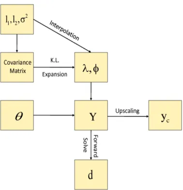
Fig. 2. Flow-chart for the hierarchical model.
Theorem II.2.1. Suppose Al be the covariance matrix for a given correlation length,
l. Let λ1, λ2. . . , λm be the m ordered eigen values considered in the K-L expansion
of Al and let φ1, φ2. . . , φm be the corresponding orthonormal eigen vectors. Suppose
Al+δl be the covariance matrix if we perturb the correlation lengthl by a small quantity
δl. Let λ′1, λ ′ 2. . . , λ
′
m be the m ordered eigen values considered in the K-L expansion
and let φ′ 1, φ
′ 2. . . , φ
′
m be the corresponding orthonormal eigen vectors. then,
λ′i =λi+O(δl), and φ ′
i =φi+O(δl), ∀i. (2.26)
The proof is given in Appendix B using matrix perturbation Theory.
The hierarchical model and the MCMC procedure is described by a simple graphical model on Figure 2.
II.3. Extension to Model with Unknownm
In the previous analysis, m, the dimension of θ remained fixed, so the number of the terms retained in K-L expansion is taken to be a constant. Usually it has been estimated by using equation (2.6). This method only utilizes the fine scale direct data yo but ignores the output data d and the coarse scale data yc. That way this
approach may not capture the actual heterogeneity of the spatial field very well. We extend our previous model by treatingm as an additional model unknown and obtain its posterior distribution by conditioning on all the available data. In this situation, we develop the Bayesian hierarchical model by extending equation (2.17) as
P(m, θ, l1, l2, σ2|d, yc, yo) ∝ P(d|m, θ, l1, l2, σ2)P(yc|m, θ, l1, l2, σ2)
× P(yo|m, θ, l1, l2, σ2)P(θ|m)p(m)P(l1, l2)P(σ2).(2.27)
We keep all the model specifications same as in Subsection II.1 but use a truncated Poisson prior for P(m). We need to modify the MCMC computation procedure due to this unknown dimension. If we vary the number of terms in K-L expansion then the dimension of θ will also change in each step. This jumping between different dimensions in the parameter space can be achieved through reversible jump Markov Chain Monte Carlo methods as proposed by Green (1995). We describe the reversible jump MCMC procedure in our case following the general approach of the reversible jump MCMC (Waagepetersen and Sorensen (2001)).
In our case using the hierarchical Bayes’ model, the posterior can be written as π(τ, m) ∝ P(d|θ, l1, l2, σ2, m)P(yc|θ, l1, l2, σ2, m)
× P(yo|θ, l1, l2, σ2, m)P(l1, l2)P(σ2)P(θ|m)P(m). (2.28)
λ ∼ Gamma(ν, β). Integrating out λ we get P(m) ∝ (1/β+1)1(m+ν+1). All the other terms remains same as in (2.18).
Algorithm: Reversible Jump MCMC as Birth and Death Process.
Suppose at therth step we are at the state (m
r, τr), then we have three possible steps:
• Birth Step. Propose to add the (mr + 1)th term in the K-L expansion with
probability pb
mr. Propose θ ′
from q(.) and hence θ∗ = (θ
r, θ ′
). The acceptance probability is given by αmr,mr+1(θr, θ∗) = min{1,
π(θ∗
,mr+1)pdmr+1
π(θr,mr)pbmrq(θ ′
)}.
• Death Step. Propose to delete the (mr)th term with probability pdmr. So here
(θ∗, θmr
r ) =θr. The acceptance probability is given by
αmr,mr−1(θr, θ∗) = min{1,
π(θ∗
,mr−1)pbmr−1q(θmrr )
π(θr,mr)pdmr }.
• Jump Step. Propose a new θ with the same dimension along withl1, l2, σ2 with
probability ps
mr. In other words generate τ
∗ from q(τ∗|τ
r). The acceptance
probability is given by α(τr, τ∗) = min{1,π(τ ∗ )q(τr|θ∗) π(τr)q(τ∗|τr))}. Where,pb mr+p d mr +p s mr = 1,∀mr.
II.4. Two Stage Reversible Jump MCMC
The main disadvantage of the above reversible jump MCMC algorithm is the high computational cost in solving the forward model on the fine-grid to computeGin the target distribution π(τ, m). Typically, in our simulations, reversible jump MCMC method converges to the steady state after several iterations. That way, a large amount of CPU time is spent on simulating the rejected samples, making the direct (full) reversible jump MCMC simulations very expensive.
The direct reversible jump MCMC method can be improved by adapting the proposal distribution q(τ, m|τn, mn) to the target distribution using a coarse-scale
model. This can be achieved by a two-stage reversible jump MCMC method, where we compare the output from the forward model on a coarse-grid , first. If the pro-posal is accepted by the coarse-scale test, then a full fine-scale computation will be conducted and the proposal will be further tested as in the direct reversible jump MCMC method. Otherwise, the proposal will be rejected by the coarse-scale test and a new proposal will be generated from q(τ, m|τn, mn). The coarse-scale test filters
the unacceptable proposals and avoids the expensive fine-scale tests for those propos-als. The filtering process essentially modifies the proposal distribution q(τ, m|τn, mn)
by incorporating the coarse-scale information of the problem. The algorithm for a general two-stage MCMC method with upscaling was introduced in Efendiev et al. (2007). Our hierarchical model can also take an advantage of inexpensive upscaled simulations to screen the proposals. Here we extend the algorithm to two-stage re-versible jump MCMC method. LetF∗
τ be the output computed by solving the forward
model on a coarse-scale for the given fine-scale spatial field with parameters (τ, m). In the case of Reservoir characterization this is done either with upscaling methods or mixed MsFEM. The fine-scale target distribution π(τ, m) is approximated on the coarse scale by π∗(τ, m). Here all the terms in the expression of π∗(τ, m) is same as that of π(τ, m) except only the likelihood term 1
[bf+12||d−Fτ||2] (af+n/2) is replaced by 1 [bf+12H||d−F ∗ τ||2]
(af+n/2). Where the function H is estimated based on offline computa-tions using independent samples from the prior. More precisely using independent samples from the prior distribution, the spatial fields are generated. Then both the coarse-scale and fine-scale simulations are performed and kd−Fτk vs kd−Fτ∗k are
plotted. This scatter plot data can be modeled by kd−Fτk = H(kd−Fτ∗k) + w,
where w is a random component representing the deviations of the true fine-scale error from the predicted error. Using the coarse-scale distribution π∗(τ) as a filter, the two-stage reversible jump MCMC can be described as follows.
Algorithm: Two-stage reversible jump MCMC as Birth and Death Pro-cess.
Suppose at thenth step we are at the stateν
n. Letkn be the corresponding fine-scale
permeability field. Here νn = (τn, mn).
• Step 1. This step is the same as the reversible jump MCMC method described earlier. The only difference is the fractional flow F∗
ν is computed by solving the
coarse-scale model. At νn, generate a trial proposal ˜ν from distribution q(˜ν|νn)
the same way as in the reversible jump MCMC described earlier i.e this step is same as doing reversible jump MCMC on π∗(ν).
• Step 2. Take the proposal as
ν= ˜ ν with probability αp(νn,ν),˜ νn with probability 1−αp(νn,ν).˜
If we are at Birth Step then the acceptance probability is given by αp(νn,ν) =˜ min{1, π∗(˜τ , m n+ 1)pdmn+1 π∗(τn, mn)pb mnq(θ ′ )}. (2.29)
If we are at death step then the acceptance probability is given by αp(νn,ν) =˜ min{1, π∗(˜τ , m n−1)pbmn−1q(θ mn n ) π∗(τn, mn)pd mn }. (2.30)
If we are going to have only jumps then the acceptance probability is given by αp(νn,ν) =˜ min{1,
π∗(˜τ , m
n)q(τn|τ˜)
π∗(τn, mn)q(˜τ|τn))}. (2.31) • Step 3. Accept ν as a sample with probability
αf(νn, ν) = min 1, Q(νn|ν)π(ν) Q(ν|νn)π(νn) . (2.32)
Where, Q(ν|νn) is the transition kernel of the first stage. The acceptance
prob-ability (2.32) can be simplified as αf(νn, ν) = min 1,π(ν)π∗(νn) π(νn)π∗(ν) . (2.33)
To show that the two stage reversible jump MCMC sampling generates a Markov chain, whose stationary distribution is the candidate distribution it is sufficient to show that the transition kernel satisfies the detailed balance condition.
Theorem II.4.1. If K(νn, ν) is transition kernel of the Markov Chain νn generated
by the two-stage reversible jump MCMC, then
π(νn)K(νn, ν) =π(ν)K(ν, νn). (2.34)
The proof is given in the Appendix C.
II.5. Simulated and Real Examples from Reservoir Model
For definiteness our examples are focused on petroleum reservoir models. However the developed theory, methodology and the computation tools will be useful for any inverse problem in spatial and temporal field with large scale simulator. Reservoir simulation models are widely used by oil and gas companies for production forecasts and for making investment decisions. If it were possible for Geo scientists and engi-neers to know the physical properties like locations of oil and gas, the permeability, the porosity, and the multi-phase flow properties at all locations in a reservoir, it would be conceptually possible to develop a mathematical model that could be used to predict the outcome of any action. This model is usually a set of partial dif-ferential equations. If the model variables are known, outcomes (output variables) can be predicted, usually running a numerical reservoir simulator that solves a
dis-cretized approximation to those partial differential equations. This is the forward problem. Unfortunately, most oil and gas reservoirs are inconveniently buried be-neath thousands of feet of overburden. Direct observations of physical properties of the reservoir are available only at a few well locations. Additionally, we have some indirect observations known as the production data (the output data d) which are typically made at the surface, either at the well-head or at distributed locations. The main intention is to determine the plausible physical properties of the reservoir given these direct and indirect observations. This is an inverse problem and the solution of the inverse problem provides an estimate of the characteristics of the subsurface media. In order to solve this inverse problem, the mismatch between simulated (from the numerical reservoir simulator) and observed measurements of production data is minimized. This method is known as the history matching in petroleum engineering. The characteristics of the subsurface media are quantified by several parameters such as permeability, porosity, fluid saturation etc., which are the major contributors to the uncertainties in reservoir performance forecasting. Large uncertainties in reser-voirs can greatly affect the production and decision making on well drilling. Better decisions can be made by reducing the uncertainty. Thus, quantifying and reducing the uncertainty are important and challenging problems in subsurface modeling. In the following examples, we are particularly interested in quantifying and reducing the uncertainties for one of the major characteristics of subsurface property, permeability. Hence we need to infer about the permeability spatial filed based on the direct and indirect observations. The fine-scale data represent point measurements such as well logs and cores where as the coarse-scale data are obtained from seismic traces. First, we perform simulation studies to explore the behavior of our modeling approach.
II.5.1. The Mathematical Model and Specification ofG
The model has been described in Subsection I.1.1 as d = logit[G(Y)] +ǫ. Where d is the watercut data, Y is the fine-scale permeability field expressed in a logarithm scale, i.eY =log(kf) andGis simulator output by using the log-permeability fieldY.
G is determined by the Darcy’s law and given by the following PDEs. We consider two-phase flow in a subsurface formation over a bounded set D ⊂ R2 under the
assumption that the fluid displacement is dominated by viscous effects. For clarity of exposition, we neglect the effects of gravity, compressibility, and capillary pressure, although our proposed approach is independent of the choice of physical mechanisms. Also, porosity φ will be considered to be known constant. The two phases will be referred as the water and the oil (or a non-aqueous phase liquid), designated by subscripts wand o, respectively. Darcy’s law for each phasej, (j =w, o) is given by
vj =−
krj(S)
µj
kf∇p, (2.35)
where, vj =vj(x, t), (x, t) ∈D×[0,∞) , is the phase velocity at time t and spatial
location x. µj is the dynamic viscosity and kf = kf(x), x ∈ D, is the fine-scale
permeability field. S = S(x, t), (x, t) ∈D×[0,∞), is the water saturation (volume fraction) and krj = krj(S(x, t)), (x, t) ∈ D×[0,∞) is the relative permeability to
phase j (j = o, w). For simplicity, here we take krw = S2 and kro = (1 − S)2.
p = p(x, t), (x, t) ∈ D× [0,∞), is the pressure and ∇is the differential operator
∂(.) ∂x1, ∂(.) ∂x2
. Combining the Darcy’s law with a statement of conservation of mass allows us to express the governing equations in terms of pressure and saturation equations:
∇ ·(λ(S)kf∇p) = q1, (2.36)
φ∂S
∂t +v· ∇f(S) = −q2, (2.38)
where, λis the total mobility λ(S) = krw(S)
µw +
kro(S)
µo ,f is the fractional flux of water ,
f(S) = krw(S)/µw
krw(S)/µw+kro(S)/µo,v is the total velocity,q1 andq2 are known source term (for
simplicity we assumeq1 = 0). The above descriptions are referred to as the fine-scale
model of the two-phase flow problem. The p.d.e’s (2.36)-(2.38), are solved with the following boundary conditions. The pressurepis taken to be known at the boundaries ofD, i.ep=q3 for (x, t)∈∂D×[0,∞), where q3 is known. The initial conditions for
S are specified for t= 0. We partition ∂D into three parts ∂Din, ∂Dout and ∂Dother,
i.e,∂D=∂Din∪∂Dout∪∂Dother. Where, water in injected on∂Din and the fluid (oil
and water) are produced on ∂Dout, also called the production edge. So the boundary
condition on S is taken as S = 1 on ∂Din. Solving the p.d.e’s (2.36)-(2.38) with
the above boundary condition for a known permeability field kf(x) would yield the
solution of v(x, t) and S(x, t) ∀(x, t). The fractional flow or the water-cut at time t is defined as the the fraction of water in the produced fluid on the production edge ∂Dout and is given by:
F(t) = R ∂Doutvnf(S(x, t))dx R ∂Doutvndx , (2.39)
where, vn is the component of the velocity field v which is normal to the boundary
∂Doutanddxdenotes that the integration is taken along the boundary. The fractional
flow or water-cut at time t, F(t) depends on the total velocity v and the water saturation S, which are the solutions of the pde’s (2.36)-(2.38) for a given spatial permeability fieldkf(x) = exp(Y(x)) with some boundary conditions on S and p. In
other words Y(x) is the input and F(t) is the output for the forward simulator. So F(t) can be written as F(t) = G(Y(x)). Since F(t) is always between 0 and 1 we
take a logit transformation onG and write the forward model as:
d=logit(G(Y(x))) +ǫ. (2.40)
II.5.2. The Upscaling Procedure
Fig. 3. Schematic description of fine- and coarse-grids. Bold lines illustrate a coarse-s-cale partitioning, while thin lines show a fine-scoarse-s-cale partitioning within coarse– grid cells.
Consider the fine-scale spatial field which is defined in the domain with under-lying fine grid as shown in Figure 3. On the same graph we illustrate a coarse-scale partition of the domain. Here we consider single-phase flow upscaling procedure for two-phase flow in heterogeneous porous media (see Efendiev et al.(2005)). To calcu-late the upscaled spatial field at the coarse-level, we use the solutions of local pressure equations. The main idea of the calculation of a coarse-scale permeability is that it delivers the same average response of the forward model as that of the underlying fine-scale problem locally in each coarse-block. For each coarse domain K, we solve
the local pressure equations in the fine grid
v =−kf(x)∇p, ∇.(v) = 0, (2.41)
with some coarse-scale boundary conditions. Here kf(x) denotes the fine-scale
per-meability field, p is the pressure, v is the velocity and ∇ is the partial differential operator ∂(.)∂x
1,
∂(.) ∂x2
. The pressure equations in (2.41) can be also written together as:
div(kf(x)∇p) = 0. (2.42)
The approach considered here is to replace kf with upscaled coarse permeabilities,
kc, which is constant in each fine grid within the same coarse block. By definition
kc is a discrete quantity relying on the discretization of the medium. In particular,
kc depends on the location and geometry of the grid-block in which it is computed.
The essential requirement of kc is that it leads to pressure and velocity solutions with
desired accuracy so that the average response of the forward model in each coarse domain is almost same as the response from the fine-scale model. kc is defined in a
given coarse blockK such that
kch∇p∗iK =− hv∗iK, (2.43)
where p∗ and v∗ are the solutions of (2.41) (with appropriate boundary conditions, discussed below), and h.iK = |K1|RK(.)dx is the block average over K. In two di-mensional setting we solve two independent local fine scale solutions v∗
i and p∗i of the
pressure equations
vi =−kf(x)∇pi, ∇.(vi) = 0. (2.44)
in each coarse blocksK, i= 1,2, with a given boundary condition. Letei be the
pi = 0 on the opposite sides along the direction ei and no flow boundary conditions
on all other sides, i.e vi.n= 0, along the direction ej, (j 6=i) (as shown in Figure 3),
where, vi.n is the component of the velocity field vi which is normal to the boundary
∂D. For these boundary conditions, the coarse-scale permeability tensor is given by ei.kcej = 1 |K| Z K (∇p∗i(x).kf(x)∇p∗j(x))dx, (2.45) where p∗
i and p∗j are the solution of (2.41) with corresponding boundary conditions.
Various boundary condition can have some influence on the accuracy of the calcu-lations, including periodic, Dirichlet etc. (see Wu et al. (2002)). In our numerical examples we take the logarithm of the observed coarse scale permeability as our coarse data, i.e yc =log(kc).
II.5.3. Numerical Results for Simulated Reservoirs
In our first example, we have considered only the isotropic case, i.e we takel1 =l2 =l,
(say). We consider a 50×50 fine-scale permeability field on the unit square. We gener-ate 15 fine-scale permeability field withl =.25,σ2 = 1 and the reference permeability
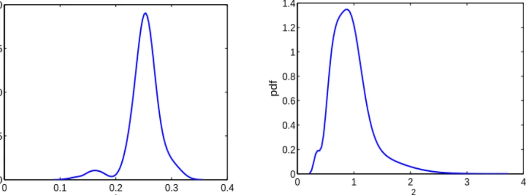
field is taken to be the average of these 15 permeability field. The fractional flow or water cut data is generated from the reference permeability field using eclipse software and was validated by the petroleum engineering department. The observed coarse-scale permeability field is calculated using the upscaling procedure in a 5×5 coarse grid. The fine-scale permeability field is observed at 6 locations along x = 0 and x = 1 boundaries. First we implement the reversible jump MCMC algorithm. We take the first 20 terms in the K-L expansion while generating the reference field. The mode of the posterior distribution of m comes out to be 19. The posterior mean of fine-scale permeability field resembles very close to the reference permeability field. The mode of the posterior density of l is near 0.25. The posterior density σ2 are
centered around 1. So, the posterior density ofσ2 and l have peak corresponding to
the values of the generated reference field. Then we implement two-stage reversible jump MCMC algorithm with the same reference field and water cut data as we have used in the reversible jump MCMC. The two-stage reversible jump MCMC produced the same results as in reversible jump MCMC (see Figures 4, 5 and 6). The two-stage algorithm is much faster as it rejects the bad samples in the first-stage where we solve the partial differential equations on a coarse grid. The effective acceptance rate of the two-stage algorithm increases to almost eighty percent where as the regular Re-versible Jump MCMC have a acceptance rate of nearly ten percent. Then we consider a case where we assume that no coarse-scale data is available but ten percent of the fine scale data are available at equidistant point. We proceed with the same reference permeability field and same water-cut data. The results are plotted on Figure 7. The same procedure is replicated assuming twenty five percent data available (see Figure 8). We can see that if coarse-scale data is not available ten percent fine scale data is not enough to capture the parameters of the model, we need at least twenty-five percent of the fine-scale data.
II.5.4. Numerical Results for a Real Field Example
In this subsection we apply our model on a real field example , viz. punq-s3 model dataset. The PUNQ-S3 case has been taken from a reservoir engineering study on a real field performed Elf Exploration Production. It was qualified as a small-size industrial reservoir engineering model. The model contains 19×28×5 grid blocks. The PUNQ-S3 data set was an experimental study where the true permeability was actually known on the 19×28×5 grid but the researchers were asked not to use the permeability data for their modeling purpose. They were asked to use the production history only to infer about the true permeability field and then compare how their
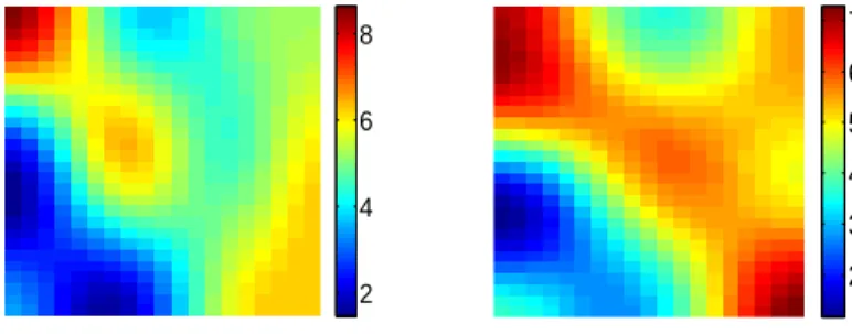
reference fine−scale log−permeability field initial fine−scale log−permeability field
observed coarse−scale log−permeability field
0.6 0.8 1 1.2 1.4 1.6 posterior median −0.5 0 0.5 −0.5 0 0.5 −1 −0.5 0 0.5 1
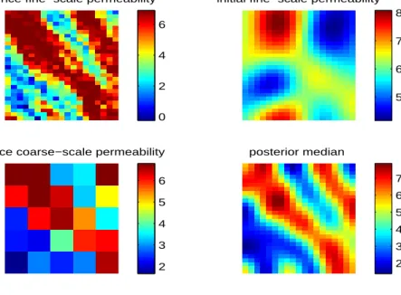
Fig. 4. Log permeability plot for the simulated example using two stage reversible jump MCMC. Top left: The true fine-scale log permeability field. Top right: Initial fine-scale log permeability field. Bottom left: The observed coarse-s-cale permeability field. Bottom Right: The median of the sampled fine-scoarse-s-cale permeability field. 15 20 25 30 0 50 100 150 200 250 300 350 400 450 frequency m
Histogram of the posterior mass function of m
Fig. 5. Histogram of the posterior distribution of m for two-stage reversible jump MCMC.