Learning from Simulation to Improve Robotic Sensing

(1)

M a s te ra rb e it

Amrutha Saseendran

Learning from Simulation

to improve Robotic Sensing

Learning from Simulation to

Improve Robotic Sensing

(2)

Institut für Robotik und Mechatrorfüc

BJ.: 2019

IB.Nr.: DLR-IB-RM-OP-2019-56

MASTERARBEIT

LEARNING

FROM SIMULATION

TO

IMPROVE

ROBOTIC

SENSING

Freigabe: DerBearbeiter: Unterschriften

AmruthaSaseendran

CA"

-"a

/ ,!: / Betreuer: I i

,

( .l Zoltän-Csaba Märton ,'

l"/"l,

]./

a

l

:reorf"".Alsi:nfüAl'ab"u-"'Scohräffer

(A!"{J2L

Dieser Bericht enthält 95 Seiten, 50 Abbildungen und 3 Tabellen

(3)

Institut für Theoretische Elektrotechnik und

Mikroelektronik

Universität Bremen

Master Thesis

Learning from Simulation to Improve

Robotic Sensing

Amrutha Saseendran

Control Microsystems and Microelectronics

Universität Bremen

Matriculation Number: 3062300

Supervisors:

Dr. Zoltán-Csaba Márton

Dipl.-Inf. Manuel Brucker

M.Sc Martin Sundermeyer

Institute for Robotics and Mechatronics, German Aerospace Centre (DLR)

Prof. Dr.-Ing. Alberto Garcia-Ortiz

Chair for Integrated Digital Systems, ITEM

Prof. Michael Beetz PhD

Head of the Institute for Artificial Intelligence, University of Bremen

March 2019

(4)

(5)

Acknowledgement

This thesis work was carried out in the year 2018/19 at the German Aerospace Center (DLR), at the Institute of Robotics and Mechatronics.

Foremost, I would like to thank my advisors at the DLR, Dr. Zoltán-Csaba Márton, Manuel Brucker and Martin Sundermeyer for their supervision, motivation, support and granted freedom. Their guidance helped me throughout my research and writing of this thesis. Furthermore, I would like to express my sincere gratitude to my university supervisors Prof. Dr.-Ing. Alberto Garcia-Ortiz and Prof. Michael Beetz PhD, for the supervision, advice and smooth execution of my thesis.

I am grateful to Prof. Dr.-Ing. Alin Albu-Schäffer, Head of the Institute of Robotics and Mechatronics at the DLR, for the opportunity to carry out this work in the department of Perception and Cognition.

I would also like to express my personal thanks for a lot of useful discussions to Ferenc Bálint-Benczédi.

(6)

(7)

Abstract

The ability of the robot to sense its environment is essential for its autonomous operation. Precise object detection and pose estimation, derived from the sensing capabilities, is crucial for the autonomy of any robotic system. Deep learning and neural networks have already revolutionized this field. The research community has successfully developed powerful deep learning algorithms using neural networks for faster and accurate object detection and pose estimation. However, these methods require a large amount of annotated dataset for the training of neural networks. Preparation of such high quality annotated dataset is expensive and time-consuming. An alternative method is to make use of the easily available simulation data instead of real data for training. Because of the domain gap between the simulation and the real data, networks trained with simulation data fails to perform well on real images.

This thesis explores the possibility of generating realistic looking images using Generative adversarial network (GAN), in order to overcome the existing domain gap between the simulated and real images. Recent research on GANs has shown that these networks are capable of producing photo-realistic images and is a promising new area of the research field for producing realistic synthetic images. Inspired from one of the variants of GAN known as CycleGAN, the proposed work explores the possibility of generating realistic images from simulated images using modified CycleGAN architecture. Using the T-LESS and YCB dataset as the benchmark, the generated images are then evaluated by training an object detector network. The quality of the generated images are measured by the accuracy of the detector and then compared with the real domain images.

(8)

(9)

List of Figures

1.1 Generative Model . . . 14

1.2 All T-LESS Objects . . . 17

1.3 All YCB Objects . . . 17

2.1 SSD Architecture . . . 22 2.2 Retinanet Architecture . . . 22 3.1 Structure of Generator . . . 25 3.2 Structure of Discriminator . . . 26 3.3 GAN Architecture . . . 26 3.4 CoGAN Architecture . . . 29 3.5 CycleGAN Illustration . . . 30 4.1 Generator Architecture . . . 34

4.2 Generator layer specifications . . . 34

4.3 Resnet Block Illustration . . . 35

4.4 Discriminator Architecture . . . 35

4.5 Discriminator layer specifications . . . 36

4.6 CycleGAN Architecture . . . 37

4.7 CycleGAN Architecture with mask loss . . . 38

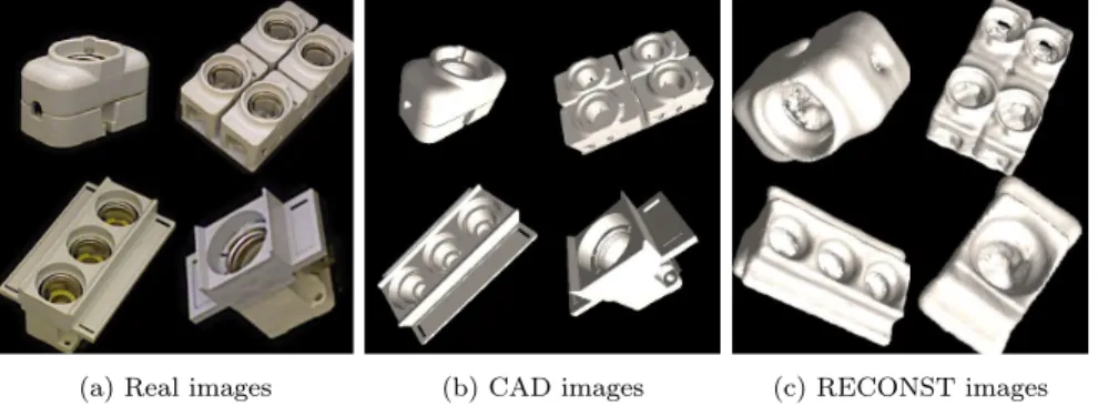
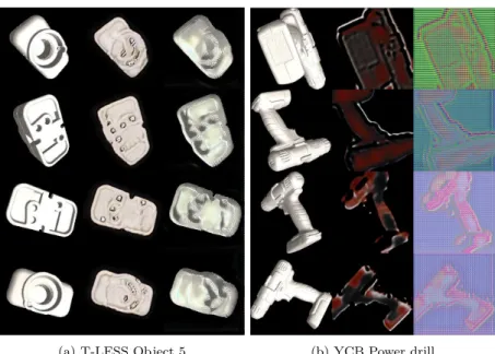
5.1 T-LESS dataset objects in different domains. Clockwise from top, Object 5, Object 8, Object 9 and Object 10 . . . 44

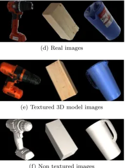
5.2 YCB objects used for evaluation. From left, power drill,wood block and pitcher base 45 (d) Real images . . . 45

(e) Textured 3D model images . . . 45

(f) Non textured images . . . 45

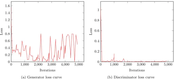
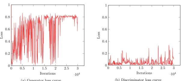
5.3 Loss curve during Vanilla CycleGAN training. The values represent the corresponding loss function values for each iterations. . . 47

5.4 Results obtained from Vanilla CycleGAN architecture. The rendered CAD models of the object used as input is shown in left column, the corresponding output from the generator is shown in the middle column and the reconstructed image is shown in the right column. . . 48

5.5 Loss curve of CycleGAN with patch discriminator. The values represent the corresponding loss function values for each iterations. . . 49

(13)

List of Figures

5.6 Results obtained when patch discriminator architecture is used. The rendered CAD models of the object used as input is shown in left column, the corresponding output from the generator is shown in the middle column and the reconstructed image is

shown in the right column. . . 50

5.7 Loss curves of CycleGAN when generator network is trained more number of times than discriminator. The values represent the corresponding loss function values for each iterations. . . 51

5.8 Results obtained when generator network is trained more number of times than discriminator. The rendered CAD models of the object used as input is shown in left column, the corresponding output from the generator is shown in the middle column and the reconstructed image is shown in the right column. . . 52

5.9 Loss curves of CycleGAN when identity loss function is added to the generator loss function. The values represent the corresponding loss function values for each iterations. . . 53

5.10 Results obtained when identity loss function is added to the generator loss function of the network. The rendered CAD models of the object used as input is shown in left column, the corresponding output from the generator is shown in the middle column and the reconstructed image is shown in the right column. . . 54

5.11 Effect of dropout layers in a standard neural network . . . 55

5.12 Loss curves of CycleGAN when dropout layers are added to discriminator network. The values represent the corresponding loss function values for each iterations. . . . 56

5.13 Results obtained when dropout layers are added to the discriminator architecture of the network. The rendered CAD models of the object used as input is shown in left column, the corresponding output from the generator is shown in the middle column and the reconstructed image is shown in the right column. . . 57

5.14 An example image of T-LESS object 5 with generated image position deviated from the input image . . . 57

5.15 Loss curves of CycleGAN when mask loss function is added to the generator loss function.The values represent the corresponding loss function values for each iterations. 58 5.16 Results obtained when mask loss function is added to the generator loss function of the network. The rendered CAD models of the object used as input is shown in left column, the corresponding output from the generator is shown in the middle column and the reconstructed image is shown in the right column . . . 58

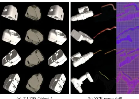
5.17 Results obtained for T-LESS object 8 using our CycleGAN architecture. . . 59

5.20 Results obtained for YCB object wood block using our CycleGAN architecture. . . . 60

5.21 Results obtained for YCB object pitcher base using our CycleGAN architecture. . . 61

5.22 Sample T-LESS input images in various domains used for training the RetinaNet object detector. . . 62

5.23 Object detection results on different combinations of real and GAN images from table 5.1 and 5.2. The number of real images used for training the detector is expressed in percentage. The mAP values obtained for each percentage of input real images are plotted. . . 63

5.24 Comparison of real and GAN generated images of T-LESS objects. . . 63

(14)

List of Figures

5.25 Sample YCB input images from various domains used for training the RetinaNet object detector. . . 64 5.26 Comparison of real and GAN generated images of YCB objects. . . 65 A.1 Object detection results of T-LESS object 5 shown in red bounding box; tested on

T-LESS test scene 11 . . . 81 A.2 Object detection results of T-LESS object 8 shown in orange bounding box; tested

on T-LESS test scene 11 . . . 82 A.3 Object detection results of T-LESS object 9 shown in blue bounding box; tested on

T-LESS test scene 11 . . . 83 A.4 Object detection results of T-LESS object 10 shown in dark blue bounding box;

tested on T-LESS test scene 11 . . . 84 A.5 Object detection results of YCB object power drill shown in red bounding box;

tested on YCB video dataset extracted images . . . 85 A.6 Object detection results of YCB object wooden block shown in orange bounding

box; tested on YCB video dataset extracted images . . . 86 A.7 Object detection results of YCB object pitcher base shown in blue bounding box;

(15)

List of Tables

5.1 Object detection results on objects 5,8,9 and 10 of T-LESS dataset. The mAP values obtained for various domains of input images using RetinaNet detector is

tabulated. Higher values of mAP corresponds to better performance. . . 61 5.2 Object detection results on objects 5,8,9 and 10 of T-LESS dataset. The mAP

values obtained for various combinations of real and GAN images using RetinaNet detector is tabulated. Higher values of mAP corresponds to better performance. . . 62 5.3 Object detection results on objects power drill, wood block and pitcher base of

YCB dataset. The mAP values obtained for various combinations of input images using RetinaNet detector is tabulated. Higher values of mAP corresponds to better performance. . . 64

(16)

List of Abbreviations

AI Artificial Intelligence

AIMM Autonomous Industrial Mobile Manipulator

BN Batch Normalization

CAD Computer Aided Design

C-GAN Conditional GAN

CNN Convolutional Neural Network

CoGAN Coupled GAN

CPU Central Processing Unit

CUDA Compute Unified Device Architecture

DC-GAN Deep Convolutional GAN

DLR Deutsches Zentrum für Luft-und Raumfahrt

FPN Feature Pyramid Network

GAN Generative Adversarial Network

GPU Graphical Processing Unit

HOG Histogram of Oriented Gradients

IN Instance Normalization

MAE Mean Absolute Error

mAP Mean Average Precision

MSE Mean Squared Error

PixelRNN Pixel Recurrent Neural Network

R-CNN Region based CNN

R-FCN Region based Fully Connected Network

RoI Region of Interest

RPN Region Proposal Network

SSD Single Shot Detector

SVM Support Vector Machine

T-LESS Texture-less

VAE Variational Autoencoder

YCB Yale-CMU-Berkeley

(17)

(18)

Chapter 1 Introduction

In order to enable robots to interact with their environment, the semantic gap between raw sensory data and meaningful representation of their surroundings needs to be overcome. For example, the humanoid robot DLR Justin [1] needs to interact with household objects and DLR AIMM [2] (Autonomous Industrial Mobile Manipulator) executes fetch and carry operations in unstructured environments. For robotic manipulation, fast and accurate object detection and pose estimation is essential.

Object detection is one of the classical research areas in computer vision and Artificial intelligence (AI), which has improved rapidly in the recent years. It deals with the problem of detecting and localizing objects in an image and predicting the bounding box of the objects of interest in the scene. Many approaches have been proposed for object detection, from traditional computer vision techniques to modern deep learning architectures. Learning-based methods like Convolutional neural networks (CNNs) have revolutionized this field of research [3]. Modern network architectures along with advanced computing technology have successfully enabled object detectors that surpass human performance. These models can accurately predict bounding boxes and class labels of objects in various environments. However, they require large amounts of labeled data during training to achieve the desired performance.

Why is the training data an important factor in deep learning? Deep learning models have a huge amount of parameters to tune and require a large dataset to produce a generalizable model. The efficiency of training a deep learning model depends on the quality of the training data provided. In real-world applications, there is little chance, that the objects of interest are part of a publicly available dataset. Therefore, the dataset for training the network has to be acquired manually which is often not practical and can be expensive. An alternative and promising method to overcome this problem is to use artificial or synthetic data. Generating synthetic data that replicates real-world data would help to transfer the impressive results achieved with deep learning to real-world applications. Synthetic data can be used for many applications like image inpainting [4], reinforcement learning [5], digital image enhancements, and natural language processing [6].

(19)

Chapter 1. Introduction

networks trained with synthetic data fail to match the detection performance of their counterparts trained with natural images. This so-called domain gap between synthetic and real dataset is a major challenge faced when using synthetically trained networks. A Generative model is an effective method of learning any kind of data distribution. These models have recently shown advances towards the goal of generating realistic synthetic data and are further explained in the next section of the chapter.

1.0.1 Generative Models

In general, machine learning models are categorized either as generative or discriminative models. Discriminative models try to classify or distinguish the data distribution whereas generative models try to model the underlying data distribution. In other words, ifyis an output variable for a given input sample x then, discriminative models try to model the conditional/posterior probability p(y|x), whereas generative models try to learn the joint probability function p(x,y). Depending upon the application one of these models is chosen appropriately.

Generative models focus on how the given data is generated. For example consider a dataset of samples x1, x2, x3, ..., xn sampled from a true data distribution p(x) as shown in Fig 1.1. The

blue region in the figure corresponds to the region in image space that contains real images in the training dataset and the black dots indicates the images in the dataset. The generative model implicitly defines another data distribution p(ˆx) by mapping the points from the unit Gaussian distribution z through the neural network. The neural network is basically a function with parameterθ and this parameter is used to control the generated data distributionp(ˆx). The distribution p(ˆx) starts randomly and then during the training process by updating θ, the model tries to minimize the differences between the true and the generated distribution. In short, the objective here is to find the parameterθthat produces no difference between the two distributions. Generative models do not produce the output by merely reproducing the data distribution but discovers the inherent characteristics in a data distribution and learns the underlying structure.

Figure 1.1: Generative model (adapted from [7]).

(20)

These models are thus one of the most promising approaches to understand and perceive the visual world around us. Three popular deep generative models are General Adversarial Networks (GANs) [8], Variational Autoencoders [9] (VAEs) and Pixel Recurrent Neural Networks (PixelRNNs) [10]. Generative adversarial networks comprise of two neural networks known as generator and discriminator. The generator generates images from input random noise and the discriminator tries to distinguish the real dataset from the generator’s output to classify real and fake data. These two networks are trained simultaneously, where the generator tries to generate images close to the real images making it difficult for the discriminator to distinguish. This is often termed as a two-player mini-max game between generator and discriminator. VAEs use a probabilistic graph model based on Bayesian inference in which the probability distribution of the data is modeled to produce a new sample from the distribution. PixelRNNs are autoregressive neural networks that generate models which predict the conditional distribution of the pixels in an image when previous pixels are given. In this method, the model scans the image, one row and one pixel (within each row) at a time and predicts the distribution over the possible values for the next pixel. PixelRNNs are often used in image completion applications.

Recent research on GANs shows their ability to generate photorealistic images. It is also known to produce sharper images compared to the other generative models like VAE and PixelRNNs. The working principle of GANs is to reduce the distinguishability between the generated and the real data distribution. Because of the game theory approach and the brittle structure of GANs, they are well-known to be tricky to train. A lot of research in GANs is focused on understanding the reasons for this difficulty and the methods to reliably reach convergence.

1.1 Problem Formulation and Research Objective

This thesis focuses on the task of using synthetic images generated from generative adversarial networks for training object detectors. The major problems that we investigate are formulated as follows:

• The existing domain gap between real and synthetic images. • The difficulty in stabilizing the training process of GANs. The following aspects are evaluated as a part of this research:

• The state of the art generative adversarial networks for synthetic image generation • The applicability of GANs to generate synthetic images that resemble real data.

• The possibility of training object detectors with generated synthetic images and no (or as few as possible) real data.

(21)

1.2 Methodology

The proposed research is an evaluation of GANs for synthetic image generation and explores their potential using the generated data to train object detectors. However, since the training of GANs can be challenging, suitable training methods are adopted and are further explained in chapter 4. The proposed method will use rendered 3D Computer Aided Design (CAD) models of the objects to be detected and real images as input to the generative model for augmenting the rendered images. The generated synthetic images are then used for training object detectors. The thesis is structured as follows:

• Investigate the potential of GAN for domain adaptation.

•Generate realistic images from CAD rendered images preserving the label information using GAN. • Evaluate the generated images quality by training an object detector.

•Compare the performance of the object detector using real images, GAN generated images, CAD rendered images and combination of real and GAN images.

1.3 Framework

1.3.1 Tensorflow

Tensorflow is an open source machine learning library developed by the Google brain team and is extensively used nowadays for research and industrial purposes [11]. It was initially used by Google for internal research and production purposes. It was later released under Apache 2.0 license in November 2015. In Tensorflow, computations are done in data flow graphs where a node represents mathematical operations and edges represent multidimensional arrays called tensors. Tensorflow supports Central Processing Unit (CPU), Graphical Processing Unit (GPU) and distributed processing. The architecture of Tensorflow is highly flexible, modular and portable. It also aids easy visualization of complex neural networks. In this thesis Tensorflow version, 1.8 is used.

1.4 Datasets

In order to evaluate the network model, we use T-LESS [12] and YCB datasets [13].

1.4.1 T-LESS

T-LESS is a dataset consisting of a collection of 30 industry-relevant texture-less objects captured from a systematically sampled view sphere with 10-degree steps in elevation and 5-degree steps in azimuth [12]. This RGB-D dataset is used for the SIXD challenge for object detection and pose estimation. The dataset comprises of objects recorded using three different sensors: a Microsoft Kinect v2, a Canon IXUS 950 IS camera and a Primesense Carmine RGB-D sensor. Moreover, it contains manually created and semi-automatically reconstructed CAD models of the objects. The Dataset also includes per-image bounding-box values of the objects with annotations of the form

(22)

Figure 1.2: All T-less objects.

(x,y,x+w,y+h) where w and h are the width and height of the bounding box and the coordinate (x,y) is the upper left corner of the bounding box. Figure 1.2 shows the 30 T-LESS objects in ascending order. The T-LESS version v2 is used in this thesis.

1.4.2 YCB

Yale-CMU-Berkeley (YCB) dataset is a popular dataset used for robotic grasping and manipulation research. The dataset comprises of objects that are frequently used in daily life with varying sizes, shapes, textures, weight and rigidity. The database offers RGB-D images, high resolution RGB images, segmentation masks of the images, calibration information and 3D texture mapped mesh models [13]. The object set includes 77 objects that are widely used in manipulation tasks, divided in to 5 categories namely food, kitchen, shape, tool and task items. Figure 1.3 shows all 77 YCB objects. The dataset was prepared by using a scanning rig with 5 RGB-D sensors and 5 high resolution RGB cameras arranged in a quarter circular arc [13]. The objects were placed in a computer controllable turntable and then automatically rotated by 3 degrees at a time producing 120 turntable orientations.

(23)

(24)

Chapter 2 Related Work

This thesis focuses on generating synthetic images using GANs and to train object detectors with the generated images. Multiple approaches have been proposed for photorealistic image generation and this section covers information regarding some of the prominent works. This chapter includes the state of the art methods for synthetic image generation, Generative adversarial networks and then briefly reviews some of the well-known works in object detection to motivate our choice of object detectors.

2.1 Synthetic Images for Neural Networks

A great deal of work has been done to study the possibility of using synthetic datasets in image processing applications. Synthetic data usage has a well-established history in computer vision. An attempt by Nevatia et al. in which 3D CAD models were used for building object models is one of the earlier methods proposed in this field [14]. This work was proposed for solving the problem of scene analysis when multiple occluded objects are present or when specific objects in the scene are not known. The authors describe techniques to produce structured, symbolic description of complex curved objects in complex scenes by segmenting them into smaller subparts. The recognition is then further performed by comparing these descriptions with the stored description of 3D models of the objects. They demonstrated their results for a limited class of scenes. Several methods [15] [16] were proposed in which 3D CAD models were used as the labeled data for learning shape models to predict single object class like cars or motorcycles. Most of the proposed work uses a mixture of real and synthetic data to train neural networks. In [17] labeled image patches are used to generate synthetic images by using a method of cutting object instances and pasting them on a random background. Another approach by Hao Su et al. [18] uses 3D CAD models for viewpoint estimation using Convolutional neural networks. It out-performed the existing methods at that time on viewpoint estimation of 12 object classes from PASCAL 3D+[19]. A similar type of work was done by Peng et al. [20]. They used rendered 3D CAD models both textureless and with texture by varying projections and orientations of the objects in PASCAL VOC 2007 dataset [21]. Their work demonstrated that augmenting the training data for contemporary Deep Convolutional Neural Networks (DCNN) is effective when there are few training samples or when the dataset is not matched to the target domain. The authors also investigated the sensitivity of convnets to various low-level cues in the training dataset such as 3D pose, foreground and background texture,

(25)

Chapter 2. Related Work

and colour. The deep convnet trained for the detection task was highly invariant to these cues. The training of the convnet using the synthetic images with simulated cues achieved the same performance as training on synthetic images without the cues. However, the authors also suggest that further experiments with other domains are necessary since their findings were preliminary. One of the recent approaches by Georgakis et al. [22] evaluated the usage of synthetically generated composite images by superimposing 2D images of related objects in real environments at different positions and scale for object instance detection. They demonstrated their results in GMU-Kitchens and Washington RGB-D scenes v2 dataset. Using hand labeled dataset together with synthetically generated dataset they achieved comparable performance to using only manually labeled data. However, all these approaches rely on real data to achieve competitive performances. Stefan Hinterstoisser et al. [23] presented a method of training object detectors with synthetic data generated from rendered 3D models. They employed a technique of freezing the weights of a feature extractor pre-trained on real data and adapting the weights of the remaining layers during training. Although they achieved good results using different object detectors, the 3D models used were extremely detailed.

2.1.1 Generative Adversarial Networks

Ian Goodfellow et al. [8] in 2014 introduced the concept of GANs. Mathieu et al. [24] and Denton et al. [25] used GANs for image generation tasks. In [24] they used a Laplacian pyramid structure for generators to produce high-resolution images. Many attempts have been made thereafter to improve the quality of the images generated by GANs. These attempts resulted in many variants of GANs, some of the prominent ones include conditional GANs [26], Invertible Conditional GANs [27], Deep Convolutional GANs (DC-GANs) [28]. Mirza and Osindero et al. proposed Conditional GAN, which used a conditional variable as one-hot encoding to control the output features generated by the GAN. Perarnau et al. extended the C-GAN by adding an encoder to the network to inverse the mapping for image editing applications resulting in Invertible Conditional GAN. Another approach by Radford et al. uses a Conv-Deconv architecture to improve the image generation of GANs, namely DC-GAN. Larsen et al. [29] proposed a method of combining VAE and GAN into an unsupervised generative model for synthetic images. Research in this field got extended to many applications from image inpainting, image editing, representation learning, style transfer, image to image translation, medical image augmentations etc.

2.2 Object Detection

Object detection is a well-researched area in computer vision. It deals with the process of detecting instances of objects from a scene and predicting their bounding boxes along with their corresponding class. There has been a lot of research in this field and some of the prominent and most used approaches are discussed here.

The Viola-Jones framework proposed in the year 2011 by Paul Viona and Michael Joans [30] is one of the simplest initial approaches and achieved near real-time performance. The work was intended for face detection and used Haar Features for generating binary classifiers. Another traditional approach suggested by Dalal and Triggs in 2005 [31] showed that HOG (Histogram of Oriented Gradients) and Linear Support Vector Machine (SVM) could achieve better accuracy

(26)

in object detection. However, this approach was much slower when compared to Viola-Joanes. Convolutional neural networks revolutionized this field. One of the first deep learning approaches is OverFeat [32] published in 2013 where they introduced a method of multi-scale sliding window algorithm using CNN. Region-based CNN (R-CNN) [33] was released soon after OverFeat and achieved 50% improvement on the object detection challenge VOC 2012. A region proposal method was employed in this approach to extract possible object regions and CNN for feature extraction followed by SVM for object classification. Although it achieved good results, the training process was slow. The state of the art research methods then started focussing on increasing the accuracy and speed of the neural networks for object detection. Fast-RCNN [34], Faster-RCNN [35], YOLO [36], R-FCN [37], SSD [38], RetinaNet [39] are some of the prominent works among them and are further discussed below.

Fast-RCNN This approach was proposed by Ross Girshick, as an extension of RCNN to

achieve better performance. This network was faster and easier to train as compared to RCNN. Instead of extracting and applying classifier independently on the object proposal regions, this method applies a CNN on the complete image and then applies Region of Interest (RoI) pooling [34] on the feature map followed by final feedforward network for classification. This made the entire network end to end differentiable and therefore easy to train.

YOLO (You Only Look Once) The CNN, proposed by Redmon et al. achieved good

performance and high speed. A single neural network divides the image into regions and predicts the position and probability of the object being in the particular region. The bounding boxes of the objects are then weighed by these probabilities.

Faster-RCNN The third iteration of RCNN, proposed by Ren et al. is an attempt to

improve the performance of Fast-RCNN. The major drawback of Fast-RCNN is the usage of selective search algorithm for object proposals which increased the training time of the network. This method uses Region Proposal Network (RPN) instead of a selective search algorithm, which predicts objects depending on the “objectness” [35] score and these predicted objects are further processed by the RoI pooling and classifier.

R-FCNThe idea behind Faster-RCNN to share the computations to enhance speed inspired Dai et al. to propose a new network known as R-FCN (Region based Fully Connected Network). The bounding box predictions are based on the regions of the last feature layer of the base network. In contrast to other approaches like Faster-RCNN this method employs fully convolutional network. The network produces position sensitive score maps which are then trained to detect certain parts of each object. This method could surpass the performance of its counterpart Faster-RCNN on PASCAL-VOC dataset [37].

SSD (Single Shot Detector) proposed by Liu et al. uses a single deep neural network for object detection. Unlike the above mentioned methods it does not use region proposal algorithms, instead produces a set of bounding boxes in different aspect ratios and scales based on feature map locations. The network structure of SSD is shown in Fig 2.1. The feature maps are based on the output of the base network and the final feature layer of the truncated base network which is obtained by progressively feeding it through strided convolution layers. VGG-16 [40] is used as the base network of the architecture and instead of the fully connected layers, auxiliary convolutional layers are used

(27)

Figure 2.1: SSD architecture (adapted from [7]).

after conv 6, which results in multi-scale feature extraction. Non-maximum suppression in the final layer of the network retains the most accurate bounding boxes among the multiple box outputs and removes the noisier ones. SSD achieved 72.1 mAP (Mean Average Precision) for 300*300 input and 75.1 mAP for 500*500 input on VOC2007 dataset thus outperforming Faster-RCNN networks [38].

RetinaNet RetinaNet proposed by Lin et al. [41] is a single stage dense object detector characterized by loss function termed as Focal loss by the authors. Although the speed and the simplified structure of single stage detectors surpass the two-stage detectors, one of the major drawbacks is their comparatively low accuracy. This paper discusses the reason behind the lower accuracy of single stage detectors and argues that the extreme foreground-background class imbalance faced during the training process is the major reason behind their low accuracy. To overcome this imbalance they reshaped the standard cross-entropy loss such that the well classified and easy examples are down-weighted and the loss is focused on the hard examples. Focal loss thus focuses on the sparse set of difficult examples during training. The RetinaNet architecture is shown in Fig 2.2. The architecture comprises Feature Pyramid Network (FPN) as backbone on top of a feed forward network which is a Resnet architecture. The FPN is basically a standard convolutional network with an additional top down pathway and lateral connections as shown

Figure 2.2: Retinanet architecture (adapted from [41]).

(28)

in the figure used to produce a rich, multi-scale feature pyramid from a single resolution image. Translation-variant anchor boxes are used in RetinaNet. Two sub networks are attached to the backbone namely a classification and a box regression subnet. The classification subnet predicts the probability of the object classes in each anchor boxes and the box regression subnet is used to regress the offset of the anchor boxes to the nearby ground-truth object. RetinaNet is also the first single stage object detector that matches the state of the art COCO average precision (AP) of the other complex two-stage detectors, such as variants of Faster R-CNN. In order to evaluate the quality of the generated images from GAN, RetinaNet object detector is used in this work.

(29)

(30)

Chapter 3 Background and Theory

3.1 Generative Adversarial Networks

The concept of GANs was introduced by Ian Goodfellow et al. in the year 2014 [8]. GANs consist of two network structures called generator and discriminator. The generator produces images that look like real images and the discriminator tries to distinguish between the generator output and the real images.

Generator In a basic GAN architecture, the generator is basically a deep neural network which takes latent noise distribution as its input as shown in Fig 3.1. During the training process the generator takes the feedback of the discriminator and updates its weights accordingly during back propagation. Thus the generator gradually produces images similar to the training dataset to fool the discriminator.

DiscriminatorThe discriminator is fundamentally a supervised classifier that tries to classify its input images as either ’real’ or ’fake’. The structure is again a neural network with sigmoid as the last layer activation function to output the probability of the images being ’real’ or ’fake’. As shown in the Fig 3.2 the discriminator should output 1 when the input image is from dataset and 0 when the input image is the generator output (fake output).

The generator along with the discriminator forms the entire GAN structure as shown in Fig 3.3. In the training process the generator tries to fool the discriminator by generating images

Latent noise distribution Z Generator G Fake image

(31)

Chapter 3. Background and Theory Discriminator D Generated images/ fake images Images from Dataset Discriminator D 0 (fake) 1 (real) Figure 3.2: Structure of discriminator.

similar to the images in the dataset and the discriminator tries to distinguish between the images from the dataset and the fake images from the generator. Thus the training of GANs can be viewed as a minimax two-player game between the generator and discriminator.

3.1.1 Working Principle of GANs

The generator and discriminator are two functions which are differentiable with respect to their inputs and parameters. The generator function is represented by G with the parameters θG and

the discriminator function is represented by D with parameters θD. If the distribution of data in

the dataset (also called real distribution) isx, then the generator objective is to learn a distribution Pmodel over datax. The input to the generator is a latent noise distributionz and the input to

the discriminator is either the output from the generator or a sample of the real distribution x. D(x, θD)outputs a single scalar value representing the probability ofxbeing real. The objective of

the generator is to produce samples from the given data. The discriminator can be considered as an opponent to the generator. The objective of the discriminator is to observe the samples from the generator and given data and to identify the real data and the fake data(generator samples). The value of the discriminator is closer to 1 when it detects real data and closer to0 when it detects generated images. The discriminator loss function is thus defined in Equation (3.2).

JD(θD, θG) =− 1 2 Ex∼pdata(x)[logD(x)] − 1 2 Ez∼pz(z)[log (1−D(G(z)))], (3.1) where:

E=Expectation or expected value

Latent noise distribution Z Discriminator D Generated images/ fake images Images from Dataset 0/1 fake/real Discriminator D Generator G

Figure 3.3: GAN architecture.

(32)

Chapter 3. Background and Theory

It is clear from the equation above that the loss of the discriminator will be0 if the output of the discriminator for real images,D(x)is1and the output for the generated images,D(G(z))is0. In order to define the loss function for generator, we consider the entire scenario as a zero-sum game. In a zero-sum game the sum of the loss function of the generator and discriminator is zero. The loss function of the generator,JG(θG, θD)is defined as

JG(θG, θD) = −JD(θD, θG) (3.2)

To summarize, the discriminator is trained to maximize the probability of assigning the correct scalar values for both the images from the dataset and the generator images, whereas the generator is trained to minimize log (1−D(G(z))) so that D(G(z)) will be closer to 1. Thus the GANs minimax objective functionV(G, D)can be represented as in

min

G maxD V(G, D) = Ex∼pdata(x)[logD(x)] + Ez∼pz(z)[log (1−D(G(z)))], (3.3)

where:

E=Expectation or expected value

The cost functionJ of the generator and the discriminator are defined in terms of both networks parameters. The discriminator is trained to minimizeJD(θD, θG)and can only control its parameter

θD. Similarly generator tries to minimizeJG(θD, θG)with control only in its parameterθG. Since

each network’s loss function depends on the other network’s parameters and does not have control of other network’s parameters, the GANs scenario is considered as a game problem rather than as an optimization problem. Therefore the solution to this two mini-max player game is Nash equilibrium which is the optimal point for the mini-max function of GANs [42]. The Nash equilibrium of GAN is a tuple(θD, θG), local minimum of the cost function of both players (generator and discriminator)

with respect to their own parameters. If the discriminator receives a fake output from the generator G(z), it tries to make D(G(z))equal to 0 while the generator tries to make it 1. Then the Nash equilibrium would be G(z) being drawn from the same distribution as the training dataset, and D(x) = 1₂ for allx. Please refer to Appendix for derivation.

3.1.2 Training stability of GANs

The training procedure of GANs comprises simultaneous updates of both generator and discriminator parameters. On each step of the training process, a batch of m samples from the training dataset x and a batch of z values from the noise prior are sampled. The two gradient steps are made simultaneously here, one to update the discriminator parametersθD to reduce the

discriminator cost functionJDand the other to update the generator parametersθG to reduce the

generator cost functionJG. The choice of the gradient-based optimization algorithm for both cases

depends on the application; however, Adam [43] is usually considered a good choice. Adam stands for adaptive moment estimation and is a widely used optimization algorithms to update network weights during training. Our method also uses this optimization algorithm and further details will be discussed in the following Chapters. Practically while training the network, instead of training G to minimize log (1−D(G(z))) we train G to maximize log(D(G(z)). This is computationally less expensive, and according to the original paper, it also provides better gradients in learning. That is when the generator samples are not yet accurate or close to the real data samples, the discriminator easily learns to differentiate between real and false data samples, thereby saturating

(33)

log (1−D(G(z))).

The GANs training algorithm is summarized as follows:

Algorithm 1 GAN algorithm

fornumber of training iterationsdo fork steps do

Sample batch of m noise samples from noise priorpg(z).

Generate m images from the noise prior.

Sample batch of m samples from the training dataset. Update discriminator parameters.

end for

Sample batch of m noise samples from noise priorpg(z).

Generate m images from the noise prior. Update generator parameters.

end for

The number of stepskto train the discriminator is a hyper-parameter and the original paper used the least expensive option,k = 1. The training of GANs is usually considered as hard because of the difficulty in finding a balance, more specifically to reach the nash equilibrium between its two players: generator and discriminator. The major problem involved in the training scenario is the objective of convergence. The following section discuss the major problems faced while training GANs.

One of the most commonly encountered problem in training GANs is called Mode Collapse or sometimes the Helvetica scenario where the generator collapses producing limited varieties of samples. The reason for this collapse can be related to the game theory approach in GANs. The objective ofGis to minimize_Ez∼pz(z)[log (1−D(G(z)))]that is to generate a point x

∗ _{such that} x∗=argmaxxD(x). It is assumed that discriminator is held constant during this time. Sincex∗ is

fixed regardless of the value ofz, it depends only on the discriminator at a given time step. This denote that on expectation, there exists a single point in space that the generator assumes as the optimal point to generate output regardless of the noise input z. There is no specific function in the generator loss function that explicitly forces the generator to produce different samples for the given input. As a result of this, the generator will map all the input values to that same most likely to be the real point. The most extreme condition in mode collapse is the generator producing one image for all possible inputs. The hyperparameters of the GANs must be chosen appropriately since there are high chances of either one of the networks to diverge or stop learning. Since the training involves both networks, it is commonly observed either that one of the networks is stronger than the other meaning the gradient from the loss function could be zero easily. This is referred to as vanishing gradients problem. Since the network is highly sensitive to hyperparameters, failing to determine the optimal values for these parameters results in an unbalance between the generator and discriminator causing overfitting.

In order to stabilize the training of GANs several methods and architectural modifications of the network have been proposed. The methods to use highly depends on the application and all of the existing stabilizing methods may not improve the performance of GANs in certain scenarios. The problems that were faced in training GANs in our approach and the techniques used to

(34)

stabilize our GANs will be discussed in detail in Chapter 4 and Chapter 5.

3.2 Image Conditioned Adversarial Networks

Many variants of GANs have been proposed and are fundamentally an extension of the basic GAN framework. Among them, our focus is on the GANs conditioned with images that learn the generative model of image data conditioned on image data. A source image and a target image is provided as input along with the noise for Generator1 and Generator2 respectively. The target image is provided as input to Discriminator1 and source image to Discriminator2. The resulting architecture translate the images from the source domain to the target domain. This facilitates the usage of GANs in domain adaptation applications where images in one domain are translated to another domain. (further discussed in the next section) Some variants of image conditioned GANs are discussed in the next section.

3.2.1 Coupled GAN (CoGAN)

CoGAN learns the joint distribution between the images in both domains without any paired training dataset. CoGAN comprises a pair of GANs, each for producing images in one domain and discriminator corresponding to each generator to identify the real or fake images in each domain. As shown in Fig 3.4, GAN1 and GAN2 are the two generators. During training the generators are forced to share their weights or parameters in the initial stages and the discriminators are forced to share their weights in the last few layers [44]. These layers which are shared via weights are responsible for encoding high-level semantics in the network. The weight sharing concept is introduced with the objective of learning a joint distribution of the images in both domains. The CoGAN thus facilitates generation of a pair of images sharing the same high-level abstraction and different low-level realizations.

(35)

3.2.2 PixtoPix GAN

PixtoPix GAN is an image to image translation network using conditional adversarial GANs [45]. This framework employs a conditional generative adversarial network to learn a mapping between source and target images. This network requires paired dataset for its operation and is a generic approach to many traditional image to image translation applications. In addition to learning the mapping between two domains these networks also learn the loss function to train the mapping. The generator architecture is a U-Net architecture [46] featured by skip connections in each layer allowing the low-level information to shortcut across the network. The discriminator architecture is a PatchGAN, which classifies the patches of fixed sizes of images as real/fake. This network learns a loss function according to the task and data at hand, which enhances its wide range of applicability in various image to image translation applications.

3.2.3 CycleGAN

CycleGAN [47], DualGAN [48] and DiscoGAN [49] are networks with similar architectures. These networks share a lot of similarities, with slight variations in their loss functions. Our research is focused on the CycleGAN framework. CycleGAN is built upon the pixtopix GAN but does not require paired dataset to learn the mapping between the source and the target domain. Paired datasets are expensive and not always available for all the applications, which makes this framework much reliable than pix2pix. The architecture comprises two pairs, each consisting of one generator and one discriminator. Each generator is used for mapping the images from one domain to another and their corresponding discriminators to distinguish the real and fake images. The loss function includes an adversarial loss to generate images which is indistinguishable from the target domain and an additional cycle consistency loss to enforce the inverse mapping from the target to the source domain. The intuition behind this additional cyclic loss is that if an image is translated from one domain to another it should translate back to the initial domain when an inverse mapping is performed. This idea is clearly illustrated in the Fig 3.5. Our work is inspired from the architecture of CycleGAN network and we adopt the CycleGAN architecture for further research on domain adaptation task.

Figure 3.5: CycleGAN illustration (adapted from [47]).

(36)

3.3 Domain Adaptation

Domain adaptation as the name suggests refers to an algorithm that transfer between two domains. These two domains are generally called as source and target domain. Domain adaptation can be achieved either by translating source domain to target domain or by finding a common embedding between the two domains. One of the most interesting and potential research area is unsupervised domain adaptation where the source images have labels and target images do not. Unsupervised domain adaptation has advanced incredibly over the years. With the recent emergence of adversarial domain adaptation, the performance and the results of domain adaptation field has improved a lot. Adversarial domain adaptation refers to the training of two networks namely generator and discriminator such that the generator tries to produce target domain looking images from source domain, whereas discriminator tries to distinguish the target domain images and the transformed source domain images from the generator. This is an extension of basic GAN in such a way that instead of providing continuous random distribution to the network we input source domain images to the network. Many variants have been proposed so far with this underlying concept, among which some of the prominent ones are mentioned in the previous sections. In this thesis, we focus on the domain adaptation of synthetic images to real images for object detection.

(37)

(38)

Chapter 4 CycleGAN for Domain Adaptation

CycleGAN is used to adapt rendered images to real-world images. The architecture works on unpaired dataset which enhances the applicability of the framework. The images from both domains are taken as input to the network. The source domain images are rendered images and the target domain images are real images. This chapter discusses the network architecture, loss functions and the training procedure adopted.

4.1 Network Architecture

As mentioned in the previous chapter, CycleGAN comprises of two pairs of generator and discriminator. Generator1 - Discriminator1 pair transfer the images from synthetic domain to the real domain and Generator2 - Discriminator2 pair transfers the images from real domain to the rendered domain. Although our focus is in transferring the images from synthetic domain to real domain, we implemented both transformations. The architecture of our network is further discussed below.

4.1.1 Generator Architecture

CycleGAN consist of two generator networks. The generator architecture used is shown in Fig 4.1. The generator contains three main modules namely, encoding module, transformation module and decoding module. The input image of size (b, w, h,3), where b is the batch size of the images,w is the width of the image and his the height of the image, is provided as input to the encoding module. The encoding module is used to extract the high level features of the input image and comprises of three convolutional layers. The output size after the encoding module is (b, w/4, h/4,128). Resnet blocks are used for the transformation module. The output size after the transformation module will therefore be the same(b, w/4, h/4,128). The decoding module is used to reconstruct the images from the input domain to the target domain based on the transformation features. It consists of two deconvolution layers to reconstruct the width and height of the image and a convolution layer in the last to reconstruct the number of channels. Thus the output of the decoding module is same as the input of the encoding module(b, w, h,3). The filter size, number of filters and stride used in each layer of the generator is summarized in Fig 4.2. ReLU activation and instance normalization is used in the encoding module of the generator along with symmetric

(39)

Chapter 4. CycleGAN for Domain Adaptation

reflection padding of size 3.

Figure 4.3 shows the illustration of a resnet block used in the transformation module of the generator. The major feature of resnet block is the identity shortcut connection between the input and output layers. Resnet block skips one or more hidden layers in the network as specified. In these networks the input is added to the output which concludes that the resnet block will not produce a worse output than an identity mapping (since the input is always fed in to the network). This architecture also helps in reducing the chances of gradient vanishing problems. We use 6 resnet blocks in the transformation module. Symmetric reflecting padding of size 1 is applied to the image dimensions with convolution layer of kernel size 3 and stride 1.

Convolution Layer 1 Convolution Layer 2 Convolution Layer 3

Resnet Block 1 Resnet Block 2 Resnet Block 9

...

DeConvolution Layer1 Deconvolution Layer 2

Convolution Layer

Input

Image Output

Image Encoding Layers Transformation Layers Decoding Layers

Figure 4.1: Generator architecture.

Figure 4.2: Generator layer specifications.

(40)

Chapter 4. CycleGAN for Domain Adaptation Hidden layer 1 Hidden layer N Input Output Identity +

Figure 4.3: Resnet block illustration.

4.1.2 Discriminator Architecture

The Discriminator architecture is shown in Fig 4.4. The discriminator consist of 5 convolution layers and the specification of these layers is shown in Fig 4.5. The slope parameter of the leaky RELU activation used is 0.2. Instance normalization is used in the first four convolution layers. The input to the discriminator is fed through image pooling algorithm which is further explained in the section 4.3. Input Image Convolution Layer 1 Convolution Layer 2 Convolution Layer 3 Convolution Layer 4 Convolution Layer 5 Decision (Real/fake)

(41)

Figure 4.5: Discriminator layer specifications.

4.1.3 CycleGAN Architecture

The CycleGAN architecture used is shown in Fig 4.6. The architecture comprises of mainly two generator-discriminator pairs. The top portion of the architecture depicts the network structure used for the conversion of the simulated images to the real images and the bottom one for real images to simulated images. Since we are interested in generating real images from simulated images, further sections will be focused on the top part of the architecture. The simulated image X is given to the Generator X → Y as input. The output of the Generator is provided to the DiscriminatorY along with the real imageY. The Discriminator evaluates the Generator output by comparing it to the real image and predicts whether this output is real or fake. Since we are using unpaired dataset there exist no meaningful input-output relationship information for our network to transform images from simulated domain to real domain. Therefore another generator, GeneratorY →X is added to reconstruct the original image from the output image of Generator X →Y. By adding this generator we enforce that there exists some common features between the input image and the output image that can be used by the GeneratorY →X to reconstruct the original image from the output image. The bottom part of the architecture is similar to the one explained above with real image as input to the Generator Y →X.

4.2 Loss Function

A suitable loss function has to be formulated for the model in order to accomplish the required goal. The discriminator should approve for all real images (output 1) and reject (output 0) the corresponding generator images. The generator on the other hand should make the corresponding discriminator approve the generated images. The generator should also output images in such a way that when an inverse operation is performed it should reproduce its input image, that is it should satisfy the so called cycle consistency. Taking into consideration the above goals the loss function of our model is formulated as below. As explained in the previous section we have two generators (Gxy and Gy x) and two discriminators (Dx and Dy). The simulated input image is

denoted asIsand the real image asIr.

Generator loss In order to fool the corresponding discriminator, the generator should be 36

(42)

Figure 4.6: CycleGAN architecture.

able to make the discriminator approve the generated images, that is to make the discriminator output 1 for the generated images. The generator should also output images such that when reconstructed produces the original input image. To achieve this, reconstruction loss, also defined as cycle-consistency loss is used and is denoted in Equation (4.1).

Lcy clic(Is, Ir) =λ1∗M AE(Is−Gy x(Gxy(Is))) + λ2∗M AE(Ir−Gxy(Gy x(Ir))) (4.1)

It is calculated with L1 reconstruction error, also known as mean absolute error (MAE) between the original input image and the reconstructed image. The terms λ1 and λ2 in the equation is

termed as cycle loss coefficients and is considered as hyperparameter during the training process. The adversarial loss (least square loss) combined with the cyclic reconstruction loss constitutes the generator loss of CycleGAN. The loss functions for the two generatorsLGxyandLGy xare depicted

in Equation (4.2) and Equation (4.3) respectively.

(43)

LGy x(Is, Ir) = (1−Dy(Gy x(Ir)))2 + Lcy clic(Is, Ir) (4.3)

Discriminator loss The discriminator should be able to differentiate the generated images and the input images. The loss functions for the two discriminators LD x and LD y are depicted in

Equation (4.4) and Equation (4.5) respectively.

LD x(Is, Ir) = (1−Dx(Is))2+ (Dx(Gy x(Ir)))2 (4.4)

LD y(Is, Ir) = (1−Dy(Ir))2+ (Dy(Gxy(Is)))2 (4.5)

4.2.1 Mask Loss

We propose some modifications to the loss function of the CycleGAN network for improving the quality of the images generated. The generated images should maintain the exact position of the input images for further object detection or pose estimation applications. An additional loss termed as "Mask loss" is added to the generator loss function. As mentioned above since we are focusing on the generation of real images from simulated images this additional loss term is added only to the Generator X−Y. In addition to the real image of the object, the mask of the object is also given as input to the generator. The modified architecture is shown in Fig 4.7. In the modified

Input X Output Y' Reconstructed X' Generator X-Y Generator Y-X Discriminator X Discriminator Y Decision (Real/Fake) Decision (Real/Fake)

Figure 4.7: CycleGAN architecture with mask loss.

architecture the GeneratorX−Y produce the output image along with the mask output. The mean absolute error (MAE) of the input mask and the output mask constitutes the mask lossLmask and

is depicted in Equation (4.6) where maskinput corresponds to the mask of the real image and

maskoutput corresponds to the mask of the generated output.

Lmask=M AE(maskinput−maskoutput) (4.6)

In addition to the mask loss we also use another loss function termed as "Identity loss" in the generator loss function. The objective of the identity loss is to ensure that the generator produce an identity mapping when the target domain images are given as its input. This idea was first proposed in [50]. The identity loss function used is given in Equation (4.7).

Lidentity= (λ1/2)∗M AE(Gy x(Is), Is) + (λ2/2)∗M AE(Gxy(Ir), Ir) (4.7)

(44)

Therefore the generator loss function of our CycleGAN model is the combination of the mask loss, identity loss and the loss function specified in previous section. The modified generator loss function used in our model is given in Equation (4.8).

LGxy(new)=LGxy+Lmask+Lidentity (4.8)

4.3 Training Techniques and Algorithm

After the formulation of suitable loss function for our model the next step is to train the network. As mentioned in Chapter 3, training of GAN is difficult and we should adopt suitable techniques to stabilize the training of the generator and discriminator. This section discuss the methods adopted to train our model efficiently and the training algorithm used.

4.3.1 Image Pool Algorithm

Image pool algorithm was used for the first time in [51] as an effective method for stabilizing the training of GAN. The method involves updating the discriminator using a history of generated images rather than using the current generated image. When discriminator is updated using a current image from the generator, there occurs lack of memory in the discriminator which leads to the divergence during training. This will end up in generator re-producing artifacts in the generated images that the discriminator has failed to memorize. This is a major problem because the generator network should always try to model real image characteristics rather than introducing new artifacts to its output. Image pool algorithm is used to tackle these two major limitations that occur during training process. We update the discriminator using an image buffer that stores 50 previously produced generator images.

4.3.2 Instance Normalization

Instance normalization (IN) [52] is a technique used in deep learning to standardize the internal description of data to enhance the neural network training. Instance normalization can be considered as an instance of batch normalization [53] with batch size 1. Batch normalization (BN) was introduced to resolve one of the most common limitations of deep neural networks termed as internal covariant shift. The Covariant shift is described as the changes in the input value distribution of a learning algorithm. Since deep learning algorithms behave differently for different input distributions, if the train and test set have different input distribution, deep learning model fails to generalize the results. If we consider a dense neural network with many hidden layers, the parameters of each layer changes over the course of training. As a result of this, the activation of each layer also differs. The activations of the earlier layers are input to the following layers and thereby for each hidden layers, the input distribution changes with each step during training. Hence, during training, each layer of the network are forced to adapt to its changing inputs. This becomes problematic when the covariant shift occurs in the dataset of these networks. Batch normalization overcomes this limitation by normalizing the activation of each layer in the network. This enhances the network layers to learn on more stable data distribution. The batch normalization algorithm is shown below. The steps include transforming the inputs to 0 mean and unit variance. However, restricting the input to 0 mean and unit variance, can sometimes limit the expressive power of the network, in practice we add two parameters γand β so that the network will convert them to

(45)

the most desired mean and variance values. Instance normalization is widely used in the domain adaptation and style transfer applications. In [52], its shown that using IN instead of BN can remove instance specific contrast information from source domain images in domain adaptation tasks. We used IN as the normalization method for our CycleGAN architecture.

Algorithm 2 Batch Normalization algorithm

Input:Values of xover a mini-batch: B= {x1...m}

Parameters to be learnedβ,γ Output:{yi=BNγ β(xi)} µβ← _m1 m P i=0 xi // mini-batch mean σB2← _m1 m P i=0 (xi−µβ) // mini-batch variance ˆ xi← (_√xi−µβ) σ2 B+ // normalize yi ←γ∗xi+β ≡BNγ β(xi) // scale and shift

4.3.3 One-sided Label Smoothing

Label smoothing is an effective technique used for reducing the over confidence of deep neural networks. This is a method of smoothing the target labels of images to values between 0 and 1 instead of0 and1. Over confidence occurs in neural networks when a small set of features is used during learning. If discriminator uses only a small set of features to identify real and fake images, the generator network playing as an opponent to the discriminator learns to produce only these features to fool the discriminator. This will end up in a greedy optimization objective and the learning does not occur as intended. By penalizing the discriminator output, the over confidence of the network is reduced and therefore ensures a better learning. Instead of smoothing both target label values of the discriminator, only the labels of real images are smoothed to a valueαinstead of 1. Hence the name one sided label smoothing. The reason behind softening the probability of real image target labels can be explained by taking into account the optimal discriminator function of the discriminator. The optimal discriminator function is defined as below (the derivation of this equation is given in Appendix)

Dopt(x) =

pdata(x)

pdata(x) +pmodel(x)

(4.9) If we useαfor real image target andβ for fake target label then the Equation (4.9) becomes,

D(x) = αpdata(x) +βpmodel(x) pdata(x) +pmodel(x)

(4.10) From the above equation it is clear that in regions where pdata is zero, pmodel will be very large,

which causes the fake samples from the generator not moving closer to the real data. In order to avoid this limitation,pmodel term in the numerator should be removed. Thusβ is chosen as0. We

soften the probability of real image output of the discriminator byα= 0.9. The modified generator loss functions are given in Equation (4.11) and Equation (4.12).

LGxy(Is, Ir) = (α−Dx(Gxy(Is)))2 + Lcy clic(Is, Ir) (4.11)

Learning from Simulation to Improve Robotic Sensing

Amrutha Saseendran

Learning from Simulation

to improve Robotic Sensing

Learning from Simulation to

Improve Robotic Sensing

MASTERARBEIT

LEARNING

FROM SIMULATION

TO

IMPROVE

ROBOTIC

SENSING

CA"

-"a

,

l"/"l,

a

l

:reorf"".Alsi:nfüAl'ab"u-"'Scohräffer

(A!"{J2L

Institut für Theoretische Elektrotechnik und

Mikroelektronik

Universität Bremen

Master Thesis

Learning from Simulation to Improve

Robotic Sensing

Amrutha Saseendran

Control Microsystems and Microelectronics

Universität Bremen

Matriculation Number: 3062300

Supervisors:

Dr. Zoltán-Csaba Márton

Dipl.-Inf. Manuel Brucker

M.Sc Martin Sundermeyer

Institute for Robotics and Mechatronics, German Aerospace Centre (DLR)

Prof. Dr.-Ing. Alberto Garcia-Ortiz

Chair for Integrated Digital Systems, ITEM

Prof. Michael Beetz PhD

Head of the Institute for Artificial Intelligence, University of Bremen

March 2019

Acknowledgement

Abstract

Contents

List of Figures

List of Tables

List of Abbreviations

Chapter 1

Introduction

1.0.1

Generative Models

1.1

Problem Formulation and Research Objective

1.2

Methodology

1.3

Framework

1.3.1

Tensorflow

1.4

Datasets

1.4.1

T-LESS

1.4.2

YCB

Chapter 2

Related Work

2.1

Synthetic Images for Neural Networks

2.1.1

Generative Adversarial Networks

2.2

Object Detection

Chapter 3

Background and Theory

3.1

Generative Adversarial Networks

3.1.1

Working Principle of GANs

3.1.2