The error of representation: basic understanding

The error of representation: basic 

understanding 

Article 

Published Version 

Creative Commons: Attribution 3.0 (CC­BY) 

Open Access 

Hodyss, D. and Nichols, N. K. (2015) The error of 

representation: basic understanding. Tellus A, 67. 24822. 

ISSN 1600­0870 doi: https://doi.org/10.3402/tellusa.v67.24822 

Available at http://centaur.reading.ac.uk/40091/ 

It is advisable to refer to the publisher’s version if you intend to cite from the 

work.  See 

Guidance on citing  

.

To link to this article DOI: http://dx.doi.org/10.3402/tellusa.v67.24822 

Publisher: Co­Action Publishing 

All outputs in CentAUR are protected by Intellectual Property Rights law, 

including copyright law. Copyright and IPR is retained by the creators or other 

copyright holders. Terms and conditions for use of this material are defined in 

the 

End User Agreement  

. 

www.reading.ac.uk/centaur  

CentAUR 

Central Archive at the University of Reading 

The error of representation: basic understanding

ByD A N I E L H O D Y S S1* a n d N A N C Y N I C H O L S2, 1Marine Meteorology Division, Naval Research Laboratory, Monterey, CA, USA;2School of Mathematical and Physical Sciences, University of Reading,

Reading, UK

(Manuscript received 1 May 2014; in final form 10 December 2014)

A B S T R A C T

Representation error arises from the inability of the forecast model to accurately simulate the climatology of the truth. We present a rigorous framework for understanding this kind of error of representation. This framework shows that the lack of an inverse in the relationship between the true climatology (true attractor) and the forecast climatology (forecast attractor) leads to the error of representation. A new gain matrix for the data assimilation problem is derived that illustrates the proper approaches one may take to perform Bayesian data assimilation when the observations are of states on one attractor but the forecast model resides on another. This new data assimilation algorithm is the optimal scheme for the situation where the distributions on the true attractor and the forecast attractors are separately Gaussian, and there exists a linear map between them. The results of this theory are illustrated in a simple Gaussian multivariate model.

Keywords: Representation error, data assimilation, correlated observations, model error, Bayesian

1. Introduction

Representation error in this manuscript will refer to the impact of the unavoidable misrepresentation of complex atmospheric flows by the inadequacies of the forecast model on the data assimilation. This misrepresentation of complex fluid flows arises for the most part from the inability of the forecast model, using the relatively coarse grids custo-marily employed in numerical weather prediction, to resolve small-scale properties of the boundary conditions as well as other small-scale properties of the turbulent flows in the interior of the fluid. This misrepresentation of the flow leads to an incompatibility between the observations of the true state, which see these small-scale processes, and the relatively coarser states achievable by the forecast model. The result of this incompatibility is that the forecast model can effectively consider the states implied by the observa-tions to be inconsistent with its own attracting manifold, and therefore either ignore some or all of the information in the observations or react pathologically to them.

Recognition of this incompatibility between the obser-vations of the true state and the states achievable by the forecast model goes back at least to Petersen and Middleton

(1963) with more thorough and modern treatments in Daley (1993), Mitchell and Daley (1997a, 1997b), Liu and Rabier (2002), Janjic and Cohn (2006) and Frehlich (2006). This body of work has correctly identified that because of the incompatibility mentioned above, performance gains in the quality of the analysis can be made by inflating the observation error variances and accounting for the implied correlations between observations owing to unresolved pro-cesses. In addition to these, more theoretical works there have recently been attempts at estimating the structure of representation error from observational data and numerical model output (e.g. Richman et al., 2005; Frehlich, 2008; Oke and Sakov, 2008; Waller et al., 2013). This work has shown that there are a number of ways to see this error of representation in data. For example, the standard obser-vations of temperature and humidity as well as aircraft measurements of turbulence have been compared with forecasts and shown to contain a component consistent with errors in representation.

This paper intends to conjoin this past work under a single unifying theme. The basic idea is to extend the Kalman (1960) filter to explicitly account for the fact that the climate (attracting manifold) of the Earth’s atmosphere is distinct from that of the forecast model. To understand how we will accomplish this, it will prove illustrative to review Kalman’s original setup. In the work of Kalman,

*Corresponding author.

email: [email protected]

Tellus A 2015. #2015 D. Hodyss and N. Nichols. This is an Open Access article distributed under the terms of the Creative Commons CC-BY 4.0 License (http:// creativecommons.org/licenses/by/4.0/), allowing third parties to copy and redistribute the material in any medium or format and to remix, transform, and build upon the material for any purpose, even commercially, provided the original work is properly cited and states its license.

1

Citation: Tellus A 2015,67, 24822, http://dx.doi.org/10.3402/tellusa.v67.24822

P UBL ISH ED B Y TH E INT ERNA TIONA L M ETEOROLOGIC AL I NSTI TUTE I N S TOC KHOL M

AND OCEANOGRAPHY

the flaws in the model were accounted for using a white noise source, viz.

xkfþ1¼Mx k fþw

k_{; (1)}

where M is a linear model, xk

f is the forecast at time k

andwkis white noise drawn fromN(0,Q). The idea behind eq. (1) is that the model M is not entirely adequate at producing the set of states that correctly describes all the potential true states (one of which is being observed by the observational instruments). In terms of the problem at hand, we may interpret eq. (1) as implying that the forecast model’s climatology (attracting manifold) is not sufficient to encompass the complete set of potential true states. The inclusion of the white noise source is then there to enhance the spread of states in state space (withQchosen large enough to more than fill this gap between the true and forecast attractors) such that this noisy forecast model does encompass the complete set of potential true states. In other words, the action of this noise is such that the forecast model’s attracting manifold, which is distinct from that of the true attracting manifold, is in essence ‘blurred’ in phase-space until the states available to eq. (1) encom-passes the states on the true attracting manifold and many others for that matter.

There are at least two downsides to this choice to render the model stochastic. The first is that while probability forecasts using this noisy model now correctly assign non-zero probability to states on the true attracting manifold, other forecasts from eq. (1) will assign non-zero probability to states off the true attracting manifold, which of course implies that implausible events are assigned a non-zero probability of occurrence. The second issue with this noisy model is that in fluids as complex as the general circulation of the atmosphere, it is well known that choosing the character of this noise is difficult and improper choices may lead to issues with the physical realism of the fluid evolution from the noisy forecast model (e.g. Hodyss et al., 2014).

While we believe that stochastic modelling can be use-ful, the tack taken here is to explore what happens when one does not add noise to the model but addresses the climatology (attractor) differences between the true physi-cal system and that of the forecast model through the use of maps between distributions on each attractor. We will derive the best, linear unbiased estimate (minimum error variance) of the stateon the forecast model attractorgiven observations of states on the true attractor. This new data assimilation method will be optimal when the distribu-tions on the true attractor and the forecast attractor are Gaussian and the map between them is linear. By deriving the data assimilation method that produces the best state estimates on the forecast model attractor, we will see the

error of representation arise as a natural consequence of a specific form of attracting manifold difference.

Finally, we would like to point out here that one common viewpoint for the connection between the data assimila-tion process and the forecast process is the expectaassimila-tion that the most accurate forecast arises from the most accurate estimate of the true state. This desire for the data assimila-tion algorithm to produce an estimate that is close to the true state is conceptually easy to rationalise when the model is perfect. However, when the model is flawed, creating a data assimilation algorithm that produces an accurate estimate of the true state is likely to mean that this state is in some way incompatible (e.g. unbalanced) with the flawed forecast model. This notion that the true state might not be the best initial condition for the flawed forecast model has led us to choose to develop a data assimilation system that attempts to produce a state estimate on the forecast attractor. The estimation of the true state is then one relegated to post-processing of the resulting forecasts. More discussion of the ramifications of this choice will be made throughout the development and in the conclusions.

In Section 2, we derive the general theory for this new form of data assimilation algorithm. In Section 3, we apply the theory of Section 2 to representation error in the form of a smoothing operator that describes the differences between the true and forecast attractors. Section 4 applies the theory of Section 3 to a multivariate Gaussian model to illustrate the basic ideas in their simplest forms. Section 5 closes the manuscript with a summary of the results and a discussion of the conclusions.

2. The two attractor problem

In this section, we formulate a general theory for data assimilation in the situation where the observations are of states in one subset of state space but the forecast model resides in another. Our basic assumption throughout will be that our goal in such a situation is to develop a data assimilation method that will provide the best estimate of the state in the region of state space in which the fore-cast model resides. As we go we will illustrate the theory of this section using a very simple, example problem that we believe illustrates the basic ideas in their simplest form.

2.1. The true posterior

We imagine the true state,xt, to be anN-vector and that it

is drawn from a climatological distribution whose prob-ability density function (pdf) we label r(xt). By

‘climato-logical’, we are referring to the pdf we would obtain if we ran the true model for a very long time, discretised state space, and counted the number of times the state entered each cell of our discretisation. In the limit as this true

model simulation becomes very long and the volume of each cell of our discretisation of state space becomes very small, we obtain this climatological pdf. We define from this climatological pdf the set At of states xt with the

property thatr(xt)0 and will subsequently refer to the set

Atas the true ‘attracting manifold’ of the physical system

under consideration. Therefore, the set At consists of all

the states in which the true state at any point in the future may be found.

We simply use the phrase ‘attracting manifold’ through-out this manuscript as a convenient way to refer to the portion of state space in which the true physical system resides. We emphasise however that the following theory does not require the existence of a compactly supported region in state space with the properties normally asso-ciated with attracting manifolds as we will apply the theory to example problems which do not technically have this feature. More discussion of this set and its relationship to the ‘attracting manifold’ of the forecast model can be found in the next subsection.

We obtain a sequence of p-vector observations,

yjHxto0that were taken at various times j1, 2,. . .,

J. The object H is a vector-valued function and, for simplicity, will be assumed to be a linear matrix operator (pN) with the instrument errors drawn fromo0N(0,Ri).

We emphasise however that the results presented below will not depend on a linear observation operator. For simplicity, we will assume that both the instrument error variance,

Ri, and the number of observations,p, per assimilation time,

j, are fixed constants. Because we have observations at various times, j, this implies that the state must also be integrated through time. In the interest of simplicity of presentation, we do not attach a label toxt that denotes

its relevant time j. However, because we will refer to the ‘filtering’ data assimilation problem throughout, this should cause no confusion asxtwill always be considered to be at

the time of the latest set of observations.

We begin by assimilating the j1 set of observations using Bayes’ rule, viz.

q xtjy1 ¼C1q y1 xt qð Þxt ; (2)

where C11/r(y1). The density r(y1Nxt) describes the

conditional distribution of observations given a particular value of the state on the true attractor (often referred to as the observation likelihood). The interpretation of the act of employing Bayes’ rule in eq. (2) is simply as a ‘windowing’ function through the observation likelihood that acts to reduce the view of the climatological distribution to a portion ofAt in the vicinity of the observation. This is

important because, under the assumption that the observa-tion likelihood is Gaussian, which implies thatr(y1Nxt)0

for all values of (xt,y1), this means that the act of data

assimilation does not change the states in At but simply

re-calculates their relative probability of being the true state. We will use this fact later in the next subsection.

By repeating the indicated operations in eq. (2), and using the Fokker-Planck equation to propagate the result-ing distributions forward in time between each set of observations, we may repeat the process in eq. (2) up to the present time,jJ, for which we have observationsYJ

such that: qðxtjYJÞ ¼CJq yJ xt qðxtjYJ1Þ; (3)

where the symbol Yj denotes the set of all observations

at all times up to and including the jth set and the

CJ1/r(yJNYJ1) is simply the normalisation. The density

r(xtNYJ1) will hereafter be referred to as the ‘prior’. The

density r(xtNYJ) describes the conditional distribution of

all possible true states given all observations including the present set; this density will hereafter be referred to as the ‘posterior’.

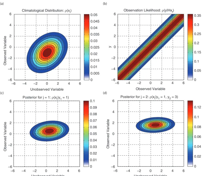
As alluded to in the beginning of this section, we construct here a simple data assimilation example that we believe will illustrate the basic properties of the more complex concepts in the remainder of this section in the simplest way. To this end, we assume the true states to be characterised by a two-vector whose climatological distribution is illustrated in Fig. 1a. This distribution is Gaussian with a variance of 3 on each variable and a covariance between the two variables of 1. Note that the setAtin this case is the entire plane as

a Gaussian vanishes nowhere. An observation of only one of the variables is made and defines an observation like-lihood with instrument error variance equal to 1 (Fig. 1b). Calculating eq. (2) from the climatological distribution and observation likelihood for an observation ofy11 obtains

the posterior in Fig. 1c. For simplicity, we further assume that the true model that is propagating the states forward in time is simply the identity. This implies that the posterior from eq. (2) is simply the prior for the next assimilation step in eq. (3) and the result of this calculation withy23

is plotted in Fig. 1d. One can see in Fig. 1c and 1d that the assimilation of the observations has reduced the vari-ance greatly for the observed variable but less so for the unobserved variable. In the next subsection, we will return to this example and illustrate its relationship to the forecast posterior.

2.2. The forecast posterior

Because of our fundamental inability to construct an exact model of the evolution of the general circulation of the atmosphere, the posterior distribution described by eq. (3) can never be produced by a data assimilation algorithm. This is true for several reasons. First, even if we could give

the forecast model the true state, it would not produce the correct forecast evolution because of incorrectly spe-cified parameters and altogether missing physics. Second, what exactly is the appropriate true state to give the fore-cast model as an initial condition is ambiguous given the fact that this model can only represent states that are ‘smoothed’, or said another way, truncated with respect to the truth (Frehlich, 2011). More on this notion will be presented in Sections 3 and 4.

Because the forecast model cannot represent the true attractor, we begin by defining the state on the forecast attractor,xf, as anM-vector and hypothesising that it too

is drawn from a ‘climatological’ distribution whose pdf we labelr(xf). We emphasise that the ‘climatology’ here is

different from that of the true distribution denoted above and results from running the forecast model for a very long

time, discretising state space, and counting the number of times the forecast state enters each cell of our discretisation. We again define from this forecast climatological distri-bution a new and distinct set of states Af with the

pro-perty that r(xf)0 and will subsequently refer to the set

Af as the ‘attracting manifold’ of the forecast model’s

representationof the physical system under consideration. Next, we hypothesise the existence of a map (function) over At0Af. We do this by relating the states on the

forecast attractor and the states on the true attractor through a vector-valued function:

xf ¼F xð Þt : (4)

The function, F, represents a mapping from the true attracting manifold to that of the forecast model. We emphasise that this is a mapping from one state space (At)

Unobserved Variable Observed Variable Climatological Distribution: ρ(x_t) −6 −4 −2 0 2 4 6 −6 −4 −2 0 2 4 6 0 0.005 0.01 0.015 0.02 0.025 0.03 0.035 0.04 0.045 0.05 Observed Variable y

Observation Likelihood: ρ(y|Hx_t)

−6 −4 −2 0 2 4 6 0 0.05 0.1 0.15 0.2 0.25 0.3 0.35 Posterior for j = 1: ρ(x_t|y₁ = 1) 0 0.01 0.02 0.03 0.04 0.05 0.06 0.07 0.08 0.09 0.1 Posterior for j = 2: ρ(x_t|y₁ = 1, y₂ = 3) 0 0.02 0.04 0.06 0.08 0.1 0.12 −6 −4 −2 0 2 4 6 Observed Variable −6 −4 −2 0 2 4 6 Unobserved Variable −6 −4 −2 0 2 4 6 Observed Variable −6 −4 −2 0 2 4 6 −6 Unobserved Variable −4 −2 0 2 4 6 (a) (b) (c) (d)

Fig. 1. Data assimilation on the high-resolution (true) attractor. (a) High-resolution climatological distribution, (b) high-resolution observation likelihood, (c) high-resolution posterior forj1 and (d) high-resolution posterior forj2.

to another (Af) and not a direct relationship between

today’s truth and today’s forecast, which because of the noise in the observations could not possibly satisfy eq. (4). We will assume that this function,F, has the property that for every xt in At there is a corresponding element of xf

in Af. However, we will not in general assume that the

converse is true and therefore we will discuss,F, as lacking an inverse, but we will also examine specific situations where this function does have an inverse. Please see Fig. 2. From a numerical weather prediction perspective, we view eq. (4) much like that of the algorithms in the ensemble post-processing and bias-correction literature (e.g. Glahn and Lowry, 1972; Raftery et al., 2005) in which climatolo-gical information is used to build relationships between forecasts and observations. Additionally, we view eq. (4) as having both a practical as well as a pedagogical application. From a practical perspective, one may wish to deduce the relationship [eq. (4)] from some climatological archive of forecast-truth pairs in order to implement the data assimila-tion algorithm discussed in this manuscript. By contrast, and from a pedagogic perspective, one may wish to simply assert a particular relationship in eq. (4) and subsequently use the framework presented below to understand its im-plications. This last tack will be the one illustrated in this manuscript as we will focus in Sections 3 and 4 on a linear map in eq. (4) that is to be interpreted as a smoothing operator as this was used in previous work in the represen-tation error literature (e.g. Liu and Rabier, 2002; Waller et al., 2013). In a sequel to this manuscript, we will illustrate estimation techniques forFand the results of its application to different cycling data assimilation experiments.

Equation (4) allows for the definition of several new densities in this problem that will prove to be useful tools in the subsequent analysis. Equation (4) implies that the

density that describes the distribution of states on the forecast attractor given a state on the true attractor, which we will refer to as aconversion density, is the Dirac delta function: q xf xt ¼d xfF xð Þt : (5)

This is because given a particular true statextthere is one

and only one forecast statexfthat it is related to and hence

there is no uncertainty in the position on the forecast attractor given a particular realisation of the state on the true attractor. It is important to realise that eq. (4) implies that while r(xfNxt) has zero variance that in general the

converseconversion densityr(xtNxf) has a non-zero variance

because Fdoes not necessarily have an inverse. Last, the assumption that the relationship between the two attractors is of the form [eq. (4)] allows for the subsequent simplifi-cation in eq. (5) that the conversion density is simply the Dirac delta function, but this assumption is technically not required by the following theory and is largely used to allow greater focus on the relationship between the lack of an inverse in eq. (4) and the representation error.

Bayes’ rule tells us that the two conversion densities discussed above can be related to each other through their associated climatological distributions as

q xf xt qð Þ ¼xt q xtjxf q xf : (6)

We may understand a little bit about the structure of the converse conversion densityr(xtNxf) by solving eq. (6):

q xtjxf ¼w xt;xf d xfF xð Þt ; (7) where w xt;xf ¼ qð Þxt q xf (8)

First, eq. (7) shows that whenFdoes not have an inverse, the densityr(xtNxf) is a weighted collection of Dirac delta

functions on the surface defined by fixing xf and

deter-mining the collection of statesxtfor whichF(xt)xf. Note

that becauseFonly produces states onAf we never need

evaluate w(xt,xf) for values of xf for which r(xf)0.

Second, as discussed in subsection 2.1, because the observa-tions in the data assimilation cycles from timesj1, 2,. . .,J

do not change the setAt, and the map [eq. (4)] is valid for

all At and Af, we may apply the map [eq. (4)], and its

corresponding conversion densities, to all data assimilation cycles,j.

To illustrate the properties of these conversion densities, we relate these densities to the two-vector example of subsection 2.1. Here, we define a forecast (low-resolution) state to be a scalar that arises from a smoothing operator that

ρ(xt)

At

Af ρ(xf)

Fig. 2. The attractors and their map. The two green squares represent the domain of the true states (large square) and the forecast states (small square). The region for whichqð Þxt >0 q xf >0

is denoted as the red (blue) shaded region. An example of the function in eq. (4) is denoted by the arrows, which travel from states inAt denoted by filled circles to states in Afdenoted by open circles. Note that multiple states inAtmay map to the same point inAf. We will show that this results in an error of representation.

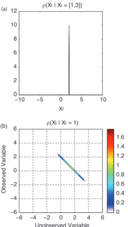
is an arithmetic mean:F¼½0:5 0:5. We use this operator in eq. (4) to define the forecast (scalar) states that are ob-tained from the high-resolution true (two-vector) states. Equation (5) is plotted in Fig. 3a for an example high-resolution state of xt¼½1 3

T

, which implies a low-resolution state ofxf2 becauseFxt2 in this case. Note

that the delta function in Fig. 3a is placed atxf2 and has

amplitude 10. The amplitude of 10 arises because we have defined integration numerically here as the trapezoidal rule. For the trapezoidal rule, the Dirac delta function is inversely proportional to the grid resolution that we are using to represent these densities. Here we have used a grid resolution of 0.1, which implies that the Dirac delta has amplitude 10. As described in the previous section, while

q x_fxt¼½1 3 T

is the Dirac delta function, the converse conversion densityr(xtNxf) is not. As an example, the

con-verse conversion density,r(xtNxf1), has non-zero

probabil-ity on a line defined byFxt1 weighted by the climatological

distributions throughwand is shown in Fig. 3b.

These conversion densities are useful because they allow one to convert between the true and forecast densities. For

example, the prior density on the attracting manifold of the forecast model is:

q xf YJ1 ¼ Z1 1 q xf xt qðxtjYJ1Þdxt: (9)

Equation (9) describes the distribution of forecastsxfthat

obtains from samplingr(xtNYJ1) for xt and using these

samples ofxtin eq. (4) to obtain samples ofxf. We may

apply eq. (9) to our simple example problem to find the prior distribution of forecasts for thej2 cycle (Fig. 4b). Recall that the prior distribution for our simple example problem is the previous (j1) posterior,r(xfNy11). Note

that the mode of this low-resolution prior is not the mode of either variable in the high-resolution prior. In fact, the mode of the low-resolution prior is the arithmetic mean of the mode of each resolution variable in the high-resolution prior. −10 −5 0 5 10 0 2 4 6 8 10 12 ρ (Xf | Xt = [1,3]) ρ(Xt | Xf = 1) Xf −6 −4 −2 0 2 4 6 −6 −4 −2 0 2 4 6 0 0.2 0.4 0.6 0.8 1 1.2 1.4 1.6 Observed Variable Unobserved Variable (a) (b)

Fig. 3. The conversion densities. (a) The conversion density de-scribing the distribution of forecast states given a state on the true attractor (xt¼½1 3

T

), and (b) the conversion density describing the distribution of true states given a state on the forecast attractor (xf1). −6 −4 −2 0 2 4 6 0 0.1 0.2 0.3 0.4 Low−Resolution Ob Likelihood −6 −4 −2 0 2 4 6 0 0.1 0.2 0.3 0.4 0.5 Low−Resolution Posterior Climatological Posterior (j=1) Posterior (j=2) xf y (a) (b)

Fig. 4. Data assimilation on the low-resolution (forecast) attractor. The low-resolution (a) observation likelihood and (b) climatological and posterior distributions forj1 and 2.

The conversion densities are central to our develop-ment because through them we are able to build one of the most important components of this work. These conversion densities allow us to show that the forecasts have their own posterior density defined as

q xf YJ ¼ Z1 1 q xf xt qðxtjYJÞdxt; (10)

which, upon using (3) and (5), implies

q xf YJ ¼C_Jq yJ xf q xf YJ1 ; (11)

wherer(yjNxf) is the conditional density for the observation

conditioned on the forecast state (which we shall refer to as theforecastobservation likelihood) andr(xfNYJ) represents

the density that describes the conditional distribution of forecast states given the entire observational record. This notion that the states on the forecast attractor have a posterior density that has been conditioned upon obser-vations of the state on a different attractor is a unique aspect of this work and will allow us to explicitly show how the difference in the two attractors leads to an error of representation.

Equation (11) shows that the data assimilation procedure, starting from the climatological distribution and proceeding forJassimilation steps, applies to the forecast model in so far as one simply replaces the true states,xt, with the

fore-cast states,xf, in eqs. (2) and (3) to define Bayesian data

assimilation on the forecast attractor. It is however im-portant to recognise that while eq. (11) looks superficially similar to eq. (3), it is in fact quite different. This is true for two reasons: (1) the data assimilation procedure for the forecast model begins with the forecast climatological distribution, which may be significantly different from the true climatological distribution, and (2) the forecast ob-servation likelihood is actually very different from the true observation likelihood. This difference between the true observation likelihood and the forecast observation likelihood will be described next.

2.3. The forecast observation likelihood

Central to understanding the forecast posterior distribution, and the manifestation of representation error within it, is the forecast observation likelihood. The observation likelihood in eq. (11) obtains from application of the chain rule of probability through the use of the conversion density as

q yJ xf ¼ Z1 1 q yJ xt q xtjxf dxt: (12)

An important difference between r(yJNxf) and r(yJNxt)

is that while the mean ofr(yJNxt) is the true state (Hxt)

and its variance is the instrument error, Ri, this is not

true of r(yJNxf). The mean of r(yJNxf) is, after use of

eq. (12): yf xf ¼ Z1 1 yJq yJ xf dyJ ¼Hxc; (13) xc xf ¼ Z1 1 xtq xtjxf dxt; (14)

where we will explicitly write this as a state-dependent bias (from the perspective of the forecast model attractor and its associated prior) as

yf xf ¼Hfxfþb; (15)

with this bias defined as

b¼HxcHfxf; (16)

andHf(pM) is the observation operator in the space of

the forecast model. At this point, we will leave the defini-tion and the distincdefini-tion betweenHandHf undefined. We

emphasise here however that the situation we will examine is one in which the difference betweenHandHfis because

Hfoperates on a truncated state vector and is not because

Hfhas been approximated or created in error. Nevertheless,

we will see subsequently that this difference between these two observation operators will turn out to be a central fea-ture of the analysis and therefore we shall return to discuss their differences at several points below.

Equations (13) and (14) show that the observation conditioned on the forecast is biased with respect to the truth (because the observation is of an object on the true attracting manifold and not on the forecast attracting manifold) and that bias is described by the mean of the conversion density. In addition, the variance about the mean state,yf(xf), is Rf xf ¼ Z1 1 yJyf yJyf T q yJ xf dyJ ¼RiþHPcH T ; (17) where Pc xf ¼ Z1 1 xtxc ð ÞðxtxcÞ T q xtjxf dxt; (18)

is the covariance matrix of the conversion density. Equa-tion (18) carries the informaEqua-tion that relates the forecast model states to the true attracting manifold. The term

HPcHTis the manifestation of the representation error in

the observation covariance matrix and shows that repre-sentation error occurs when the functionFdoes not have

an inverse. To see this note that when the functionFhas an inverse, thenw1 and

q xtjxf ¼d xf F xð Þt ¼d xtF 1 xf ; (19)

which clearly has a variance of zero and hence eq. (18) would vanish. Furthermore, note that if we use eq. (19) in eqs. (13) and (14), then we obtainyfHF1(xf), which is

biased from the perspective of the forecast attractor, where that bias isbHF1(xf)Hfxf. We may however remove

this bias by defining the observation operator in the space of the forecast model as HfHF

1

. This definition of the forecast observation operator is novel as it implies that we extend our view of what an observation operator does. The observation operator, HfHF1, implies that the

forecast observation operator should include a ‘bias’ correction for the particular forecast model that we are using. In Section 4, this definition of the forecast observa-tion operator will be generalised to linear equaobserva-tions [eq. (4)] that do not contain an explicit inverse and subsequently shown to be the proper way to account for representation error. In the meantime, however, we will maintain the general form forHfthat we have been using thus far.

In order to understand the forecast observation like-lihood better, we apply our example problem to eq. (12) to find the resolution observation likelihood. This low-resolution observation likelihood is plotted in Fig. 4a as a function of observation and conditioned on the low-resolution state of xf1. Because the observation is

actually of the high-resolution state, the low-resolution observation likelihood is biased (with respect to the low-resolution states), which can be seen by the mode of the distribution not being centred on the low-resolution state ofxf1. It is actually centred atxf1/2, where this bias

may be seen as coming from the bias in the forecast climatological distribution whose mean is at xf ¼ 1=2.

The forecast observation likelihood has a variance of 2, of which 1/2 of this variance (recall that the instrument error is 1) can be attributed to representation error and eq. (18). Finally, the low-resolution posterior [eqs. (10) and (11)] for the observation j1 and 2 cycles is plotted in Fig. 4b. The posterior for thej1 cycle has its mode at 1/2, and the mode of the posterior for thej2 cycle is at 1.2. Again, the mode at each cycle is located at the arithmetic mean of the location of the modes in the true (high-resolution) posteriors.

2.4. Data assimilation

Because we are interested in doing data assimilation with these concepts, we will now derive the minimum error var-iance estimate of a linear estimator on the forecast models attractor, which, in this context, is the Kalman filter

(Kalman, 1960) for the states on the forecast attractor. This formula is derived by minimising the trace of the

expected posterior forecast covariance matrix about a linear estimator. The expected posterior forecast covariance matrix may be written as:

Pa¼ Z1 1 Z1 1 xfxa xfxa T q xf YJ dxfq yJ YJ1 dyJ; (20)

where the analysis update equation, whose ‘error’ variance is being measured, takes the form of a linear estimation equation xa¼xfþG v½ h iv; (21) where xf ¼ Z1 1 xfq xf YJ1 dxf ¼ Z1 1 F xð Þt qðxtjYJ1Þdxt:(22)

The overbar onPa in eq. (20) is there to make clear that

this is the expression for the expected posterior covari-ance matrix as it has been averaged over all the obser-vations [see Hodyss and Campbell (2013) for further discussion]. The innovation in eq. (21) is v¼yJHfxf,

which we emphasise uses the observation operator in the space of the forecast model. The expected innovation,h iv, in eq. (21) is there because the observations with respect to the forecasts are biased because the observations are taken on the true attracting manifold. This de-biasing of the innovation in eq. (21) is critical to get the data assimilation to put the analysis at the centre ofr(xfNYJ)

and therefore the posterior distribution on the desired forecast attractor.

It is important to realise that while the quantities derived in eqs. (13) and (14) through eq. (17) are interesting descriptions of the corresponding densities, they are in fact not the ones that would be used in a data assimila-tion algorithm. This is because as shown in eq. (20) those expressions need to be averaged over the forecasts in the derivation of the update equations. This averaging for eqs. (13) and (14) would take the form:

yf ¼ Z1 1 yf xf q xf YJ1 dxf ¼Hfxfþb; (23) whereb¼h i ¼v HxtHfxf and xt¼ Z1 1 xtqðxtjYJ1Þdxt: (24)

In addition, the observation error variance that would be used in a data assimilation algorithm is obtained from

Rf ¼ Z1 1 Rf xf q xf YJ1 dxf: (25)

Note that the result of the integration in eq. (25) is an observation error variance that is not state-dependent. The derivation of the Kalman gain requires the use of an observation error covariance matrix that is the result of a weighted average over all possible observation error covar-iance matrices and therefore cannot depend on the state.

Equation (25) is interesting because we may use eq. (17) in eq. (25) to obtain: Rf ¼Riþ Z1 1 HPcH T_{q x} f YJ1 dxf; (26) where Z1 1 HPcH T_{q x} f YJ1 dxf¼HPtH T_H fPfH T f HfPfb PT fbH T f Pbb; (27) Pt¼ Z1 1 xtxt ð ÞðxtxtÞ T qðxtjYJ1Þdxt; (28) Pf ¼ Z1 1 xfxf xf xf T q xf YJ1 dxf; (29) Pfb¼ Z1 1 xf xf bb T q xf YJ1 dxf; (30) Pbb¼ Z1 1 bb bb T q xf YJ1 dxf: (31)

Equation (27) shows that representation error is the difference between the true covariance, the covariance of the forecasts and the bias, and the covariance matrix of the state-dependent bias all mapped to observation space.

The steps required to perform the minimisation of the trace of eq. (20) are well known, can be found in Hodyss (2011) and will not be repeated here. The result of this minimisation is that thegain matrix,G, can be written in two equivalent ways:

G1¼PftH T _HP tH T_þR i 1 ; (32) G2¼ PfH T f þPfb h i HfPfH T f þHfPfbþP T fbH T f þPbbþRf h i1 ; (33) where Pft¼ Z1 1 F xð Þ t xf xtxt ð ÞTqðxtjYJ1Þdxt; (34) PftHT¼PfHTf þPfb: (35)

The first gain matrix,G1, uses information from the true

attractor that is subsequently mapped back to the forecast attractor through the covariance between the states on the two attractors,Pft. This version of the gain is most similar

to the traditional Kalman gain whereby the numerator relates the (true attractor’s) observation space to the state space to be updated (forecast attractor) using the covar-iance [eq. (34)]. This version of the gain matrix is of course impossible to implement in practice as it requires use of the true prior distribution.

The second gain matrix,G2, is novel and only uses the

information on the forecast model attractor along with the function Fto infer the relationship between the true and the forecast attractors. This second gain matrix has two terms in its numerator. The first term is the standard term that maps the observation space to the state space to be updated, but totally from within the forecast attractor. The second term is new and accounts for the possibility that on the forecast attractor there is no covariance between the observation space and state space to be updated but, because the observation is actually of a state on the true attractor and there may be a covariance between the true attractor and the forecast state space to be updated, there should in fact be a correction at that location. This new term is shown in eq. (35) to be precisely the difference between the forecast state-space/true observation-space covariance (PftHT) and the forecast state-space/forecast

observation-space covariance (PfHTf). Equation (35) shows that the

numerators of eqs. (32) and (33) would be identical if the forecast-bias covariance matrix,Pfb, would vanish. In

Section 4, we show how to choose the forecast observation operator to eliminate this forecast-bias covariance matrix.

Last, it is important to realise that the gain matrices [eqs. (32) and (33)] when used in eq. (21) do not in fact provide an estimate of the true state on the true attractor. The gain matrices [eqs. (32) and (33)] when used in eq. (21) find the state estimate that is closest (in the sense of the function

F and in mean-square) to theforecast that obtains from mapping the truth through eq. (4). Hence, the gain matrices [eqs. (32) and (33)] push the state estimate from the true attracting manifold onto the forecast attracting manifold and is actually likely to push the state estimate further from the observations than it would have been if we had not altered the numerator and denominator of the gain matrix to account for this error in representation. The benefit from using these new gain matrices is therefore

not their distance from the true attractor but actually the fact that they produce a state estimate near to the fore-cast attractor, which is likely to produce a better, and more balanced, forecast.

3. Smoothing operators

Previous work in the representation error literature has examined the situation where the relationship between the states being observed by the observational instruments and that produced by the forecast model are related by a smoothing operator (e.g. Mitchell and Daley, 1997a, 1997b; Liu and Rabier, 2002; Waller et al., 2013). Following this work, we will assume that the forecast model resolution is coarse as compared to the true model resolution, that is,

MBN. In addition, we will assume the functionFis linear, but we make no assumptions on the shape of the prior distributions on either attractor.

The function F will be assumed to be a linear matrix operator that acts to ‘smooth’ the true state to the resolution of the forecast model, viz.

xf¼Sxt; (36)

whereSis anMN matrix whose singular value decom-position results in

S¼UK1=2 0VT; (37)

with the left singular vectors contained inU(MM), right singular vectors in V (NN), L(MM) the diagonal matrix of singular values and 0 [M(NM)] the zero matrix. The bracket in eq. (37) is a truncation operator, and along withL, which we assume to be either constant (white) or steeply sloped (red), we view as a ‘smoothing’ operator. We attach to this notion of ‘smoothing’ the philosophy prevalent in numerical modelling (e.g. Lilly, 2005) in which forecast model output is assumed to represent grid-cell averages of the true state around each nodal point of the model’s grid representation of the spatial domain. Note that the statement [eq. (36)] states that the only difference between the forecast and the truth is through the smoothing of that state, which ignores the fact that a truncated model will differ in its cascades of energy and enstrophy (i.e. the nonlinear interaction be-tween scales and their subsequent evolution).

Because S isMN and MBN, the matrix Swill not generally have an inverse. This has important implications for the structure ofr(xtNxf) as it implies that there exists

a hyperplane defined by all of the states,xt, that satisfy

eq. (36) for a given forecast state xf. Along this plane,

r(xtNxf) has zero probability, and this results in a

non-zero variance of the converse conversion density, which as shown in eq. (18) leads to the error of representation.

An explicit example ofr(xtNxf) that had non-zero variance

was presented in Fig. 3, and in this case one could see in that figure that the hyperplane alluded to above was reduced to a line in the two-dimensional plane ofxt.

The smoothing operator in eq. (37) will lead to a bias in the observation mean [eq. (23)]. This bias leads to the expected innovation being

v

h i ¼b¼ HHfS

xt: (38)

The bias results from the difference between the true prior mean and the ‘smoothed’ one obtained after use of eq. (36). Similarly, the use of eq. (36) in thegain matrix,G[eqs. (32) and (33)], obtains: G1¼SPtH T HPtH T_þ Ri 1 ¼SGt; (39) G2¼ PfH T f þPfb h i HfPfH T f þR f h i1 ; (40)

wherePtis the covariance matrix of the true prior,

Pf ¼SPtS T ; (41) Pfb¼SPt HHfS T ; (42) Rf¼Riþ HHfS Pt HHfS T Pbb; (43) Rf¼HfPfbþP T fbH T f þPbbþRf ¼RiþHPtH T HfPfH T f: (44)

In eq. (39), the gain matrixGt, which is the true gain matrix

for the true attractor, is mapped into the forecast space through application of the smoothing matrix S. In eq. (40), the gain matrix is calculated using only quantities known from the forecast distributions and the matrixS. The quantityRf is an abstraction of the observation error

covariance matrix to include all the terms except the forecast covariance matrix in observation space in the denominator of eq. (40). We will refer to this quantity as the effective

observation error covariance matrix. The effective obser-vation error covariance matrix reduces to the sum of the instrument error and the difference between the true and forecast covariance matrices in observation space. Note that the difference between the effective observation covar-iance matrix, Rf, and the actual observation covariance

matrix,Rf, is entirely a result of the matricesPfbandPbb.

Given eqs. (36) and (37), it may be shown that thetrace

(Pt/N)]trace(Pf/M), and therefore the diagonal of R

f is

equal to or greater than the instrument error,Ri. This fact

about smoothing matrices of the form [eq. (37)] implies that high-resolution models should as a general rule have greater variance than low-resolution models.

This matrix Rf is important because it makes the

con-nection between the Kalman gains G1 andG2. The gain

gain matrix in eq. (40). This implies that the innovation variance in the denominator, as calculated both ways, must be equal, viz. HfPfH T f þR f ¼HPtH T_þ Ri: (45)

This relationship may be proven by using eq. (44) in eq. (45). This shows that if we define the error of represen-tation as a property of the covariance matrix of the fore-cast observation likelihood, then one cannot actually deduce it straightforwardly from the innovation variance (e.g. Hollingsworth and Lo¨nnberg, 1986; Desroziers et al., 2006). The object that can be deduced directly from the innovation variance isRf and notRf. More discussion of

the differences between Rf and Rf will be presented in

Section 4.

4. Gaussian statistics

In this section, we add to the development of Section 3 the assumption of Gaussianity to the climatological distribu-tions and linearity in the true and forecast model evolution equations. This implies that the prior distributions of both the forecast and true systems must also be Gaussian. It is important to point out that the assumption of Gaussian error statistics in the climatological distributions and linear error evolution implies that the setsAtandAfare no longer

bounded in state space as is implied by Fig. 2 but now extend to include all possible states in their domain.

4.1. Theory

A simple way to construct a Gaussian problem that is amenable to analysis is through the use of a discrete Fourier series representation. To this end, we assert a Gaussian covariance model for the true (high-resolution) states of the form

xt¼xtþZg; (46)

wherext is anN-vector, Zis the square-root of the true

covariance matrix,

Pt¼ZZ T

; (47)

and h is an N-vector of random numbers drawn from

N(0,I). We construct eq. (47) using a sinusoidal basis in which the columns ofE(NN) contain the sinusoids such that

Pt¼ECE

T_{; (48)}

Gis a diagonal matrix whoseith element of the diagonal is defined fromCi¼aea

2_k2

i,k_iis the wavenumber associated

with theith basis function ofE, anda¼N P N i¼1

ea2_k2

i. The

parameter a determines the slope of the true spectrum,

where largeais associated with a red spectrum and small

ais associated with a white spectrum.

We connect the true (high-resolution) states to the forecast (low-resolution) states through a smoother that operates as:

S¼EL D1=2T 0

ET; (49)

where D (MM) is a diagonal matrix whose diagonal elements ared_i¼eb2_k2

i,E_L(MM) is the low-resolution

basis whose columns are also the sinusoids andT(MM) is a diagonal matrix with the valuepffiffiffiffiffiffiffiffiffiffiffiffiM=Nalong the diagonal. The matrixDrepresents the climatological ‘model error’ on the resolved scales and would be equal to the identity matrix if the forecast model’s climate at the resolved scales was identical to the true model’s climate at those same scales. The matrix implied by the bracket in eq. (49) performs a truncation of the high-resolution basis to theM-dimensional subspace, while the matrix T assures that the Fourier coefficients calculated from the high-resolution basis are reweighted consistently with respect to the low-resolution basis.

Equation (49) allows for the creation of the low-resolution forecast states from the true states in eq. (46) using eq. (36). This implies that the forecast error covariance matrix may be written as Pf ¼SPtS T_¼ EL D1=2T 0 CD1=2T 0TETL: (50)

Because G are the true (high-resolution) eigenvalues, eq. (50) shows that the forecast covariance matrix would be correct up to its M eigenvalues if the climatological model error D could be removed. We show next how to remove this climatological model error by accounting for the error of representation.

Because the true states and the forecast states are Gaussian and their relationship is described by a linear operator, we know that the mean of the converse conversion density

q xtjxf

h i

is a linear function of the vector it is conditioned upon. This presents us with a direct method to calculate the prediction of the observation by the forecast state:

yf xf ¼Hxc¼HxtþHGp xfxf

h i

; (51)

where

Gp¼Z SZ½ y¼Sy: (52)

The superscript $in eq. (52) denotes the Moore-Penrose inverse (Golub and Van Loan, 1996). The pseudo-inverse is constructed by finding the singular value decom-position, viz.

SZ¼EL D1=2T 0

and then noting that its pseudo-inverse is therefore SZ ½ y¼EC1=2 D1=2_T1 ₀ T ET L: (54)

Equation (54) is thepseudo-inverse of eq. (53) in the sense that SZ[SZ]$rr but ½SZySZq6¼qfor arbitrary vectors

r andq. Please see Appendix A for a brief derivation of eq. (51). It is important to note in eq. (52) that the matrix

Zis cancelled by the pseudo-inverse operation such that the only information required to determineGpis the

smooth-ing matrix [eq. (49)]. In practice, one would build eq. (49) by estimating its components using an archive of truth-forecast pairs as is done in bias-correction algorithms (Glahn and Lowry, 1972). Moreover, this implies that we may view eq. (51) as simply a bias-correction algorithm that we build into the data assimilation system to account for the fact that the forecast model’s estimate of the observation is, in effect, biased.

Equation (51) is remarkable in so far as this construc-tion allows us to calculate the important quantities from Sections 2 and 3 without the need to explicitly develop the conversion densities. For example, the representation error is therefore:

RfRi¼HEHE T

HT_{; (55)}

whereUis a diagonal matrix with the value of the diagonal ofUsatisfying:

H_i¼ 0; i¼1; :::;M

C_i; i¼Mþ1; :::;N

: (56)

The term on the right-hand side of eq. (55) arises from eq. (43). This term clearly shows that the representation error [eq. (55)] is simply the portion of the high-resolution spectrum that is missing from the forecast states. Note that forMN, and therefore no truncation, the elements ofU vanish and there is no representation error. This is again a result of there being, in that case, an inverse available whenMN and, as discussed in Section 2, this implies that the representation error must vanish. This point is important because it shows that the climatological model error on the resolved scales (D) is irrelevant to both the existence of representation error and to the structure of the representation error. By contrast, eq. (44) for which we are interested inRfRidoes depend on the climatological

model error on the resolved scales (D) through eq. (50). An important quantity in our development of Section 2 was the state-dependent bias of the forecast model’s estimate of the observation [eq. (16)], b, which given eq. (51), implies: b¼ HSy Hf h i xf þH xtSyxf h i : (57)

The first term in eq. (57) is interesting because it corresponds to the mismatch between the forecast model’s estimate of the true observation operator HS$ in eq. (51) and the observation operator we are actually usingHf. We

empha-sise here that this mismatch is not one in which we are implying thatHfis incorrect in the sense that if, for example,

we had a point measurement that there would be some form of inaccuracy in the interpolation to the observation location. Indeed, even in this case of a point measurement, in which we are assuming we have a perfect interpolation, the mismatch inferred by eq. (57) is between the statistically derived observation operatorHS$, which now corresponds to more than just an interpolation, and the operator,Hf.

Equation (57) suggests that if we defineHfsuch that,

Hf HSy; (58)

we may remove this state-dependent bias term, which subsequently renders Pfb0 and Pbb0. This implies

that in this data assimilation system the observation operator doesnotsimply map the truth to the observation, but rather it maps the forecast to the observation and, because the forecast is in a different portion of state space than the truth, this requires the matrix operator, HS$

rather than justH.

One of the most important results of choosing eq. (58), and subsequently rendering Pfb0 and Pbb0, is that

this results inRf ¼Rf, and therefore the choice [eq. (58)]

has removed the impact of the climatological model error on the resolved scales,D, in the forecast covariance matrix and therefore also in Rf. This has two important

con-sequences: (1) innovation-based techniques (e.g. Hollings-worth and Lo¨nnberg, 1986; Desroziers et al., 2006) for the estimation of Rf are therefore self-consistent estimators

of the representation erroronly when the choice (58) has been implemented and (2) as we show next this provides a direct way to remove the deleterious impact of the climatological model error on the state estimate from the data assimilation algorithm.

Subsequently, by employing eq. (58), it can be shown that the gain matrix written in terms of the forecast quantities [eq. (40)] is now:

G2¼PfSy T_HT _HSy_P fSy T_HT_þR f h i1 : (59)

This new gain matrix is the most important result of this manuscript. The calculation of the operatorGphas allowed

for the creation of a new observation operator HS$ that represents the forecast model’s estimate of the observation of states on the true attractor. Subsequently, this has allowed the calculation of the correctnumeratorin eq. (59) that represents the covariance between the states on the

forecast attractor and the observations of the true attrac-tor. Equation (58) results in

HfPfH T f ¼HSyPfSy T HT¼HE CM 0 0 0 ETHT; (60) v h i ¼HE 0 0 0 I ETxt; (61)

whereGMdenotes the firstMeigenvalues ofG,and0is the

zero matrix. Equation (60) shows that the choice [eq. (58)] results inHfPfH

T

f being correct up to the resolution of the

forecast model in the sense that the climatological model error denoted by D has been removed. Equation (51), which describes the bias in the innovation owing to the unresolved scales of motion, is a result of the scales in the true prior mean that are missing in the forecast prior mean.

4.2. Spatially extended example

We now explore the theory discussed above for the spatially extended problem described in this section by employing some simple example problems. We will not re-define the observation operator in order to clearly show the differences between RfRi and R

f Ri, which will

underscore the importance of applying eq. (58), as it was already proven above to remove this difference. We will defineHto be the operator that observes each point of the low-resolution (forecast) state. Hence, in these experiments,

Hfwill simply be the identity operator for the point

mea-surements we have available. We emphasise again that employing eq. (58) would lead to an observation operator for these point measurements that is not the identity operator even though these are point measurements, which as we have proven above corrects the problems to be

0 1 2 3 4 5 6 −0.1 0 0.1 0.2 0.3 0.4 0.5 0.6 0.7 0.8 0.9 0 1 2 3 4 5 6 −0.02 −0.01 0 0.01 0.02 0.03 0.04 0.05 0.06 0.07 1.0 (a) (b) x 0 1 2 3 4 5 6 −0.1 −0.05 0 0.05 0.1 0.15 0.2 0.25 0.3 0.35 0.4 0 1 2 3 4 5 6 −0.1 0 0.1 0.2 0.3 0.4 0.5 0.6 0.7 x (c) (d) True M = 16 M = 8 M = 16 M = 8 R_f−R i R* f−Ri Pbb − − R_f−R_i R* f−Ri Pbb − −

Fig. 5. Pure spectral truncation. (a) Three one-point prior covariance functions: blue is the high-resolution (true) covariance model, red is theM16 low-resolution (forecast) covariance model and green is theM8 low-resolution (forecast) covariance model. (b) One column of the smoother matrix [eq. (62)] forM16 (red) andM8 (green). (c, d) The main components of the theory forM16 and

M8, respectively: blue is the representation error covariance (RfRi), red is theeffectiverepresentation error covariance (R

fRi) and

illustrated next. In order to maintain a connection with previous work (e.g. Mitchell and Daley, 1997a, 1997b; Liu and Rabier, 2002; Waller et al., 2013), we begin by defining the low-resolution (forecast) states as obtained from a smoother that operates as a pure spectral truncation such that we setb0 in eq. (49), which obtainsDIand

S¼EL½T 0E T

: (62)

We seta1/12 and plot the central column ofPtin Fig. 5a,

which represents the one-point covariance function for the point xp. The length of the state vector for the high-resolution (true) states will beN256. In Fig. 5a, we also plot the central column ofPffor two different truncation

matricesS: one is forM16 and the other is forM8. Fig. 5b shows the corresponding central column of S, which maps the high-resolution (true) states to the low-resolution (forecast) states. The smoothing functions in Fig. 5b show that truncating the true spectrum results in smoothing kernels that average the true state globally to produce the local low-resolution (forecast) state. In addi-tion, note that the smoothing kernel weights the true state both positively and negatively, which we will see shortly results in long distance negative correlations. Figure 5c and 5d shows the one-point covariance function (again for the central column) for Rf Ri and R

fRi for the M16

andM8 cases. In both cases, the representation error

RfRi and the effective representation errorR

fRi are

very nearly equal in the centre of the domain but differ in the far-field. We will show by contrast below that this equality between these two matrices is due to the pure truncation in this case. When we invoke a Gaussian smoother (i.e. D"I), which as noted above corresponds to a climatological model error on the resolved scales,Rf

Ri andR

fRi will become substantially different. Also,

note that there exists a strong far-field positivenegative wave pattern inRfRiand less so forR

fRi. This is due

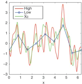
to the aforementioned positivenegative weightings in the smoothing kernels of Fig. 5b. An example of a randomly constructed high-resolution (true) state [eq. (46)] is shown in Fig. 6. Using eq. (62), we may produce the correspond-ing low-resolution (forecast) state from theM8 forecast state shown in Fig. 6. Also, shown in Fig. 6 is the estimate of the true state,xc, given the low-resolution forecast state

from eq. (51) using theM8 forecast state shown in that figure. This ‘best estimate’ from eq. (51) makes use of the linear regression in eq. (51) but does not make use of the observation operator,H. In this sense, this ‘best estimate’ is simply a state-dependent bias correction of the forecast.

The next set of experiments will make use of the matrix

D. Here, we study eq. (49) for b1/6, which implies a Gaussian smoother on the degrees of freedom that are retainedaftertruncation. The same true covariance model

is used in this experiment, Pt, for which the one-point

covariance function is repeated in Fig. 7a. Again, in Fig. 7a, we also plot the central column of Pf for two different

truncation matrices T: one is for M256 and the other is forM16. Note that theM256 case corresponds to no truncation at all as the forecast state vector and the true state vector are equal (MN256). The M256 case provides an example of a forecast model error that does not arise from a reduction (truncation) of the number of degrees of freedom in the forecast model. The smooth-ing kernels for these two cases are shown in Fig. 7b. The truncated smoothing kernel (M16) shows the positive

negative oscillations in the far-field that we saw previously. Contrast this with the non-truncated smoothing kernel (M256) that is completely local.

The application of these smoothing kernels produces distinctly different responses in Rf Ri and R

fRi.

For the M256 case, the S is full-rank, has an inverse and results inRf Ri¼0as shown in Fig. 7c. However,

because the smoothing matrixSstill produces a difference betweenPtandPf, which implies thatR

f Ri is non-zero

as shown in Fig. 7c. Hence, when the forecast model is full-rank, but fails to reproduce the climatology of the true attractor, the representation error nonetheless vanishes. This type of climatological error in the model must still be accounted for usingRfRi andGp. In the case where

M16, which implies both a Gaussian smoothing and a truncation, one can see in Fig. 7d that both representa-tion error and RfRi are non-zero and quite different.

This difference between Rf Ri and R

f Ri illustrates

that one can only estimate the representation error from

0 1 2 3 4 5 6 −3 −2 −1 0 1 2 3 4 High Low Xc x _

Fig. 6. Example high-resolution state, low-resolution state (M8) and mean of the conversion density, which is labelled above as the ‘best estimate’. The low-resolution state is defined only at the grid-points denoted by the open circles.

innovation statistics when eq. (58) is implemented because this is the only way to renderPfb0andPbb0.

5. Summary and conclusions

A framework has been presented to understand the origin of the representation error as well as to properly frame attempts at estimating and accounting for its effects. We have extended the work of Kalman (1960), whose data assimilation algorithm is optimal for Gaussian systems for which the flaws in the model were accounted for using a white noise forcing, to the case where the observations are of states on a true ‘attractor’ and the model evolution produces states on a forecast ‘attractor’ with both states Gaussian distributed and a linear map existing between them, but with no applied white noise forcing. In practical terms, when the distributions are not Gaussian and the

mapping between the two attractors is not linear, we have derived the best linear, unbiased estimation technique. For this case, we have shown that in this data assimilation algorithm the observation operator does notsimply map the truth to the observation, but rather it maps the forecast to the observation, and because the forecast is in a different portion of state space than the truth, this requires a modified observation operator. We emphasise that the operation of this new data assimilation framework only requires the prior distribution on the forecast model attractor and the functionF, and does not need the prior distribution on the true attractor, to correctly assimilate observations of states on the true attractor. We view this map in eq. (4) much like that of the algorithms in the ensemble post-processing and bias-correction literature (e.g. Glahn and Lowry, 1972; Raftery et al., 2005) in which climatological information is used to build relationships

0 1 2 3 4 5 6 −0.1 0 0.1 0.2 0.3 0.4 0.5 0.6 0.7 0.8 0.9 0 1 2 3 4 5 6 −0.2 −0.1 0 0.1 0.2 0.3 0.4 0.5 0.6 0.7 R–_f−R_i –* R_f−R_i Pbb 1.0 (a) (c) True M = 256 M = 16 0 1 2 3 4 5 6 −0.02 −0.01 0 0.01 0.02 0.03 0.04 0.05 0.06 0.07 R–_f−R_i –* R_f−R_i P_bb 0 1 2 3 4 5 6 −0.2 −0.1 0 0.1 0.2 0.3 0.4 0.5 0.6 (b) (d) M = 256 M = 16

Fig. 7. Gaussian Smoothing. (a) Three one-point prior covariance functions: blue is the high-resolution (true) covariance model, red is theM256 low-resolution (forecast) covariance model and green is theM16 low-resolution (forecast) covariance model. (b) One column of the smoother matrix forM256 (red) andM16 (green). (c, d)The main components of the theory forM256 andM16, respectively: blue is the representation error covariance (RfRi), red is theeffectiverepresentation error covariance (R

fRi) and green is

between forecasts and observations. As such, this new framework has shown how to properly include the in-formation normally obtained from ‘bias-correction’ algo-rithms within the data assimilation system.

As discussed in the introduction, the notion that the true state might not be the best initial condition for the flawed forecast model has led us to choose to develop a data assimilation system that attempts to produce a state estimate on the forecast attractor. This obviously produces a state estimate that may not be as close to the truth as is required in some applications. Note however that we may use the state estimation procedure described in Appendix A to map our forecast back to the true attractor in order to produce a state estimate on the true attractor. This of course is nothing more than the well-known post-processing of a forecast but using the infrastructure that we have already developed for the data assimilation algorithm.

In any event, this new framework shows that the re-presentation error arises from the lack of an inverse in the relationship between the true attracting manifold and that of the forecast models. This lack of an inverse in their relationship results when the forecast model is a truncated representation of the true states. In other words, represen-tation error does not occur when the forecast model is simply in error in its representation of climatology. The error that the model must make for representation error to exist is one in which the forecast model has been truncated to represent fewer degrees of freedom than the number of degrees of freedom describing the true states. In this specific case, the forecast observation likelihood

q yJ

xf

h i

will have a variance greater than that of the error of the instrument and is also likely to have a cor-relation between observations. In the Gaussian case, it was shown explicitly that this inflation and correlation structure arises as the covariance matrix of the portion of the true spectrum that goes missing from the truncated forecast model. Lastly, it was shown that innovation-based techni-ques (e.g. Hollingsworth and Lo¨nnberg, 1986; Desroziers et al., 2006) for the estimation of representation error covariance matrices are self-consistent estimators of the representation erroronly when the observation operator has been modified to account for the attractor differences.

Applying this new framework to specific problems in the geosciences will require estimation of the map between the true attractor and that of the forecast model [eq. (4)]. We imagine a proxy for such a model could be developed from the difference between high-resolution and low-resolution simulations. After development of the map [eq. (4)], one must develop the observation gain (Gp) for

each observation in which one is interested in accounting for errors in representation. We suggest performing this step using an observation-by-observation approach as this will likely lead to a reduction in the size of the matrices in the

calculation [eq. (52)]. Research into performing this estima-tion ofSis underway and will be reported in a sequel.

6. Acknowledgements

We gratefully acknowledge support from the Chief of Naval Research PE-0601153N and from the NERC National Centre for Earth Observation in the UK and the European Space Agency. We thank Jeff Anderson for a thorough reading and insightful comments on this work.

7. Appendix

The Moore-Penrose Inverse and the Minimum Variance Estimate

We begin with eq. (36) and decompose it into prior mean and perturbation:

xf ¼Sxt;eef ¼Seet (A1a,b)

whereeef ¼xfxf andeet¼xtxt. Equation (46) tells us

that

eet¼Zgg (A2)

where h is a N-vector whose elements are drawn from

N(0,1). Therefore, we attempt to minimise the cost function

Jð Þ ¼gg 1 2 eefSZgg h iT ee_fSZgg h i (A3)

to find that the minimum of eq. (A3) is defined by an infinite number of solutions of the form:

^ g g¼½SZyeef þE2nn (A4) where SZ ½ y¼EC1=2 D1=2_T1 ₀ ET L (A5) E¼½E1 E2 (A6)

and j is a vector of length (N-M) that is composed of random noise with the property that it is a random draw from N(0,GNM) with GNM denoting the last (N-M)

elements of the diagonal of G. In eq. (A6), E has been subdivided such that we defineE1as the firstMcolumns of E and then place the remaining columns into E2. We

choose the best solution from the set [eq. (A4)] by requiring the solution at the minimum of eq. (A3) to also minimise

eeT tP

1

t eet, which may be shown to imply thath

T

h is also a minimum. The addition of this constraint chooses j0, which then defines the solution as

^

eet¼Z SZ½ yeef (A7)

Equation (A7) defines the minimum variance estimate ot

under the constraint thateeT tP

1

eq. (A7) finds the minimum variance estimate of eq. (A1a,b) for the stateotgivenof. The minimum variance estimate of

a linear estimator will be equal to the mean of the conversion density when that density is Gaussian. When that density is not Gaussian, it then reduces to the bestlinear, unbiased estimate of the mean of the conversion density.

References

Daley, R. 1993. Estimating observation error statistics for atmo-spheric data assimilation.Ann. Geophys.11, 634647. Desroziers, G., Berre, L., Chapnik, B. and Poli, P. 2006. Diagnosis

of observation, background and analysis-error statistics in observation space.Q. J. Roy. Meteorol. Soc.126, 33853396. Frehlich, R. 2006. Adaptive data assimilation including the effect

of spatial variations in observation error.Q. J. Roy. Meteorol. Soc.132, 12251257.

Frehlich, R. 2008. Atmospheric turbulence component of the innovation covariance.Q. J. Roy. Meteorol. Soc.134, 931940. Frehlich, R. 2011. The definition of ‘truth’ for numerical weather prediction error statistics.Q. J. Roy. Meteorol. Soc.137, 8498. Glahn, H. R. and Lowry, D. A. 1972. The use of model out-put statistics (MOS) in objective weather forecasting.J. Appl. Meteorol.11, 12031211.

Golub, G. and Van Loan, C. F. 1996.Matrix Computations. The Johns Hopkins University Press, Balitmore, MD, USA, 687 pp. Hodyss, D. 2011. Ensemble state estimation for nonlinear systems using polynomial expansions in the innovation.Mon. Weather Rev.139, 35713588.

Hodyss, D. and Campbell, W. F. 2013. Square root and perturbed observation ensemble generation techniques in Kalman and quadratic ensemble filtering algorithms.Mon. Weather Rev.141, 25612573.

Hodyss, D., McLay, J. G., Moskaitis, J. and Serra, E. A. 2014. Inducing tropical cyclones to undergo Brownian motion: a comparison between Itoˆ and Stratonovich in a numerical weather prediction model.Mon. Weather Rev.142, 19821996.

Hollingsworth, A. and Lo¨nnberg, P. 1986. The statistical structure of short-range forecast errors as determined from radiosonde data. Part I: The wind field.Tellus A.38, 111136.

Janjic, T. and Cohn, S. E. 2006. Treatment of observation error due to unresolved scales in atmospheric data assimilation.Mon. Weather Rev.134, 29002915.

Kalman, R. E. 1960. A new approach to linear filtering and prediction problems.J. Basic. Eng.82, 3545.

Lilly, D. K. 1962. On the simulation of buoyant convection.Tellus.

14, 148172.

Liu, Z.-Q. and Rabier, F. 2002. The interaction between model resolution, observation resolution and observation density in data assimilation: a one-dimensional study.Q. J. Roy. Meteorol. Soc.128, 13671386.

Mitchell, H. L. and Daley, R. 1997a. Discretization error and signal/error correlation in atmospheric data assimilation (I). All scales resolved.Tellus A.49, 3253.

Mitchell, H. L. and Daley, R. 1997b. Discretization error and signal/error correlation in atmospheric data assimilation (II). The effect of unresolved scales.Tellus A.49, 5473.

Oke, P. R. and Sakov, P. 2008. Representation error of oceanic observations for data assimilation.J. Atmos. Oceanic Technol.

25, 10041017.

Petersen, D. P. and Middleton, D. 1963. On representative observations.Tellus A.15, 387405.

Raftery, A. E., Gneiting, T., Balabdaoui, F. and Polakowski, M. 2005. Using Bayesian model averaging to calibrate forecast ensembles.Mon. Wea. Rev.133, 11551174.

Richman, J. G., Miller, R. N. and Spitz, Y. H. 2005. Error estimates for assimilation of satellite sea surface temperature data I ocean climate models.J. Geophys. Res.32, L18608. DOI: 10.1029/2005 GL023591.

Waller, J. A., Dance, S. L., Lawless, A. S., Nichols, N. K. and Eyre, J. R. 2013. Representivity error for temperature and humidity using the Met Office high-resolution model.Q. J. Roy. Meteorol. Soc.140, 11891197.