Behavioral finance - the philosopher´s stone?

(1)

MAGISTERARBEIT

Titel der Magisterarbeit

„Behavioral Finance - the Philosopher’s Stone?

A Monte Carlo Comparison of Selected

Portfolio Insurance Strategies“

Verfasserin

Margit Steiner BSc

angestrebter akademischer Grad

Magistra der Sozial- und Wirtschaftswissenschaften

(Mag.rer.soc.oec.)

Wien, 2012

Studienkennzahl laut Studienblatt: A 066 914

Studienrichtung laut Studienblatt: Magisterstudium Internationale Betriebswirtschaft UG2002 Betreuer: A.o. Univ.-Prof. Mag. Dr. Christian Keber

(2)

(3)

Acknowledgements

This thesis would not have been possible without the great support of my closest friends who were always there for cheering me up, especially during the hard time of programming and when the computer broke. Thank you so much for your great patience at all times!

My deepest gratitude is dedicated to my supervisor, Dr. Christian Keber, for his guidance, caring, patience and insightful criticisms and for providing me with an excellent atmosphere for doing my research.

Although presumably unusual, I want to express my thanks as well to the federal aid department of Vienna for providing me financial support for my studies. Without this scholarship, I would not have been able to study in the first place and I am deeply thankful for that.

(4)

(5)

I

List of Figures

Figure 1: S-shaped utility function assumed by cumulative prospect theory ... 5

Figure 2: Selected portfolio insurance strategies ... 9

List of Tables

Table 1: Historical annual mean and volatility vs. Monte Carlo simulation values ...20

Table 2: Base case Monte Carlo simulation results MSCI Europe ...23

Table 3: Base case Monte Carlo simulation results MSCI USA ...25

Table 4: Base Case Monte Carlo simulation results MSCI World...26

Table 5: Monte Carlo simulation results MSCI Europe: Varying the protection level ...29

Table 6: Monte Carlo simulation results MSCI USA: Varying the protection level ...31

Table 7: Monte Carlo simulation results MSCI World: Varying the protection level ...32

Table 8: Monte Carlo simulation results MSCI Europe: Varying the risk-free rate, 100% protection level ...34

Table 9: Monte Carlo simulation results MSCI USA: Varying the risk-free rate, 100% protection level ...35

Table 10: Monte Carlo simulation results MSCI World: Varying the risk-free rate, 100% protection level ...36

Table 11: Monte Carlo simulation results MSCI Europe: Varying the risk-free rate, 90% protection level ...37

Table 12: Monte Carlo simulation results MSCI USA: Varying the risk-free rate, 90% protection level ...38

Table 13: Monte Carlo simulation results MSCI World: Varying the risk-free rate, 90% protection level ...39

Table 14: Monte Carlo simulation results MSCI Europe: Varying the CPPI multiplier ...41

Table 15: Monte Carlo simulation results MSCI USA: Varying the CPPI multiplier ...42

(7)

III

List of Abbreviations

APT Arbitrage pricing theory CAPM Capital asset pricing model

CPPI Constant proportion portfolio insurance CPT Cumulative prospect theory

EMH Efficient market hypothesis EUT Expected utility theory LPM Lower partial moments

MSCI Morgan Stanley Capital International NPV Net present value

RTS Return to shortfall

List of Symbols

Ct Market value of the cushion

e(.) Exponential function

et Market value of the exposure

Ft Current floor

K Strike price

k round-trip transaction costs ln(.) Natural logarithm

M Number of trials

m CPPI multiplier

max(.) Maximum function min(.) Minimum function

N(.) Standard normal cumulative distribution n Number of observations

n´ Number of observations below the threshold return p(.) Cumulative probability

Pt Premium of the put option

(8)

IV r Continuously compounded risk-free rate

SE Standard error

St Market value of the stock price

T Time to expiration

v(∆x) Value function cumulative prospect theory Wt Market value of the portfolio

wt Portfolio proportions in the risky asset

z Protection level in percent

zt Wiener process

√. Square root

∑. Sum operator

α Sensitivity towards gains β Sensitivity towards losses γ Discriminability coefficient δ Attractiveness coefficient ∆t Length of the time interval

∆x Deviation from the reference point λ Loss aversion coefficient

μ Drift of continuously compounded stock returns

π Threshold return

πi Decision weight of the outcome i

(9)

1

1. Introduction

In the past two decades, financial markets experienced, figuratively speaking, a roller coaster ride which cannot be explained by traditional finance theory: seasons of high performance alternated with seasons where the market went to a drastic free-fall, equity prices significantly differed from its fundamental values, bubbles formed and busted, investors behaved irrational by purchasing overvalued titles and selling undervalued ones. Traditional finance theory with its emphasis on rationality seems not to hold any more. Fox (2009, p. 308) even goes so far to claim that „the rational market theories

have fallen apart“. Do the traditional elements of finance as homo oeconomicus, expected utility theory (EUT) (Neumann & Morgenstern, 1944) and traditional finance models, such as the efficient market hypothesis (EMH) (Fama, 1970), the mean variance portfolio (Markowitz, 1952), the capital asset pricing model (CAPM) (Lindtner, 1965; Mossin, 1966; Sharpe, 1964) and the arbitrage pricing theory (APT) (Ross, 1976) really have difficulties to explain the recent market situation properly? This should not be big news since various empirical studies conducted in the 1980´s revealed that the market is not that efficient as explained by EMH. Prominent examples are the equity premium puzzle (Mehra & Prescott, 1985), calendar effects (Rozeff & Kinney, 1976; Tinic & West, 1984; Lakonishok & Smith, 1987; Cross, 1973), size effects (Banz, 1981; Fama & French, 1992), short-term momentum (Jegadeesh & Titman, 1993; Rouwenhorst, 1998) and long term reversals (De Bondt & Thaler, 1985; Chopra et al., 1992). However, supporters of the EMH argue that, in the long run, equity prices experience mean reversion as they return to their fundamental values and simply called the empirically observed deviations from EMH anomalies that only occur in an unsystematic manner.

But what if these “anomalies” are the rule rather than the exception? There is irrationality in the market – not only in the last few years which are certainly characterized by the subprime lending crises but also in the last two decades, at least. Several market crashes as the Black Monday in 1987, the dot.com bubble of the late 1990´s and the recent subprime lending crisis starting out in 2007 are perhaps no anomalies any more. Regarding that almost all elements of traditional finance theory were developed between 1952 and 1973 (Bernstein, 2007, p. 1), it seems that something has changed since Markowitz, Fama, Sharpe, Lindtner, Mossin and Ross formulated their models based on rationality. Since the 1980´s, financial markets went through a drastic change due to the liberalization of capital markets, the appearance of financial innovation (most prominent derivatives and portfolio insurance strategies) and

(10)

2

improvements made in information technology. New markets were created in which options and futures were traded, thereby facilitating the implementation of portfolio insurance strategies. Such strategies, that provide protection against losses in adverse states while preserving some upward potential in good states, seem to be attractive for a wide range of investors, especially in the light of the turbulent stock market behavior of the recent past. However, traditional finance theory still struggles to provide an explanation for their widespread demand. Since portfolio insurance strategies yield lower returns than a passive stock market investment, Dreher (1988) even raises the question if portfolio insurance strategies can ever make sense as taking over systematic risk is rewarded with an equity premium. Cesari and Cremonini (2003) document that the relative performance of portfolio insurance strategies depends on the respective market phase whereas Bird et al. (1990) indicate that portfolio insurance strategies are robust in various market phases, including stock market crashes. Annaert et al. (2009) find that, despite of the lower return potential, the reduced downside risk make them attractive at least for some investors. However, within the traditional finance framework based on rationality no clear evidence for the popularity of portfolio insurance strategies can be found. As a vast amount of research suggests, investors do not always behave rationally when forming their preferences and systematically fail to update their beliefs correctly. Smith and Harvey (2011, p. 65) argue that investors are not doing the requisite amount of research and are more and more influenced by the media, making choices on what they see and hear rather than conducting fundamental analysis. Yang and Lester (2008, p. 1) even claim that rationality might be the exception rather than the norm. If this is the case, then maybe the new behavioral models can serve to understand market reactions better than the traditional models based on rational behavior.

Therefore, the overriding objective of this thesis is to explain the unbroken popularity of portfolio insurance strategies in a behavioral finance context. Since Benninga and Blume (1985, p. 1345) find that the optimality of a portfolio insurance strategy depends on the investor´s utility function and Polkovnichenko (2005, p. 1499) calls for rank-dependent utility function when examining portfolio insurance strategies, a selective choice of prominent portfolio insurance strategies together with simple benchmark strategies are analyzed within the framework of Tversky and Kahneman´s (1992) cumulative prospect theory (CPT). More precisely, four portfolio insurance strategies will be examined: the stop-loss portfolio insurance strategy, the protective put portfolio insurance strategy, the synthetic put portfolio insurance strategy and the constant proportion portfolio insurance (CPPI) while the pure stocks investment, the pure

(11)

3

cash investment and the 50%-50% buy and hold investment serve as benchmark strategies. Following the work of Dichtl and Drobetz (2010), Monte Carlo simulations generate continuously compounded stock market returns following a Geometric Brownian motion whereas the input parameters are derived from the historical data of the MSCI Europe, MSCI USA and MSCI World total return indices over the period from January, 1980 to December, 2011. Then, the various portfolio insurance strategies are applied and the corresponding CPT values are computed. Finally, an extensive sensitivity analysis reveals additional insights into the optimal design of a portfolio insurance, at least from the standpoint of an investor with prospect theory preferences1.

The remainder of this thesis is structured as follows: Section 2 discusses the elements of behavioral finance and describes the functional forms applied. Section 3 provides a brief description of the portfolio insurance strategies selected. Section 4 discusses the Monte Carlo simulations, thereby explaining the simulation setup, evaluating the base case results and further examining the results of the sensitivity analysis. Section 5 concludes and raises the issue for the need of future research regarding some limitations of this work.

2. Behavioral Finance

The theory of behavioral finance originated in the early 1950´s (Shefrin & Statman, 1984) and is mainly based on the two pillars of limits of arbitrage and investor psychology (Shleifer & Summers, 1990).

2.1 Limits of arbitrage and psychology

According to behavioral finance, strategies designed to exploit the mispricing of securities might not always be worth executing since they involve high risk or high costs, respectively (limits of arbitrage). The inherent risk might be either fundamental, when arbitrageurs fail to find perfect substitutes for their hedging programs or they face the

1

The work of Dichtl and Drobetz (2010) serves as a guideline since their paper on the popularity and optimal design of portfolio insurance strategies was the motivation for this thesis.

(12)

4

problem that the undervalued security bought decreases even further in value (noise trader risk) (Barberis & Thaler, 2005, p. 5). Besides, real world transaction costs might impose constraints on arbitrageurs as well, allowing deviations from the fundamental values to persist. Additionally, investors fail to update their beliefs correctly or rely on heuristics rather than rational behavior, leading to certain systematic biases. According to Barberis and Thaler (2005, p. 12 – 16), investors tend to have unrealistic positive views of their abilities and overestimate their own expertise (overconfidence), they rely on stereotypes (representativeness), hold on to their initial beliefs and are reluctant to update them (belief perseverance). When estimating probabilities, investors choose an initial starting point and then adjust away from it (anchoring and adjustment), frequently fail to consider the entire sample size (representativeness) and rely on more recent or more salient information (availability).

Since investors beliefs are biased in so many ways, the decisive question arises if, once aware of these cognitive errors, investors might learn avoiding them. However, since the empirically observed “anomalies” are not isolated incidences but repeated occurrences2, it seems that, although some investors might be learning from their intuitive errors, others are not. But how do these biases influence investors´ financial decisions or more precisely, their decisions on how to allocate their financial funds?

2.2 Cumulative Prospect theory

Performing several experiments, Kahneman and Tversky (1979) found that investors do not always behave rationally when forming their preferences. They define their utility over gains and losses relative to some reference point – usually the status quo (Benartzi & Thaler, 1995, p. 74) which is known as framing (Kahneman & Tversky, 1981). They are risk-averse in the domain of gains but risk-takers when facing losses which implies an s-shaped utility function that is kinked at the reference point (Figure 1). Besides, investors tend to weight losses more extreme than an equivalent amount of gains which reflects loss aversion. Also, investors tend to overweight the probability of extreme but less likely events and to underweight the probability of events which are

2

A tremendous amount of empirical studies has already been conducted within this field. See Shefrin (2002) and Thaler (2005) who provide an extensive summary of the empirical research. Moreover, see Shefrin´s (2007) work on how human traits influence corporate finance.

(13)

5

more likely. Consequently, such behavior leads to distorted decision weights that nonlinearly depend on the statistical probabilities.

Figure 1: S-shaped utility function assumed by CPT

Further experiments conducted by Tversky and Kahneman (1992) revealed that the impact of a change in outcome diminishes with the distance to the reference point (diminishing sensitivity) and that investors care more than twice as much about potential losses than about potential gains. Diminishing sensitivity also holds true for the probability weighting function as investors are more sensitive to differences in probabilities that are near 0 and 1 (certainty effect).

Therefore, Tversky and Kahneman (1992) suggest that the investor´s value function v(∆x) is defined on deviations from a reference point ∆x, being concave for gains (implying risk-aversion) while convex for losses (implying risk-seeking) as well as being steeper for losses than for gains.

Equation 1: Two-part valuation function

{

where α ≈ β ≈ 0.88 reflect the sensitivity towards gains and losses and λ≈ 2.25 denotes the loss aversion coefficient based on their empirical results.

(14)

6

The probability weighting function, on the other hand, puts extra weights on the tails of the return distribution, thereby accounting for overestimating low probability events (attractiveness) and the sensitivity towards changes in probabilities (discriminability). In accordance to that, Lattimore et al. (1992) suggest the following probability weighting function (Equation 2), whereas γ mainly controls discriminability, δ mainly controls attractiveness and p denotes the cumulative probabilities3.

Equation 2: Probability weighting function

{

with δ+_{= 0.65, δ}-_{= 0.84, γ}+_{= 0.6 and γ}-_{= 0.65 based on the empirical results of}

Abdellaoui (2000).

In avoidance of first-order stochastic dominance violations4, the decision weights πi have to be calculated stepwise. First, to ensure monotonicity, the outcomes ∆xi

(representing gains and losses relative to the reference point) have to be ranked in ascending order. Second, the cumulative probabilities are weighted according to Equation 2. And third, the differences of neighboring cumulative probabilities are computed according to Equation 3. Therefore, the decision weight associated with a positive outcome is the difference between the weighted probabilities of the events “the outcome is at least as good as ∆xi” and “the outcome is strictly better than ∆xi” whereas

the decision weight associated with a negative outcome is the difference between the

3

Dierkes et al. (2010) examine the attractiveness of portfolio insurance strategies with the probability weighting function suggested by Tversky and Kahneman (1992). However, Ingersoll (2008) claims that this function leads to potential violations of first-order stochastic dominance when the parameters are unconstrained. Also, Abdellaoui (2000) finds that the function suggested by Lattimore et al. (1992) provides a better separation between gains and losses.

4

The original version of prospect theory (Kahneman & Tversky, 1979) suffered from potential violations of first order dominance. This shortcoming is corrected with the weighting of cumulative probabilities instead of single ones (Tversky & Kahneman, 1992).

(15)

7

weighted probabilities of the events “the outcome is at least as bad as ∆xi” and “the

outcome is strictly worse than ∆xi” (Tversky & Kahneman, 1992).

Equation 3: Decision weights

{

where πi denotes the decision weights and i the outcomes ∆xi (with i = 1,…,n).

Consequently, an investor with CPT preferences evaluates his financial decisions based on the following utility function.

Equation 4: CPT value

∑

In section 4, the analysis of the selected portfolio insurance strategies and the respective benchmark strategies is based on the corresponding CPT values according to Equation 1 to Equation 4 in order to examine which investment strategy is the most attractive one in a CPT investor´s point of view5. In order to test the attractiveness of different portfolio insurance methodologies, the analysis consists of two static portfolio insurance strategies and two dynamic portfolio insurance strategies, respectively. The following section briefly describes the differences between static and dynamically adjusted portfolio insurance strategies and then proceeds with a more detailed description of each portfolio insurance strategy selected.

5

Dichtl and Drobetz (2010) also examine the portfolio insurance strategies with λ =1 (no loss aversion) and λ = 2.25, respectively, omitting probability weighting. They find that loss aversion alone is only one explanation for the attractiveness of portfolio insurance strategies and that the probability weighting scheme further contributes to their attractiveness. Moreover, Dierkes et al. (2010) conclude that the probability weighting scheme is the decisive factor for the attractiveness of portfolio insurance strategies.

(16)

8

3. Portfolio insurance strategies

The main idea of portfolio insurance strategies is to provide protection against losses through a pre-specified floor while simultaneously offering participation from upward stock market movements. Hence, portfolio insurance strategies aim to reshape the return distribution in such a way that they cut off its negative tail, resulting in an asymmetric return distribution that is skewed towards positive returns. However, this comes at a cost as the maximum return potential of insured portfolios is lower than that of uninsured ones. This is particularly true for option based portfolio insurance strategies (Steiner et al., 2012, p. 393).

In the early 1980s, portfolio insurance strategies gained momentum with the introduction of the synthetic put strategy (Rubinstein & Leland, 1981) and with the further development of new portfolio insurance strategies soon reached its climax in 1987. After that, portfolio insurance strategies repeatedly came under pressure, especially since they were blamed to cause the stock market crash in October, 1987. Critics accuse the trading pattern of portfolio insurance strategies to amplify swings in market prices since they systematically sell stocks as prices fall and buy stocks as prices rise6. However, during the crash, portfolio insurance strategies only accounted for 2% of total US equity market capitalization whereas stock sales due to portfolio insurance only accounted for 0.2% of total US equity market capitalization (Leland & Rubinstein, 1988, pp. 48 - 49). Therefore, it seems unlikely that portfolio insurance alone might have triggered the drastic price slide at that point in time (Aschinger, 1992, p. 24). Nonetheless, the crash in October, 1987, helped to reveal some weak points of portfolio insurance strategies, with the side effect of inducing investors to evaluate potential risks more realistic, to employ portfolio insurance more conservative and to use traded options again (Albrecht & Maurer, 1992, p. 339).

Although the implementation of portfolio insurance strategies provides a reduced return potential, it seems that portfolio insurance strategies might be attractive for a wide range of investors and should be particularly attractive for CPT investors, since their

6

In order to avoid reinforcing trends which might be triggered through the implementation of portfolio insurance strategies, Leland (1980, p. 581) suggests that high order volumes should be revealed to the market before the order is even entered (sunshine trading).

(17)

9

response to a loss is more extreme than their response to a gain. However, the decisive question is which portfolio insurance strategy is the most attractive for a CPT investor?

The diversity of portfolio insurance strategies allows protecting a risky portfolio from negative market movements in numerous ways that can be either static or dynamic. Figure 2 shows the most prominent portfolio insurance strategies which are selected for the Monte Carlo simulation analysis in section 4.

Figure 2: Selected portfolio insurance strategies

Static portfolio insurance strategies are characterized by the maintenance of the initially selected asset allocation throughout the investment horizon or the originally selected asset allocation is only changed once, respectively (Steiner et al., 2012, p. 394). Thus, static portfolio insurance strategies can be regarded as buy and hold strategies where the investment in the risky asset has either a time limit (protective put) or is tied to a pre-specified stock price level (stop loss) (Kluß et al., 2005, p. 7). In contrast, within dynamic portfolio insurance strategies the asset allocation has to be continuously adjusted during the investment horizon in response to a changing stock market environment. Hence, if the value of the risky asset is increasing in regards to the risk-free asset, a greater proportion of the portfolio is invested in the risky asset at the expense of the risk-less asset and vice versa. Consequently, the trading pattern of portfolio insurance strategies contrasts the fundamental rule “sell high, buy low” which might reinforcing market trends (Steiner et al., 2012, p. 410).

Portfolio Insurance Strategies

Static

Stop Loss Protective Put

Dynamic

(18)

10

Besides, portfolio insurance strategies can be either path dependent or path independent. If the terminal portfolio value depends only on the terminal stock market price, then the portfolio insurance strategy is path independent (protective put7) but if the terminal portfolio value depends on interim stock market movements as well, then the portfolio insurance strategy is path dependent (stop loss and dynamic portfolio insurance strategies) (Steiner et al., 2012, p. 395).

3.1 Stop loss portfolio insurance strategy

The stop loss strategy is easy to implement and does not require any specific assumptions nor any model parameters (Dichtl & Drobetz, 2010, p. 1684). Within this strategy, the investor´s initial total wealth W0 is invested in the risky asset and as long as

the market value of the portfolio Wt doesn´t reach or drop below the net present value

(NPV) of the current floor Ft, this position is maintained.

Equation 5: Stop-loss portfolio insurance strategy

When the current market value of the portfolio reaches or drops below the NPV of the current floor, all holdings in the risky asset are liquidated and invested in the risk-free asset. This position is held until the end of the investment horizon which means that the investor cannot participate from any upward market movement any more, even when the risky assets sharply recovers afterwards8.

.

7

When the investment horizon is longer than the option maturity, the short-term puts have to be rolled over as they mature which makes the rolling protective put strategy path dependent (Figlewski et al., 1993, p. 47).

8

The modified stop loss strategy (Bird et al., 1988) as well as the multi-point stop loss strategy (Bookstaber, 1985) provide an alternative approach which allows for a participation in an upward market movement after the floor has been breached.

(19)

11

3.2 Protective put portfolio insurance strategy

The protective put strategy, on the other hand, involves buying traded put options in order to protect the underlying portfolio value from negative market movements. Since buying the put itself is costly, the minimum guaranteed terminal portfolio value equals the strike price K minus the put´s option premium Pt and the transaction costs (Steiner et al.,

2012, p. 396). If the terminal portfolio value at the put´s maturity is less than the strike price, the put option will be exercised, leading to a cash inflow equal to the amount the put is in the money and thereby compensates for the loss in the stock position9. On the contrary, if the terminal portfolio value at the put´s maturity is greater than the strike price, the put will not be exercised since it is worthless. Thus, the protective put insurance strategy offers unlimited upside potential while simultaneously guaranteeing a pre-specified floor. However, the upside potential of the protective put strategy will always be lower than that of a pure stock investment since it initially involves buying the put premium.

Besides, the choice of the strike price crucially influences the terminal return of the investment strategy since higher protection levels result in a lower upside potential as buying the put is more costly10. Although choosing a strike price equal to the initial portfolio value and the put premium guarantees the protection of the investor´s entire initial wealth, the protective put insurance policy usually involves buying at the money or slightly out of the money put options (Dierkes et al., 2010, p. 1035). Another important determinant of the protective put portfolio insurance strategy is the time to expiration. Generally, the protective put strategy involves buying short-term puts which have to be rolled-over at expiration (rolling hedge). Buying short-term puts is more costly than buying longer-lived puts since it is more valuable having the right to sell the stock sooner than later11. Also, a higher portfolio turnover leads to higher transaction costs. However, Figlewski et al. (1993, p. 50) finds that the cost of a one-month rolling hedge over the period of a year is far less than twelve times the one month costs.

9

This holds true for European options since they can be exercised only on the expiration date whereas American options can be exercised at any time up to the expiration date.

10

Since it is more valuable having the right to sell a stock at a higher price, the put premium will be more costly the higher the strike price and vice versa.

11

This, again, holds only true for European options since American options can be exercised any time up to the expiration date.

(20)

12

Nevertheless, the implementation of the protective put strategy can be rather problematic since it requires tradable European put options which may not be available with the appropriate strike price and time to expiration, respectively (Steiner et al., 2012, p. 399).

3.3 Synthetic put portfolio insurance strategy

In order to avoid these shortcomings, the put option can be replicated by dynamically shifting between the risky asset and the risk-free asset, thereby creating a continuously adjusted synthetic European put option on the stock (Rubinstein & Leland, 1981). Based on the option pricing formula of Black and Scholes (1973), the put´s option premium is given by

Equation 6: Black and Scholes put option premium

where K denotes the strike price, r the annual continuously compounded risk-free rate, T the time to expiration and N(.) is the standard normal cumulative distribution function with d1 and d2

Equation 7: Standard normal cumulative distribution function, d1 and d2

( ) ( ) √

√

where σ is the annual standard deviation of the continuously compounded stock returns. Since the protective put strategy involves the purchase of a stock St and the

(21)

13

corresponding put Pt which is priced according to Equation 6, the value of the replicating

portfolio can be rewritten as (Benninga, 2008, p. 579)

Equation 8: Replicating portfolio value synthetic put

[ ]

thereby substituting the put premium Pt with Equation 6. Consequently, the put option

on a stock is equivalent with a portfolio consisting of a short position in the stock and a long position in the risk-free asset.

Since the synthetic put portfolio insurance strategy requires a continuously adjustment of the positions in the stock wt and the risk-free asset (1 - wt) in response to

the stock price movements, Equation 8 has to be rearranged in regards to the respective portfolio proportions.

Equation 9: Portfolio weights synthetic put

According to the synthetic put strategy, the proportion of the stock investment is increasing as the stock price increases and is decreasing as the stock prices decreases.

(22)

14

Since each portfolio adjustment involves transaction costs, Boyle and Vorst (1992) suggest a modified volatility estimator for the put´s option premium12

Equation 10: Modified volatility estimator

√

where k denotes the round-trip transaction costs and ∆t the length of the rebalancing interval.

In order to guarantee a certain protection level z of the investor´s initial wealth, the strike price K has to be derived iteratively since the value of the put option P(S0,K)

depends on the strike price itself13 (Benninga, 2008, pp. 588 - 591).

Equation 11: Strike price for a specific protection level

where z denotes the protection level in percent.

Basically, the choice of the protection level has the same implications on the terminal return as within the protective put portfolio insurance policy: the higher the floor, the lower the resulting return of the strategy. The choice of the time to expiration, or more

12

Leland (1985) also suggests a modified volatility estimator to capture the transaction costs whereas √ √ _√. However, the formula provided by Boyle and Vorst

(1992) leads to higher option values which may be more accurate since underestimating the volatility has crucial implications on the synthetic put´s protection level.

13

(23)

15

precisely, the frequency of the rebalancing interval, however, has far-reaching consequences. The synthetic put strategy is based on the assumptions of the Black and Scholes (1973) option pricing model which assumes continuously portfolio adjustments. Although this is not feasible in practice, the portfolio has to be rebalanced as frequently as possible in order to keep potential replication errors within limits. Frequently rebalancing, on the other hand, involves higher transaction costs. Thus, the investor faces the dilemma of a trade-off between reliability and lower transaction costs. Additionally, at the end of the investment horizon, the portfolio will either consist of stocks only (if the synthetic put expires in the money) or of the risk-free asset only (if the synthetic put expires out of the money) (Benninga, 1990, p. 21). This is particularly important for multi-period portfolio insurance strategies as, at the end of each period, the portfolio has to be completely reallocated which might entail substantial transaction costs14 (Black & Rouhani, 1989, p. 701). Moreover, the quality of the synthetic put strategy crucially depends on the estimation of the standard deviation since underestimating the volatility of the stock results in a lower protection level than desired and vice versa (Rendleman & O´Brian, 1990, p. 61).

3.4 Constant proportion portfolio insurance strategy

To bypass the associated problems with the Black and Scholes (1973) option pricing model, the portfolio adjustments between the risky asset and the risk-free asset can be implemented based on the CPPI portfolio insurance strategy (Black & Jones, 1987; 1988; Perold, 1986). Consequently, the CPPI portfolio insurance strategy guarantees a pre-specified floor while preserving the upside potential by dynamically shifting between the stock and the risk-free asset. In contrast to the previous portfolio insurance strategies, the CPPI portfolio strategy provides a cushion to the risky asset which is adjusted by a multiplier m, whereas the cushion Ct represents the difference between the

current wealth Wt and the NPV of the floor Ft.

Equation 12: Cushion CPPI portfolio insurance

14

This holds also true for the stop loss portfolio insurance if the portfolio ends up fully invested in the risk-free asset.

(24)

16

The proportion of the portfolio allocated to the risky asset (exposure et) is computed

by multiplying the cushion Ct with the respective multiplier m

Equation 13: Exposure CPPI portfolio insurance

whereas the remainder of the portfolio is allocated to the risk-free asset. Besides, the multiplier determines the aggressiveness of the strategy since the inverse of the multiplier indicates the maximum sudden loss in the risky asset that may occur without violating the NPV of the floor (Zimmerer & Meyer, 2006, p. 12). Therefore, the multiplier has to be set such that it incorporates the degree of the investor´s loss-aversion15.

Usually, the CPPI portfolio insurance strategy is implemented with a no-short-sales and leverage constraint (Benninga, 1990, p. 22). To be consistent with this methodology, the exposure et in Equation 13 has to be modified.

Equation 14: Modified exposure CPPI portfolio insurance

[ ]

Hence, the CPPI portfolio insurance strategy is fairly simple to implement compared to the synthetic put portfolio insurance strategy and does not depend on estimates such as the standard deviation (with exception of the multiplier16). Additionally, at the end of the investment horizon, the portfolio consists of both, stocks and the risk-free asset, thereby avoiding the shortcomings of drastic portfolio reallocations in multi-period

15

Hocquard et al. (2012, p. 6) suggest a time-variant multiplier, whereas

( ₎.

I recognize that this may be a better estimate but to be consistent with Dichtl and Drobetz (2010), m remains fixed at an arbitrarily chosen level.

16

However, if the multiplier is calculated as suggested by Hocquard et al. (2012), the CPPI strategy depends on observable parameters only.

(25)

17

portfolio insurance strategies. However, the choice of the protection level and rebalancing frequency is as important as it is for the synthetic put portfolio insurance strategy. Additionally, frequent rebalancing also reduces the risk that a sudden loss might occur which violates the NPV of the floor. Because if the stock price exhibits a sudden loss greater than the inverse of the multiplier, the terminal value of the portfolio will drop below the desired floor, even if the allocation to the risk-free asset was executed immediately (gambler´s ruin) (Zimmerer & Meyer, 2006, p. 12). But even if the portfolio is monitored on a daily basis, the risk of extreme market losses still exists overnight (overnight risk) which can be partly controlled by choosing an appropriate multiplier (Dichtl & Drobetz, 2010, p. 1685). However, a higher rebalancing interval evolves higher transaction costs which are particular pronounced in high volatility states without clear upward or downward trends (Steiner et al., 2012, p. 408). In order to avoid a high turnover which is triggered by trendless markets, the CPPI portfolio insurance strategy is usually implemented with a trading filter.

4. Simulation analysis

Hence, portfolio insurance strategies aim to protect the investor’s wealth through a pre-specified protection level while simultaneously preserving some upward potential from positive market movements. Although each one has its limitations, it seems that portfolio insurance strategies are an attractive tool for a wide range of investors. The decisive question is, however, if portfolio insurance strategies are an attractive tool for a CPT investor and if so, which one is designed in such a way that it meets the CPT investor´s preferences as accurately as possible?

For answering this very issue, a Monte Carlo simulation approach is conducted, incorporating all portfolio insurance strategies presented in section 3 and comparing them to widespread implemented benchmark strategies such as a pure investment in a stock, a pure investment in the risk-free asset (cash) and a 50%-50% buy and hold investment in the stock and the risk-free asset, respectively.

(26)

18

Most studies that analyze portfolio insurance strategies are based on Monte Carlo simulations that generate continuously compounded stock market returns on the basis of a Geometric Brownian motion (Figlewski et al., 1993; Benninga, 1990; Dichtl & Drobetz, 2010). Although the time series properties of real world stock prices such as autocorrelation, skewness and fat tails are neglected, Monte Carlo simulations provide a good illustration of the impact of changing stock market behavior to portfolio values. Moreover, the typical behavior of portfolio insurance strategies under normal (high probability) and unusual (low probability) events can be examined, whereas performance analysis based on historical data is limited to one single run of history17 (Figlewski et al., 1993, p. 47).

4.1 Simulation design

Therefore, the Monte Carlo simulations generate random stock prices on the basis of a Geometric Brownian motion with an annual drift µ and an annual volatility σ, where zt

represents a Wiener process describing the evolution of a normally distributed variable with a mean of 0 and a volatility of 1 (Benninga, 1990, p. 492)18.

Equation 15: Calculation of stock prices based on a Geometric Brownian motion

( √ )

Under this stochastic process, the continuously compounded return of a stock is normally distributed whereas the stock price itself has a lognormal distribution (Hull, 2008, p. 275). This assumption is also consistent with the Black and Scholes (1973) option pricing model which is used for the evaluation of both, the synthetic put and the protective put portfolio insurance strategy.

17

A single run of history could be either typical or unusual which makes it difficult to derive generalized conclusions.

18

Since the Monte Carlo simulations are done on behalf of VBA EXCEL programming routines, the standard normal random numbers are generated with the VBA code suggested by Lai et al. (2010, pp. 114 - 116) based on the Box-Muller algorithm (Box & Muller, 1958). Benninga (2008, pp. 760 - 762) also suggests to generate random distributed normal deviates with the Box-Muller algorithm, but uses a slightly different VBA code.

(27)

19

In order to derive the full distribution of outcomes, the Monte Carlo simulations generate 100.000 random paths for daily stock prices over a period of one year. The initial stock price S0 is set at 100 and the subsequent 250 stock prices are generated

randomly with an annual drift μ and volatility σ, using Equation 15. Since broad market indices allow for better diversification, μ and σ are calculated on behalf of daily historical financial markets data19 of the total return indices MSCI Europe, MSCI USA and MSCI World over the period from January, 1980 to December, 2011, respectively20.

When the continuously compounded return is normally distributed, the simple return has a lognormal distribution (Hull, 2008, p. 282). Since most investors evaluate their portfolios on an annual basis (Benartzi & Thaler, 1995, p. 83), the annual simple mean return and its standard deviation in the lognormal case are (Figlewski et al., 1993, p. 69)

Equation 16: Annualized simple mean return and standard deviation

( )

√

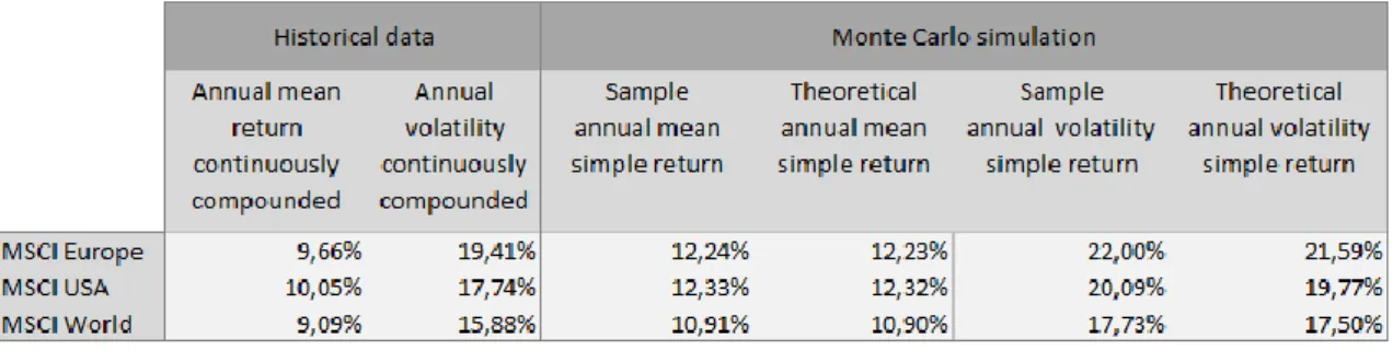
Table 1 depicts the results for the historical annual mean and volatility as well as the simulated annual mean and volatility and their respective theoretical values according to Equation 16. The results of the Monte Carlo simulations are quite close to the theoretical values, indicating that the Monte Carlo simulations provide an adequate degree of accuracy21.

19

Assuming n observation dates and 250 trading days a year, the calculations are as follows

(

), ∑ , , √ ∑ and √

(Benninga, 2008, p. 489).

20

All data is taken from Thompson Reuters Datastream.

21

Beyond that, the accuracy of the simulation results is as well ensured by the insignificantly small standard errors of the Monte Carlo simulations (see section 4.3).

(28)

20

Table 1: Historical annual mean and volatility vs. Monte Carlo simulation values

Then, for each simulation run, the various portfolio insurance strategies are applied. Since all portfolio insurance strategies are rebalanced on a daily basis in order to reduce potential replication errors, the transaction costs effect cannot be neglected. Therefore, for each portfolio shift, 10 basis points round-trip transaction costs are taken into account (Dichtl & Drobetz, 2010; Herold et al., 2007; Hocquard et al., 2012). Additionally, the determination of the initial position does not evolve any transaction costs (Benninga, 1990, p. 22). Furthermore, the synthetic put and the protective put portfolio insurance strategy are implemented with the modified volatility estimator suggested by Boyle and Vorst (1992)22. Besides, in order to maintain a certain protection level, the strike price remains constant during the investment horizon. Following Figlewski et al. (1993, p. 48), the cost of buying the first put for the protective put portfolio insurance strategy is financed by borrowing at the risk-free rate. Thereafter, it is assumed that the expiring put produces a cash inflow equal to the amount by which it was in the money, if any. Then, the next put is either financed by the cash inflow of the expiring put or the reminants are borrowed at the risk-free rate. Any cash left over is invested in the risk-free asset. In order to avoid a high portfolio turnover which is triggered by trendless markets, portfolio shifts are only executed when the market moves by more than 2% (Dichtl & Drobetz, 2010; Do & Faff, 2004). Finally, the corresponding portfolio prospect values of all 100.000 simulation runs are ranked from worst to best, for computing the CPT values of each strategy.

22

Since the assumptions are based on a Geometric Brownian motion that generates log normally distributed stock prices, the Monte Carlo simulations use the sample volatility of the generated stock prices. Usually, traders assume that the lognormal distribution understates the probability of extreme market movements, using the implied volatility instead. For the discussions on implied volatilities, please refer to Hull (2008, pp. 375 - 389). However, Dichtl and Drobetz (2010) find that volatility misestimation does not have a large impact on the CPT value of the synthetic put portfolio insurance strategy.

(29)

21

However, when analyzing the risk of portfolio insurance strategies which are skewed towards positive returns, the standard deviation is not an appropriate risk measure since it assumes symmetry and penalizes upside deviations from the mean as much as downside deviations. In contrast, investors tend to perceive only negative deviations as risk whereas positive deviations are regarded as chances. Lower partial moments (LPM) capture this notion of risk and are defined as (Poddig et al., 2000, p. 136)

Equation 17: Lower partial moments

∑

where m denotes the moments, π the threshold return, ri the portfolio return below

the threshold and n´ the number of observations below the desired threshold. Basically, the moments can be set at any value, but its choice has a strong economic meaning. LPM0 measures the shortfall probability but contains no information on the amount of

loss in case of missing the threshold return. Therefore, LPM1 captures the mean

deviations below the threshold return (expected shortfall), LPM2 indicates the squared

deviations below the threshold return (shortfall variance)23 and √LPM2 indicates the

shortfall deviation. Since a CPT investor evaluates gains and losses in respect to the reference point of his initial wealth, the threshold rate is fixed at 0%, meaning that each negative return will enter the LPM calculations.

Consequently, the sharpe ratio is inadequately as well since it depends on the standard deviation and therefore suffers from the same shortcomings. Instead, the LPMs of the first and second order can be applied for evaluating the risk-adjusted performance of the portfolio insurance strategy. Hence, the return to shortfall (RTS) as a risk-reward ratio is calculated as (Dichtl, 2001, p. 321)

23

In the case of π = μ, the LPM2 is equivalent to the semi variance suggested by Markowitz

(1959) (Poddig et al., 2000, p. 136). However, the LPM measures allow to choose an arbitrary value for the threshold return which is more convenient with behavioral finance since investors separate between gains and losses in respect to the reference point of zero.

(30)

22

Equation 18: Return to shortfall

̅

√

where ̅ denotes the average portfolio return. Consequently, the RTS1 measures the

excess return over the expected shortfall whereas the RTS2 indicates the excess return

over the shortfall deviation.

Moreover, the omega ratio, suggested by Keating and Shadwick (2002) incorporates all higher moments of the return distribution, also skewness and kurtosis. Since risk-averse investors usually prefer investment strategies that are positively skewed (positive skewness) and dislike the probability of less likely but extreme events (high kurtosis), the impact of these higher moments should not be neglected. Consequently, the omega ratio takes the whole return distribution into account and incorporates the impact of gains as well as the effects of losses, relative to the investor´s threshold return π. The omega ratio can be calculated as (Kaplan & Knowles, 2004)

Equation 19: Omega ratio

̅

Although the unbroken popularity of portfolio insurance strategies might not be explained by their risk-reward potential since taking over systematic risk is rewarded with an equity premium, the simulation analysis also accounts for the risk and return measures presented in this section. However, since the optimality of a portfolio insurance strategy depends on the investor´s utility function (Benninga & Blume, 1985), the main focus is on CPT values.

(31)

23

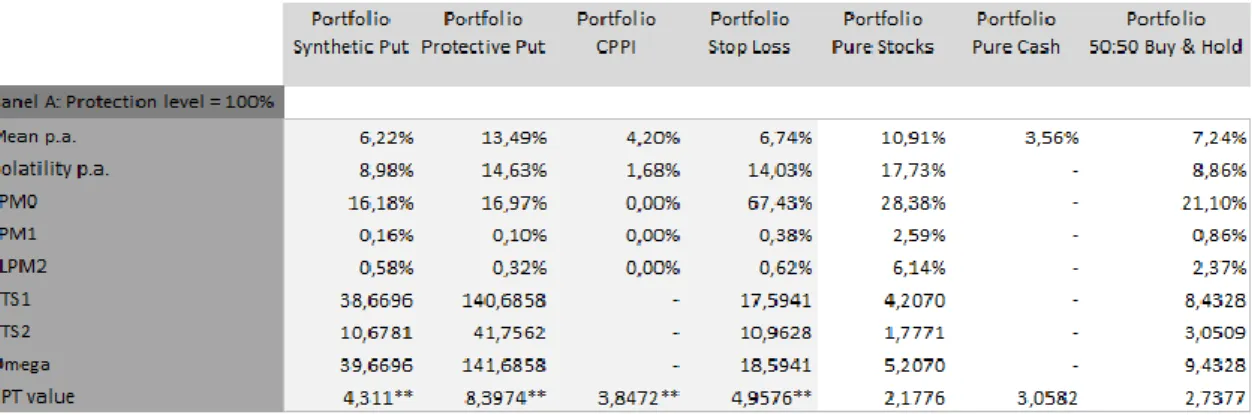
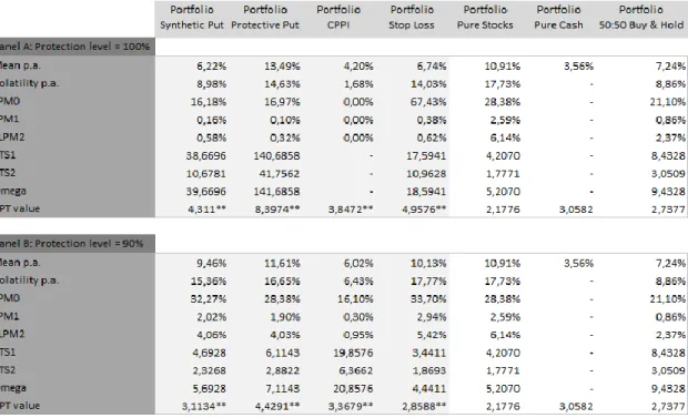
4.2 Base case simulation results

This section presents the base case simulation results. In the base case scenario, all portfolio insurance strategies are implemented with a protection level of 100% since CPT investors consider losses more than twice as important as gains. Furthermore, the CPPI strategy is employed with a multiplier of 2.5 (Dierkes et al., 2010) which means that the risky asset can lose at most 40% without violating the floor. In all investment markets, the annual risk-free rate is fixed at 3.5%24 and the risk-free asset is compounded on a daily basis.

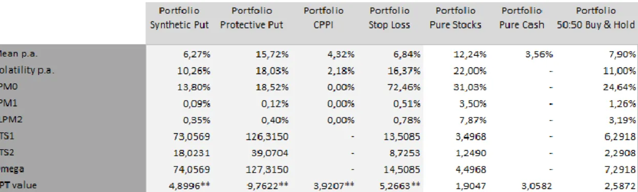
Table 2: Base case Monte Carlo simulation results MSCI Europe

As expected, the stock market investment exhibits the highest annual mean return (apart from the protective put strategy) due to the risk premium effect (12.24%). Although the portfolio insurance strategies provide a reduced return potential, their annual standard deviation is significantly lower in regards to that of the stock market investment. However, since the standard deviation is not an appropriate risk measure, the LPMs provide more liable insight into the risk involved. The LPM0 indicates that the probability

of negative returns is relatively high for the benchmark portfolios (31.03% for the stock investment and 24.64% for the buy and hold investment, respectively), but significantly higher for the stop loss strategy (72.46%). But this mitigates when the LPM1 is taken into

consideration, since the expected shortfall is relatively small (0.51%). A possible explanation for this finding is that the stop loss strategy fails to compensate a sudden

24

Initially, it was intended to calculate the risk-free rate from historical data. However, the corresponding risk-free rate depends as well on the respective market capitalization per country of the MSCI indices. Unfortunately, this information was not available.

(32)

24

loss in stock prices at an early stage of the investment horizon, ending up more often slightly below the pre-specified floor as time elapses. Nevertheless, all portfolio insurance strategies dominate the benchmark strategies in regard to their LPM1 and

√LPM2, indicating significantly lower downside risk. Moreover, the CPPI strategy even

shows no downside risk at all but also yields the lowest annual mean return apart from the cash investment. Hence, the portfolio insurance strategies significantly dominate the benchmark strategies regarding their risk-adjusted returns whereas the RTS1, RTS2 and

omega ratio show the same rankings: the protective put provides the highest risk-reward ratios, followed by the synthetic put, the stop loss strategy and the benchmark strategies25.

When the analysis is based on CPT values, all portfolio insurance strategies dominate the respective benchmark strategies as well. While the stock market investment provides the highest annual mean return, it is the least attractive strategy regarding its CPT value (1.9047). This finding can be explained by both, loss aversion and the probability weighting scheme. Since the passive stock market strategy contains the highest downside risk (LPM1 3.50% and √LPM2 7.87%), the negative CPT values

during one year investment horizon cannot be offset by the positive risk-premium effect. Also, extreme adverse states receive higher probability weights which further contribute to the relatively poor performance of the stock investment regarding its CPT value. More interestingly, the ranking of the CPT values is different from that of the risk-reward ratios. Although the protective put strategy is still the preferable investment strategy, the stop loss strategy is now the second attractive one, followed by the synthetic put strategy, the CPPI strategy and the benchmark strategies. Hence, the CPPI investment strategy seems to be the least attractive portfolio insurance strategy for a CPT investor, despite of not having any downside risk at all. In fact, with an annual mean return of 4.32%, the CPPI strategy exhibits only a slightly better annual mean return than the cash investment (3.56%). However, the different ranking of the risk-reward ratios and the CPT values can once more be explained by the probability weighting scheme: The risk-reward measures only capture the probability of positive and negative outcomes whereas the CPT probability weighting function puts extra weights on the tails of the return distribution, thereby overestimating low probability events. Regarding the poor CPT value of the passive stock market investment (1.9047) compared to that of the buy and hold strategy

25

Since the CPPI portfolio insurance strategy and the cash investment exhibit no downside risk, the risk-reward ratios are not defined.

(33)

25

(2.5872), it seems that several extremely adverse states occurred. Among the benchmark strategies, the money market investment yields the highest CPT value (3.0582) since it earns an annual return without any loss potential. However, although the cash investment seems to be an attractive investment strategy for a CPT investor, it is dominated by all four portfolio insurance strategies regarding its CPT value. A paired t-test26 reveals that the CPT values of the portfolio insurance strategies significantly differ from the CPT value of the cash investment (which is the benchmark strategy yielding the highest CPT value). All differences are statistically significant at the 1% level. Consequently, it seems that portfolio insurance strategies provide an attractive investment strategy for an investor with CPT preferences, whereas the protective put strategy seems to be the most attractive one, followed by the stop loss strategy, the synthetic put strategy and the CPPI strategy.

Table 3: Base case Monte Carlo simulation results MSCI USA

Basically, the Monte Carlo simulation results of the MSCI USA index lead to the same conclusions. Again, the stock market investment yields the highest annual mean return (with the exception of the protective put strategy), whereas the portfolio insurance strategies provide a lower return potential due to the risk premium effect. Also, the LPM0

indicates a high probability of negative returns for the benchmark investments (28.59% for the passive stock investment and 21.97% for the buy and hold strategy) and the stop loss strategy (69.55%), presumably due to the same reasons as explained before since

26

Although there exist more powerful hypothesis tests which take the whole distribution into account (Linton et al., 2005), a paired t-test is frequently used to test the significance in differences of portfolio insurance strategies (Annaert et al., 2009; Dichtl & Drobetz, 2010).

(34)

26

the expected shortfall of the stop loss strategy is negligibly small (LPM1 0.44%). Besides,

the benchmark strategies exhibit significantly higher shortfall deviations than the portfolio insurance strategies (√LPM2 2.90% for the stock strategy and 1.00% for the buy and hold

strategy, respectively) which are once more reflected in the risk-reward ratios. Surprisingly, the ranking of the risk-reward ratios is equal to that of the CPT values (apart from the CPPI strategy and the cash investment since their risk-reward ratios are not defined). Hence it seems that less extreme negative events occurred whose impacts on CPT values are not that severe. This assumption is even more likely since the difference between the CPT value of the stock investment (2.5635) and the buy and hold investment (2.9330) is not that pronounced as in the MSCI Europe simulation (Table 1). However, the portfolio insurance strategies again dominate the corresponding benchmark strategies regarding their CPT values. As a paired t-test reveals, the CPT values of the portfolio insurance strategies significantly differ from that of the cash investment (which is again the benchmark with the highest CPT value). All differences are statistically significant at the 1% level.

Table 4: Base Case Monte Carlo simulation results MSCI World

Once more, the Monte Carlo simulation of the MSCI World index leads to the same results. Apart from the protective put strategy, the stock market investment and the buy and hold investment dominate the portfolio insurance strategies in regard to their annual mean returns (10.91% and 7.24%, respectively) but compare unfavorably regarding their risk measures. Besides, the risk-reward ratios and CPT values rank the investment strategies differently, thereby indicating the occurrence of extremely adverse events. However, since the difference between the CPT value of the passive stock investment

(35)

27

(2.1776) and the buy and hold investment (2.7377) is not that large in magnitude, it seems that only few extremely adverse states occurred. Again, all portfolio insurance strategies significantly dominate the respective benchmark portfolios regarding their CPT values at the 1% level. For an investor with CPT preferences, the protective put strategy is once more the most attractive portfolio insurance strategy, followed by the CPPI strategy, the synthetic put strategy and the stop loss strategy.

When comparing the results of all three Monte Carlo base case simulations, the following patterns are observable: Regarding the fact that the Monte Carlo simulations of the MSCI Europe and MSCI USA indices yield almost the same stock markets returns (12.24% and 12.33%) but different volatilities (22% and 20.09%), it seems that the higher the volatility, the better the CPT values of the portfolio insurance strategies (Table 2 and Table 3, respectively). This observation can be explained by the high degree of loss aversion which is also consistent with the findings of Hwang and Satchell (2010, p. 2437) that investors are more risk averse than usually assumed. Furthermore, in the absence of extremely adverse states, it seems that the ranking of the risk-reward ratios is equal to that of the CPT values but it differs in the case of extreme outcomes. One possible explanation of this finding is the probability weighting scheme: The risk-reward ratios only capture the probability of positive and negative outcomes whereas the CPT probability weighting function puts extra weights on the tails of the return distribution, thereby overestimating low probability events. However, the main result is not affected by differences in volatilities and rankings of the investment strategies. All three stock market simulations provide qualitatively similar results as the portfolio insurance strategies dominate – without any exception - the benchmark strategies regarding their CPT values. This is also consistent with the findings of Dichtl and Drobetz (2010). Nevertheless, in order to gain more detailed insight, an extensive sensitivity analysis is conducted.

4.3 Sensitivity analysis

When changing the input parameters for conducting the sensitivity analysis, the same 100.000 price series of each particular MSCI index is used. Although this might lead to some bias because the same sampling error enters into the results, using the same price series allows for a better comparison of the behavior of the investment strategies (Figlewski et al., 1993, p. 50). Nevertheless, since the accuracy of the

(36)

28

simulation result highly depends on the number of trials, the standard errors of each Monte Carlo simulation are computed as (Hull, 2008, p. 414)

Equation 20: Standard error of Monte Carlo simulation

√

whereas M denotes the number of trials. Given a sampling error of 0.06% for the Monte Carlo simulations MSCI Europe index, 0.05% for the MSCI USA index and 0.04% for the MSCI World index, respectively, the simulation results of 100.000 simulation runs provide an adequate degree of accuracy27, indicating qualitatively good simulation results.

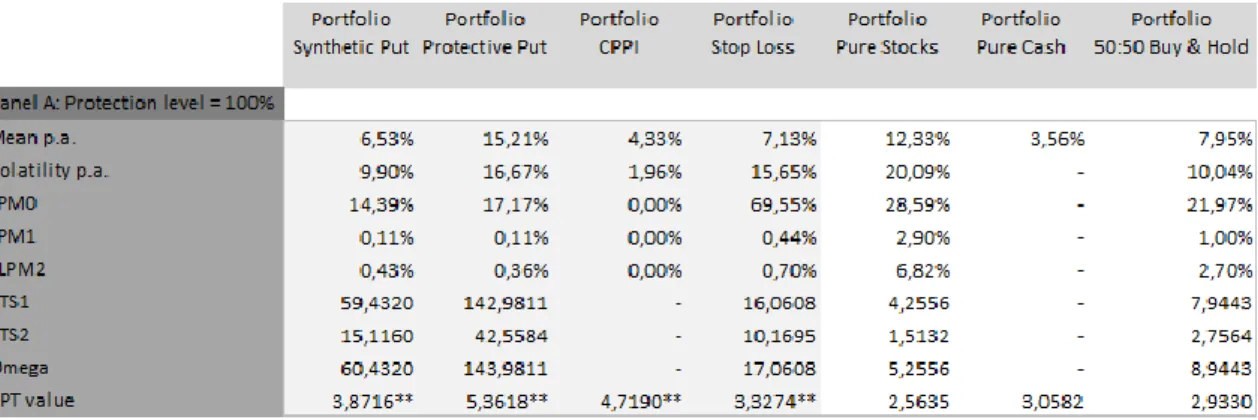
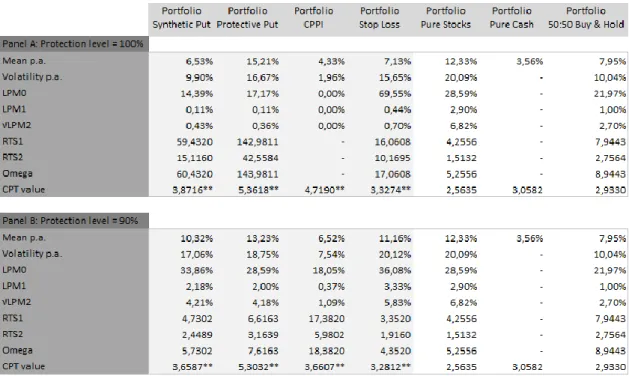
4.3.1 Varying the protection level

Since CPT investors are very sensitive to the possibility of losses, the impact of changing the protection level cannot be neglected. However, the higher the protection level, the lower the respective return potential. It is unclear if a higher return potential can compensate for the reduced protection level regarding CPT values. Therefore, the Monte Carlo simulations are repeated with a 90% protection level.

27

The accuracy of the simulation results was already confirmed by the results shown in Table 1 since the theoretical values for the annual mean return and volatility are very close to the simulated ones.

(37)

29

Table 5: Monte Carlo simulation results MSCI Europe: Varying the protection level

As expected, the annual mean returns as well as the downside risk measures increase when the floor is reduced. As the LPM0 indicates, nearly all portfolio insurance

strategies exhibit significantly higher shortfall probabilities: the synthetic put strategy (13.80% vs. 37.48%), the protective put strategy (18.52% vs. 31.03%) and the CPPI strategy (0% vs. 21.58%) which does not even relax by taking the LMP1 into account.

Moreover, the shortfall deviations of the synthetic put strategy (√LPM2 4.55%) and the

protective put strategy (√LPM2 4.49%) are significantly higher than that of the buy and

hold strategy (√LPM2 3.19%), whereas the stop loss portfolio strategy even exhibits a

shortfall deviation comparable to that of the passive stock investment (√LPM2 6.33% vs.

7.87%). The CPPI strategy provides the only exception regarding its downside risk measures, still containing the lowest shortfall deviation (√LPM2 1.31%). Consequently,

the risk-reward ratios reflect the poor performance of the portfolio insurance strategies at a lower protection level. This is particularly pronounced for the synthetic put strategy and stop loss strategy since they are dominated by the buy and hold strategy whereas the stop loss strategy is even partly dominated by the stock investment. However, according to risk-reward ratios no clear dominance can be found: some portfolio insurance strategies dominate the benchmark strategies regarding their risk and return measures but some are dominated.

(38)

30

Again, a paired t-test reveals that the differences in CPT values between the money market investment (being the best performing benchmark strategy in terms of its CPT value) and the portfolio insurance strategies are highly significant at the 1% level. In contrast to the findings of Dichtl and Drobetz (2010) that all portfolio insurance strategies implemented with a 90% protection level are dominated by the cash investment regarding their CPT values, only the stop loss portfolio insurance strategy exhibits a significantly lower CPT value than the money market investment (2.9413 vs. 3.0582). As the LPM0 indicates, the probability of earning a loss is significantly lower at the 90%

protection level (40.46% vs. 72.46%) but the corresponding loss is large in magnitude (√LPM2 6.33% vs. 0.78%). Although the stop loss strategy yields a relatively high annual

mean return (10.82%), CPT investors care more than twice as much about potential losses than about potential gains. Therefore they prefer the cash investment without any loss potential over the stop loss portfolio insurance strategy implemented at a lower protection level. For the protective put strategy, on the other hand, the probability of earning a loss is significantly higher when implemented with a 90% protection level (LPM0 31.03% vs. 18.52%), but it seems the high shortfall deviation (√LPM2 4.99%)

results from some extremely adverse events whose negative effects could be offset by the positive prospect values of many good states, as the high annual mean return indicates (13.48%). Additionally, the different ranking of the risk-reward ratios and the CPT values indicate probability distortions, thereby supporting this assumption. However, apart from the stop loss portfolio insurance strategy, the portfolio insurance strategies again significantly dominate the corresponding benchmark strategies regarding their CPT values.