Yanzhen Liu, Xiao Bai, Haichuan Yang, Zhou Jun, and Zhihong Zhang
Springer-Verlag, Computer Science Editorial, Tiergartenstr. 17, 69121 Heidelberg, Germany
{alfred.hofmann,ursula.barth,ingrid.haas,frank.holzwarth, anna.kramer,leonie.kunz,christine.reiss,nicole.sator,
erika.siebert-cole,peter.strasser,lncs}@springer.com http://www.springer.com/lncs
Abstract. Hashing is a popular solution to Approximate Nearest Neigh-bor (ANN) problems. Many hashing schemes aim at preserving the Eu-clidean distance of the original data. However, it is the geodesic distance rather than the Euclidean distance that more accurately characterizes the semantic similarity of data, especially in a high dimensional space. Consequently, manifold based hashing methods have achieved higher ac-curacy than conventional hashing schemes. To compute the geodesic dis-tance, one should construct a nearest neighbor graph and invoke the shortest path algorithm, which is too expensive for a retrieval task. In this paper, we present a hashing scheme that preserves the geodesic dis-tance and use a feasible out-of-sample method to generate the binary codes efficiently. The experiments show that our method outperforms several alternative hashing methods.
Keywords: Hashing, Manifold, Isomap, Out-of-sample extension
1
Introduction
Nearest Neighbor (NN) search is a basic and important step in image retrieval. For a large scale dataset of sizen, the complexity of NN search isO(n), which is still too high for big data processing. To solve this problem, sublinear ap-proximate nearest neighbor methods have been proposed. Hashing methods are among such well-performed methods.
The basic idea of hashing is to use binary code to represent high-dimensional data, with similar data pair having smaller Hamming distance of binary codes. In other words, we should construct a mapping from high-dimension Euclidean space to Hamming space and preserve the original Euclidean distance of data in the Hamming space. We can see that hashing accelerates NN search on two aspects: one is that binary XOR operation to calculate the Hamming distance is much faster than calculating the Euclidean distance; the other is that binary code can be used as address to index the original data.
A simple and basic hash method is Locality-Sensitive Hashing(LSH) [2]. LSH is based on generating random hyperplane in Euclidean space. A hyperplane
generates a bit of code. Data points on one side of the hyperplane are coded 0 at this bit, while at the other side are coded 1. Critically, points on the hyperplane can be coded either 0 or 1, but the probability is very low. LSH successfully reduces the hashing process to sublinear query time with acceptable accuracy. However, because of its randomness, reaching higher accuracy needs longer code, and there is redundancy to some degree.
To get more compact binary code, some researchers started to analyze the inner structure of dataset. These efforts led to data-dependent hashing methods while LSH is data-independent method. Among the data-dependent methods, some are linear such as Iterative Quantization (ITQ) [7] and some are non-linear such as Spectral Hashing (SH) [14], and Anchor Graph Hashing (AGH) [9]. By learning the inner structure of dataset, the hash codes gain higher accuracy with shorter code length.
Although all the above hashing methods are concentrating on preserving Euclidean distance, however, the most similar data pair may not be the nearest neighbor in Euclidean space, but the nearest neighbor on the same manifold. Thus if we want to improve the precision of hashing method, we must take manifold structure into consideration as well. For linear manifold, linear methods such as PCAH, PCA-ITQ is applicable. But for non-linear manifold such as Swiss Roll, further exploration is needed to catch the manifold structure in hashing.
Graph methods play an important role in image analysis [15–17]. Many non-linear manifold learning methods are motivated by graph approaches that create low-dimension embedding of data with manifold distribution in Euclidean space, such as Laplace Eigenmap (LE) [3], Locally Linear Embedding (LLE) [11], and Isometric Mapping (ISOMAP) [13]. Some manifold based hashing methods uti-lize these ideas and extend them to embedding in Hamming space, such as Inducitve Manifold Hashing (IMH) [12] and Locally Linear Hashing (LLH) [6]. IMH-tSNE extracts manifold structure with tSNE [1] and gives an out-of-sample extension scheme by locally linear property of manifold. LLH learns the locally-linear structure of manifold and preserves it in hash code.
In this paper, we utilize a widely used non-linear dimensionality reduction method Isometric Mapping (ISOMAP) to catch the geodesic distance structure of manifold and preserve it in hash code. We name the method Isometric Map-ping Hashing (IsoMH). The experiments show that our IsoMH have comparable precision with the state-of-the-art methods.
2
Isometric Mapping Hashing
Given a set of data points X = [x1,x2, ...,xn] T
xk∈Rd, X∈Rn×d, we want to get a mapping from X to a binary hash code set B ∈ {−1,1}n×c that the hamming distance inB best approximates the data similarity in X.
Here, we explore the geodesic distance on manifold rather than the Euclidean distance as the quantitative measurement of data similarity. So in the process of mapping, we choose to preserve geodesic distance between data points inX and
then use a non-linear dimension reduction method ISOMAP (Section 2.1). Af-ter dimension reduction with ISOMAP, we got the low-dimensional embedding Y ∈ Rn×c, and we quantize Y into a binary hash codeB. Direct quantization with sign functionB =sign(Y) may lead to great quantization loss. Therefore, we employ the iteration quantization method ITQ [7] to calculateB, which sig-nificantly reduces the quantization loss (Section 2.2). Finally we use an efficient out-of-sample extension method rather than doing ISOMAP again for a single data query (Section 3). The experiments to evaluate our method is introduced in Section 4.
Here is a list of mathematical symbols appearing in the following sections: b: number of bits of the final hash code.
ξ: eigenvector of the kernel matrix.
V: eigenvector matrix,V = (ξ1, ξ2, ..., ξb)T.
λ: eigenvalue of the kernel matrix Λ: diagonal matrix of eigenvalues. y: embedding vector.
Y: data matrix,Y = (y1,y2, ...,yb)
T . B: binary code matrix.
2.1 Dimensionality Reduction with ISOMAP
Isomap is a non-linear dimensionality reduction method which aims at preserving the geodesic distance of the manifold structure. Real geodesic distance is difficult to compute, so Isomap takes shortest path distance to approximate the geodesic distance in large dataset.
With the datasetX, we can construct a neighborhood graphG, whose edges connect only neighboring nodes with the Euclidean distance of neighboring nodes as the weights. To properly define the neighborhood, we set a threshold. Only node pairs whose Euclidean distances are below the threshold are considered as neighboring nodes. Alternately, we can choose a number k, only node pairs being k-nearest-neighbor to each other are regarded as neighboring. With this neighborhood graphG, we compute the shortest path distance between all node pairs inGto approximate the geodesic distance of those node pairs. We denote the approximate geodesic distance matrix asD.
When using the Euclidean distance to reduce dimensionality, we come up with Multidimensional Scaling (MDS) [5]. MDS is a linear dimension reduction method aiming at preserving the pairwise distance. According to [5], we can get the low-dimensional embedding by decomposing the kernel matrix
K=−1
2HDH (1)
where H =E−1
tee
T. (What ise?) We pick eigenvectors ξ
k(16k6b) of the topbeigenvaluesλk(16k6b) ofK. Then the low-dimensional embedding can be calculated as
2.2 Quantize low-dimension embedding with ITQ
After getting the low-dimension embedding Y, we are able to quantize it into binary code. In order to get the binary code, we need to quantize each dimension in the low-dimensional embedding into 0 and 1 according to the formula
B =sign(Y) (3)
Direct quantization may cause great loss as explained in [7]. So we try to calculate an optimized rotation matrix to minimize the quantization lossQ.
Q=kB−Y RkF (4)
Tackling this optimization problem, an iterative method was proposed to solveB andRone after the other [7]. When solvingB, we fixRand calculateB with sign function B =sign(Y R). When solvingR, we fixB and the problem becomes the classic Orthogonal Procrustes Problem. It can be solved by com-puting the Singular Value Decomposition (SVD) of BTV as SΩSˆ, and we get R = ˆSST. Finally, we get a local minimum of the quantization lossQ and its corresponding optimal rotation matrixR. Then binary hash code of training set can be represented asB=sign(Y R).
The whole process of training is described in pseudo-code in Algorithm 1.
Algorithm 1: Training phase of Isometric Mapping Hashing
Data: training dataX, code lengthb
Result: shortest path matrixD, eigenvector matrixV, eigenvalue matrixΛ,
Euclidean embeddingE, rotation matrixR, hash codeB
Compute Euclidean distances of all data points; Sort Euclidean distances to identify neighborhoods;
Construct adjacency matrixAof neighborhood graph G;
Calculate shortest path distanceDof graph G;
Execute MDS on D and getV,ΛandY;
Execute ITQ on E to get the best quantization codeB, with rotation matrixR;
3
Out-of-Sample Extension
By applying the above described method on the training set, we can get the binary codes of the whole set.If we get a single testing data, we must calculate all other training data together with this single testing data. With the shortest path distance and matrix decomposition, the Isomap takesO(n3) to execute, which is difficult to meet the need of online query. To solve this problem, we adopt an out-of-sample extension method [4] to calculate the approximate Isomap embedding. Given a queryq, we first need to calculate its approximate geodesic distance to all other training set points, and that is, to calculate its shortest path distance
to all others. In fact, there is no need to run Dijkstra one more time. If the neighborhood ofqisxl1,xl2, ...,xlk(16li6n), then the shortest path distance of qto all other point inX can be calculated by the shortest path distance of its neighbors. Denoting byD(xi,xj), the shortest path distance fromxi toxj, it is obvious that
D(x,q) = min
i {kq−xlik+D(xli,x)} (5) To calculate a pair of shortest path distance, we just need to compare k-1 times and add k times.
With the newly calculatedD(x,q), we can calculate the embeddingyof an out-of-samplexaccording to the expression
yk(q) = 1 2 1 √ λk n X i=1 vki Ex0 h D2x0,xi i −D2(xi,q) (6)
given in [4]. And it can be represented in matrix as y= 1 2Λ 1 2V η (7) whereη=Ex0 h D2x0,·i−D2(q,·) is a column vector.
The pseudo-code of out-of-sample extension is written as follow.
Algorithm 2: Out-of-sample Extension
Data: training dataX, code lengthb, shortest path matrixD, eigenvector
matrixV, eigenvalue matrixΛ, Euclidean embeddingY,rotation matrix
R, hash codeB, out-of-sampleq
Result: hash code of out-of-sample databq
Compute Euclidean distances ofxq to all training data;
Decide thekneighborhood point set ofq:xl1,xl1, ...,xlk;
Calculate shortest path distancedq fromqto all other training data according
to equation(5);
Calculate Euclidean embeddingyq of out-of-sample point according to
equation(6);
bq=RTsign(yq);
4
Experiments
We ran experiments to test our IsoMH method on two frequently-used image datasets: MNISTandCIFAR-10[8].
MNIST. The MNIST dataset has 70000 28*28 small grayscale images of handwritten digits from ’0’ to ’9’. Each small image is represented by a 784-dimensional vector and a single digit label. We used 2000 random images as the training set, and 500 random images as the query set.
Fig. 1.Images in the left column are query images selected from 10 classes, and the rest images are the retrieval results using IsoMH. Images in green boxes represent the correct results.
CIFAR-10. There are 60000 32*32 small color images in CIFAR10. These small images are from 10 classes: airplane, automobile, bird, cat, deer, dog, frog, horse, ship, and truck. Each class has 6000 images. Every image inCIFAR10is represented by a 320-dimensional GIST feature [10] vector and a label from ‘1’ to ‘10’. Fig. 1 shows sample results onCIFAR-10. We selected 10 images from different classes as the query and search the top 9 nearest neighbors in hamming distance of hash codes.
Besides IsoMH, we also tested other 5 unsupervised methods: LSH [2], PCA-ITQ [7], AGH [9], IMH-LE, and IMH-tSNE [1]. LSH and PCA-PCA-ITQ are linear while AGH, IMH-LE and IMH-tSNE are nonlinear. Specifically, two IMH meth-ods are also manifold based. We used codes released by the original authors during the experiments.
Manifold based methods aim at getting semantically similar results. Though unsupervised, we used class labels as the ground truth, and evaluated the perfor-mance of those methods by Precision-Recall (P-R) curves and time consumption of training and query. We calculated the precision and recall by:
precision=Number of retrieved true neighbor pairs
Number of retrieved neighbor pairs (8) recall= Number of retrieved true neighbor pairs
Total number of true neighbor pairs (9) All our experiments were run on a 64-bit PC with 3.50 GHz Intel i7-4770K CPU and 16.0GB RAM.
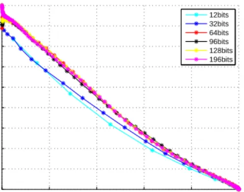
4.1 Parameters Analysis 0 0.2 0.4 0.6 0.8 1 0.1 0.2 0.3 0.4 0.5 0.6 0.7 0.8 0.9 1 MNIST Recall Precision 12bits 32bits 64bits 96bits 128bits 196bits
Fig. 2. The Precision-Recall curve of IsoMH with different hash code length on the MNIST dataset.
We set the hash code length to 12bits, 32bis, 64bits, 96bits and 128bits and performed the experiments, respectively. The results are shown in Fig 2. The curves show that when the number of bits is small, results will be better with the increasing of code length, and if the code length is large enough, adding hash bits cannot bring much advance in retrieval precision.
For the construction of nearest neighbor graph, different methods and pa-rameters have almost the same results with shortest path distance algorithm, because the training set is large. In our experiments, we setk= 7.
4.2 Comparison to Other Methods
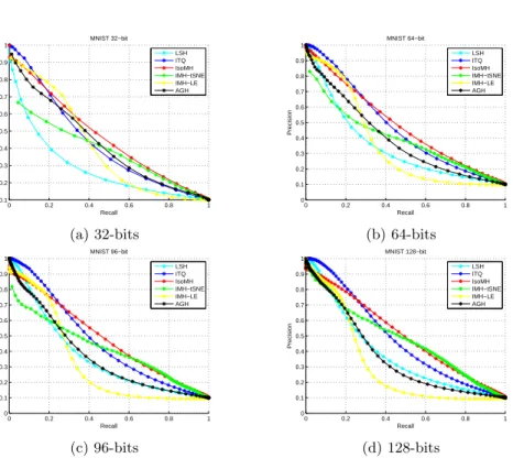
Fig. 3 shows the P-R curves of the above-mentioned methods on MNIST. Our IsoMH performs better than all other methods. Linear method PCA-ITQ and manifold method IMH-tSNE are two most competitive methods. As the figure showing, IMH-tSNE performs better with longer code. For the training time
0 0.2 0.4 0.6 0.8 1 0.1 0.2 0.3 0.4 0.5 0.6 0.7 0.8 0.9 1 MNIST 32−bit Recall Precision LSH ITQ IsoMH IMH−tSNE IMH−LE AGH (a) 32-bits 0 0.2 0.4 0.6 0.8 1 0 0.1 0.2 0.3 0.4 0.5 0.6 0.7 0.8 0.9 1 MNIST 64−bit Recall Precision LSH ITQ IsoMH IMH−tSNE IMH−LE AGH (b) 64-bits 0 0.2 0.4 0.6 0.8 1 0 0.1 0.2 0.3 0.4 0.5 0.6 0.7 0.8 0.9 1 MNIST 96−bit Recall Precision LSH ITQ IsoMH IMH−tSNE IMH−LE AGH (c) 96-bits 0 0.2 0.4 0.6 0.8 1 0 0.1 0.2 0.3 0.4 0.5 0.6 0.7 0.8 0.9 1 MNIST 128−bit Recall Precision LSH ITQ IsoMH IMH−tSNE IMH−LE AGH (d) 128-bits
Fig. 3.Precision-Recall curves of different methods with experiments on the MNIST dataset.
Methods 32 bits 64 bits 96 bits 128 bits
Training Indexing Training Indexing Training Indexing Training Indexing
IsoMH 1853.44 189.03 1901.18 193.63 1954.06 211.14 2048.67 232.61
PCA-ITQ 10.61 0.18 18.27 0.35 29.78 0.50 42.52 0.69
IMH-tSNE 35.01 1.09 69.02 1.13 85.92 1.22 95.07 1.18
IMH-LE 96.38 2.20 90.61 2.20 87.13 2.52 87.99 2.28
AGH 84.02 10.92 87.42 13.35 84.97 13.20 85.47 13.09
consumption, as shown in Table 1, our method is not very competitive because the time complexity of shortest path algorithm is O(n3). In P-R curve, our IsoMH performs better in middle and lower precision region while be weaker in higher precision region.
Fig. 4 shows the P-R curves of results on CIFAR-10. CIFAR-10 has more complex images than MNIST so these P-R curves are lower than MNIST’s. And our IsoMH is still better than all the curves.
0 0.2 0.4 0.6 0.8 1 0 0.1 0.2 0.3 0.4 0.5 0.6 0.7 0.8 0.9 1 CIFAR−10 32−bit Recall Precision LSH ITQ IsoMH IMH−tSNE IMH−LE AGH (a) 32-bits 0 0.2 0.4 0.6 0.8 1 0 0.1 0.2 0.3 0.4 0.5 0.6 0.7 0.8 0.9 1 CIFAR−10 64−bit Recall Precision LSH ITQ IsoMH IMH−tSNE IMH−LE AGH (b) 64-bits 0 0.2 0.4 0.6 0.8 1 0 0.1 0.2 0.3 0.4 0.5 0.6 0.7 0.8 0.9 1 CIFAR−10 96−bit Recall Precision LSH ITQ IsoMH IMH−tSNE IMH−LE AGH (c) 96-bits 0 0.2 0.4 0.6 0.8 1 0 0.1 0.2 0.3 0.4 0.5 0.6 0.7 0.8 0.9 1 CIFAR−10 128−bit Recall Precision LSH ITQ IsoMH IMH−tSNE IMH−LE AGH (d) 128-bits
Fig. 4.Precision-Recall curves of different methods with experiments on the CIFAR-10 dataset.
5
Conclusion
Manifold based hashing methods have advantages on retrieving semantically similar neighbors. In this paper, we preserve geodesic distance of manifold with binary code and utilize ISOMAP to implement our mapping. IsoMH outper-forms many state-of-the-arts methods in precision but consume more time in computing the shortest distance of neighborhood graph. In the future work, we will concentrate on improving the time efficiency of IsoMH.
Acknowledgement
This research is supported by National Natural Science Foundation of China (NSFC) projects No. 61370123 and No.61402389.
References
1. Visualizing data using t-SNE], author = Van der Maaten, Laurens and Hinton, Geoffrey, journal = Journal of Machine Learning Research, year = 2008, number = 2579-2605, pages = 85, volume = 9
2. Andoni, A., Indyk, P.: Near-optimal hashing algorithms for approximate nearest neighbor in high dimensions. In: Foundations of Computer Science, 2006. FOCS’06. 47th Annual IEEE Symposium on. pp. 459–468. IEEE (2006)
3. Belkin, M., Niyogi, P.: Laplacian eigenmaps and spectral techniques for embedding and clustering. In: NIPS. vol. 14, pp. 585–591 (2001)
4. Bengio, Y., Paiement, J.f., Vincent, P., Delalleau, O., Roux, N.L., Ouimet, M.: Out-of-sample extensions for LLE, Isomap, MDS, eigenmaps, and spectral clustering. In: Advances in Neural Information Processing Systems. pp. 177–184 (2004) 5. Cox, T.F., Cox, M.A.: Multidimensional Scaling. CRC Press (2010)
6. Go, I., Zhenguo, L., Xiao-Ming, W., Shih-Fu, C.: Locally linear hashing for extract-ing non-linear manifolds. In: Computer Vision and Pattern Recognition (CVPR), 2014 IEEE Conference on (2014)
7. Gong, Y., Lazebnik, S., Gordo, A., Perronnin, F.: Iterative quantization: A pro-crustean approach to learning binary codes for large-scale image retrieval. IEEE Transactions on Pattern Analysis and Machine Intelligence 35(12), 2916–2929 (2013)
8. Krizhevsky, A., Hinton, G.: Learning multiple layers of features from tiny images. Master’s thesis, Department of Computer Science, University of Toronto (2009) 9. Liu, W., Wang, J., Kumar, S., Chang, S.F.: Hashing with graphs. In: Proceedings
of the 28th International Conference on Machine Learning (ICML-11). pp. 1–8 (2011)
10. Oliva, A., Torralba, A.: Modeling the shape of the scene: A holistic representation of the spatial envelope. International journal of computer vision 42(3), 145–175 (2001)
11. Roweis, S.T., Saul, L.K.: Nonlinear dimensionality reduction by locally linear em-bedding. Science 290(5500), 2323–2326 (2000)
12. Shen, F., Shen, C., Shi, Q., Van Den Hengel, A., Tang, Z.: Inductive hashing on manifolds. In: Computer Vision and Pattern Recognition (CVPR), 2013 IEEE Conference on. pp. 1562–1569. IEEE (2013)
13. Tenenbaum, J.B., De Silva, V., Langford, J.C.: A global geometric framework for nonlinear dimensionality reduction. Science 290(5500), 2319–2323 (2000)
14. Weiss, Y., Torralba, A., Fergus, R.: Spectral hashing. In: Advances in neural in-formation processing systems. pp. 1753–1760 (2009)
15. Xiao, B., Hancock, E.R., Wilson, R.C.: Graph characteristics from the heat kernel trace. Pattern Recognition 42(11), 2589–2606 (2009)
16. Xiao, B., Hancock, E.R., Wilson, R.C.: Geometric characterization and clustering of graphs using heat kernel embeddings. Image and Vision Computing 28(6), 1003– 1021 (2010)
17. Zhang, H., Bai, X., Zhou, J., Cheng, J., Zhao, H.: Object detection via structural feature selection and shape model. IEEE transactions on image processing 22(11-12), 4984–4995 (2013)