Inventory Models in Reverse Logistics

Corvinus University Budapest

Faculty of Business Administration

Inventory Models in Reverse Logistics

PhD Dissertation

by

Dobos Imre

November, 2006.

Contents

Preface 3

1. Reverse Logistics: A Framework 4

2. Economic Order Quantity Models in Reverse Logistics 17

2.1. A Reverse Logistics Model with Procurement and Repair 20 2.2. A Model with Procurement and Finite Repair Rate:

The Substitution Policy 33

2.3. A Model with Procurement and Finite Repair Rate:

The Continuous Supplement Policy 46

3. Inventory Models with Waste Disposal 55

3.1. A Repair Model with Three Stocking Point 57

3.2. A Recoverable Item Inventory System 68

3.3. A Production-Recycling Model with Buybacking 83

4. Production Planning in Reverse Logistics 100

5. Summary and Further Research 119

Preface

Environmental conscious material and inventory management will be studied in this dissertation. It is named as reverse, inverse, or waste disposal logistics in the last decade. In the Hungarian literature there are no uniform definitions for this scientific area. This research field is defined in English speaking countries as reverse logistics. A former name of this idea was inverse logistics, but this name is used mainly in Japan.

The dissertation consists of three chapters. In the first chapter I define reverse logistics and its problems.

In the second chapter I present six deterministic reverse logistics inventory models. These inventory models were constructed in the last three decades. A natural extension of EOQ-type inventory models was examined in the last decade. The first reverse logistic inventory model was built in 1967. The second model was published in 1979. In the eighties no paper was published on this research area. The European Union has aided some research projects in the nineties to support European environmental regulation. The publication of new reverse logistic inventory models is in progress nowadays. Main point of the research is now inventory models with shortage. The dissertation contains all available deterministic EOQ-type models without shortage.

The last chapter investigates shortly the influence of reverse logistics on production planning, and on material requirements planning systems. EOQ-type reverse logistics models can be used, as a basis for the dynamic lot size reverse logistic model. The first publication appeared on this field in 2000. The solution of Wagner-Whitin-type reverse logistic model is not easy, because of the complexity of dynamic programming algorithms. EOQ-type reverse logistic models can serve as heuristics to solve such kind of inventory models. This is a potential application of this research field.

1. Reverse Logistics: A Framework

1.1. Introduction

Collection of used products, as paper, bottle, and battery, is a known idea in modern economies. Reuse, remanufacturing and recycling of cars and electronic appliances, and disposal of hazardous waste are very recent research field. The listed activities include a very broad area, and it seems to have different management problems. This chapter summarizes the reverse logistics which offers a theoretical background to solve such kind of business problems.

The reuse is not a new phenomenon in the practice, but a lot of publications are appeared in the international literature in eighties, named reverse logistics. In Hungarian literature there are only a few publications on this research field. The first publication is paper of Rixer (1995). He has called this field as “inverse logistics”. Cselényi et al. (1997) has used the expression “recycling logistics”, and Mike (2002) has given the name “reverse logistics” which is used in English speaking countries. There are some new publications about reverse logistics in Hungarian, as well. (Richter and Dobos (2003)), Dobos (2004)) Reverse logistics includes not only the material flow from supplier to consumer, but also the material flow of used products from consumer to producer and supplier, in order to reduce the burden of environment.

The aim of this chapter is to present the international (mainly Anglo-Saxon) literature on this field. The environmental regulation becomes rigorous in the European Union and in Hungary. There are recently a lot of environmental regulations about wastes along the life cycle of a product in the European Union. (For example, about used cars.)

The European Union plans to solve environmental problems in the near future by the help of legal regulation. These include the use of renewable environmental resources and energy; avoid wastes, and substitution of non-renewable resources.

resources, and to reduce the environmental load, in order to promote sustainable development and economic growth. The law disposes of wastes and activities of its handling. This law does not touch the emissions in the air, and nuclear hazardous wastes. Some of principles are mentioned in this law, as prevention, responsibility of producer, divided responsibility, pollutant pays principle, best available technique, cost efficiency, and so on. The law disposes of responsibility of producers, retailers, consumers, and owners of wastes. Steps of waste management and reuse, and explanation of ideas are included in the law. There are defined collection and transportation of wastes, reuse of wastes and handling. Separate sections present responsibility of handling of communal and hazardous wastes, and organization of waste management. It is to emphasize obligation of publicity and information.

Firms must keep this law, but application of reverse logistic methods can lead to cost savings in long range. Legal registration can not force enterprise to produce an environmental conscious way, but economic earnings can result an environmental friendly production structure of firms.

In this chapter I present shortly the development of reverse logistics, and then I show a conceptual framework, considering the development of this idea in the last decades. After that I look for answer the main questions of reverse logistics: “why-how-what-who”. And last I analyze the participants of reverse logistics, examined the main management problems.

1.2. About development…

There were economic and historic causes of development of logistics, as it is for the reverse logistics. Retailers have recognized the chance of takeback of products in the United States at the end of eighties, as a tool of market growth. Control of takeback was not directed, because there was no uniform and serious regulation of forms of return policies of used products. The result of this development was that consumers have taken back a number of products. The costs of this process have dramatically increased at the producers and at the retailers, which has reduced the profitability and competitiveness of firms. They have recognized that an effective reverse logistics system is an important integral part of corporate strategy of firms. The importance of reverse logistics is out of question, but the application of this concept

reverse logistics concepts differs from each other at firm level. Because of this difficult applicability, I try to define the idea, and I determine the potential research fields of reverse logistics.

1.2.1. Determination of the concept

The reverse logistics was first defined in the eighties. In this time there were published only a few articles in the literature, so the theoretical basis of investigations was unsettled. One of the first publications on this field is the paper of Lambert and Stock (1981). They have defined reverse logistics, as a reverse material flow opposite to supply chain, which is a “bad” process along the material flow of firms. It means that until material flow of traditional supply chain occurs in supplier-producer-wholesaler-retailer-consumer chain, reverse logistics seizes the return material flow of used products, in order to follow this process backward from consumer to supplier.

After the negative definition of Lambert and Stock, Murphy and Poist (1989) have offered a new approach to determine reverse logistics. They have defined reverse logistics, as a material flow of products from consumers to producers in the supply chain. This definition is accepted by Pohlen and Farris (1992), who prefer to apply marketing concepts to reverse logistics. The importance of their paper is that they have named the final consumer, and they have emphasized that the process is reverse in the supply chain. A drawback of this definition is that they have not determined the main activities of reverse logistics, which makes more difficult to limit the framework of reverse logistics.

In the nineties Stock (1992) has given a wide definition, which is a basis for waste management. He stresses the role of logistics, which contains recycling, waste disposal, substitution of hazardous material, reduction of resources, and reuse. This definition of Stock is more accurate than that of earlier. The connection with supply chain activities is missing in this general definition, and the reverse process is not emphasized, as well.

These last approaches are summarized by Kopicky et al. (1993). This definition contains all above-mentioned activities, the reverse movement of materials along the supply chain,

definition of reverse logistics, which helps on effective practical functioning of reverse logistic systems.

Carter and Ellram (1998) have collected a number of definitions of reverse logistics. I will cite one of the definitions. The more general definition is: “Reverse logistics is such an activity, which helps to continue an environmental effective policy of firms with reuse of necessary materials, remanufacturing, and with reduction of amount of necessary materials”. This efficiency touches the personal in production, supply, and consumption process. Carter and Ellram (1998) approach reverse logistics from point of view of environmental protection. Environmental consciousness occurs at three level of activity of firms: governmental regulation, social pressure, and voluntary self restriction.

A next definition contains both traditional and reverse logistics. Council of Logistics Management defines logistics: Logistics is a successful, cost-effective planning, realization, and control of raw material, work-in progress, final products, and connected information from the beginning to consumption, in order to perform consumer’s needs.

Rogers and Tibben-Lembke (1999) defines reverse logistics, as: Logistics is a successful, cost-effective planning, realization, and control of raw material, work-in progress, final products, and connected information from consumption to the beginning, in interest of value regain, and handling of wastes.

Reverse Logistics Executive Council (RLEC) has given a more general definition of reverse logistics, which summarizes the above definitions: Reverse logistics is a movement of materials from a typical final consumption in an opposite direction, in order to regain value, or to dispose of wastes. This reverse activity includes tackback of damaged products, renewal and enlargement of inventories through product takeback, remanufacturing of packaging materials, reuse of containers, repair and renovation of products, and handling of obsolete appliances.

European Working Group on Reverse Logistics (REVLOG) has given a similar definition of reverse logistics in 1998. The difference is that the beginning of collection is not only the consumption, but it can be also production, distribution, or use.

The development of concept of reverse logistics was presented. The concept has changed dramatically in the last two decades. Till the first approach has considered reverse logistics, as a bad direction, nowadays the theory of reverse logistics contains marketing, financial, and environmental points of view. In nineteen’s reverse logistics has become a well established theory. This complex definition supports the idea that reverse logistics covers all activities along the supply chain.

1.3. Factors of reverse logistics: Why? – How? – What? – Who?

After definition of reverse logistics I examine the factors that stand behind this concept. Four questions arise in this context: why, how, what, and who. These questions are answered by Brito and Dekker (2002) most comprehensively.

1.3.1. Why?

This question contains two research fields. First, why send persons used products back, and why accept others used items? I have mentioned the causes of reverse logistics in the second section of these chapter, i.e. economic, legislative, and social consequences. These causes touch the “receiver” of groups. Brito and Dekker (2002) distinguish direct and indirect gains inside of economic advantages. Direct gains are the possibility of profit increase that means a reduction of use of raw materials, decrease of costs of waste disposal, and value added through reuse. Indirect advantages are the “green” image of a firm which is a factor of competitiveness for enterprises. Experiences have supported that environmental conscious functioning of firms results in a stable consumer connection. It is a competitive advantage of firms that increases in profit chances. A strict legislative regulation is a new argument for practical application of reverse logistic processes, which serves as a method for environmental protection. The United States and the European Union are leading in environmental legislation, which forces the firms to keep the law. Thirdly, voluntary social responsibility of firms directs organizations to protect environment. In the practice this voluntary activity increases in competitive advantages of firms.

Return of used products by manufacturers means a send back in the production process because of raw material surplus, shortage on quality of products and by-products.

Return by distributors means a send back of non sellable, unsold products. These products embody in inventory, defective transport and products, and packaging waste.

Return of users is guarantee, services, and end-of-life products which are at the end of economic and physical span of life of products. A next group of products is the end-of-use products that have no consumer value for their owner, but they can be sold for other consumers. It is very hard to distinguish these last two groups of products, so it is easier to supply some examples. The end-of-life products are, for example, wreck cars, which can be dismantled and its parts or modules can be reused. End-of-use products are rented cars, which can be rented after a known deadline.

Waste Product Recovery Management

Direct Reuse

7: Incineration

8: Landfilling 5:Cannibalization6: Recycling 23: Refurbishing : Repair 4: Remanufacturing

1: Direct reuse/resale

6 5 4 ₁

Parts

fabrication assembly Modules assambly Product Distribu- tion

Service Use 2 3 7, 8 Raw materials

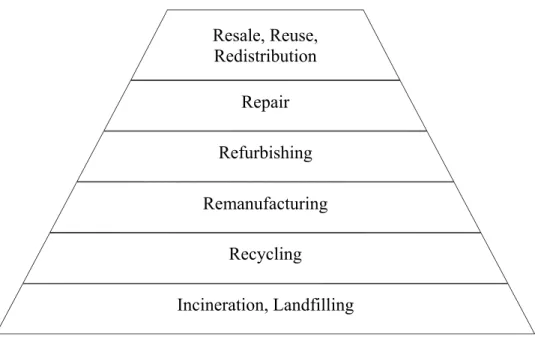
Resale, Reuse, Redistribution Repair Refurbishing Remanufacturing Recycling Incineration, Landfilling 1.3.2. How?

Now I will investigate the how question: How can be realized a reverse logistics system? I use to answer this question the paper of Thierry et al. (1995). This process consists of eight steps: direct reuse, repair, refurbishing, remanufacturing, cannibalization, recycling, incineration and landfilling. Figure 1 shows the connection between the elements of reverse logistics activities.

Direct reuse: the physical and quality property of products is unchangeable in the reverse logistics process.

Repair: The product will be transformed, and after this transformation (repair) the product can be used or sold, as a new product. Repair can occur at the user or in a repair shop. Under transformation I understand a change of parts, but other modules or elements of the product are intact.

Figure 2: Hierarchical connection of reverse logistics activities, Source: de Brito – Dekker (2002)

Refurbishing: Refurbished products are dismantled into modules, and then they assembled under less rigorous quality. There are repaired only the defective modules, so the lifespan of

Remanufacturing: From remanufactured products we wait as good quality as a new product. Remanufacturing is more than refurbishing, because all modules and parts are rigorously inspected before use process. Defective modules and parts are totally exchanged in the remanufacturing process.

Cannibalization: In this reuse process all of the returned products are dismantled, and there is a rigorous quality inspection. The regained parts and modules are reused in repair, refurbishing, and remanufacturing activities.

Recycling: The product loses the original function in this reuse method. The objective of recycling is to recover all usable material. If the quality of recovered materials is appropriate, then they can be used for manufacturing of new products.

Incineration and landfilling: These two categories belong to the waste management. Both activities must fill rigorous requirements. Economic advantages can be gained from incineration, if the rising energy is reused.

The above-mentioned fields are summarized in a pyramid in figure 2. This pyramid creates a close connection between reverse logistics and environmental protection. The levels shows which logistic activities promote the protection of environment. Some of the materials and wastes, as products of reverse logistics, can be handled with activities at the bottom of pyramid. The objective of a reverse logistics system is to introduce activities at the top of pyramid. The question is now, if the objective is reuse or reduction of resources, then the pyramid is why not broad at the top. The ideal situation would be an inverse pyramid, but reuse is nowadays not so general.

1.3.3. What?

The next question deals with the quality of the returned products in reverse logistics. In this case the assortment of returned products is examined: which factors damage the possibility of reuse, and how will the consumer use the reused products.

amortization of the products, which make more difficult the reuse. A typical example is electronic items, where the technical progress supersedes functioning, but obsolete products. The way of use of products influences the reuse. It depends on place, intensity, and duration of use, which determine a later remanufacturing. The collected items can be distinguished whether they originate from communal or industrial consumption. (E.g. because of transportation, handling, or quantity.) Here must be mentioned packaging materials, spare parts, or public goods.

1.3.4. Who?

The fourth important field is the identification of participants in the reverse logistics. In this context I distinguish the participants of traditional value chain, and of reverse processes, and other participants, e.g. charity organizations. Till some of interested persons organize the reverse process, others deal with the practical realization. It is very important to coordinate the connection between supply chains. One of the coordination mechanisms is a reliable information flow. Necessary information for a successful functioning is summarized in paper of Thierry et al. (1995). On the basis of this article there are four groups:

- Information about product assortment, i.e. about materials, their combination, quality, value, hazard, and possibility of manufacturing (analyzes).

- Information about extent and uncertainty of reverse processes:

• Warranty – quantity and quality of returned products is uncertain, necessary repair activities are hard to plan.

• Off-lease and off-rent contracts – they can be estimated very well in quantity and in time, but to estimate the quality is hard.

• Voluntary buy-back – it depends on the possibility of manufacturer. The advantage of this solution is that it insures inexpensive resources for manufacturing and repair. Waste disposal costs decrease at the consumer, and it makes possible for the manufacturer to sell new products.

used products. Reuse can be made by the manufacturer, but other firms can realize the reuse inside and outside supply chain.

- Information about collection of used products and waste disposal. The examination includes organizations involved in the process, obstacles occurred, quantity of returned products, and cost-benefit analyzes.

1.4. Stakeholders of reverse logistics

Participants of reverse logistics can be approached in another way. A theoretical background is supplied in paper of Carter and Ellram (1998), in which there are internal and external factors that influence reverse logistics.

In general, there are factors within organizations and between organizations, which are external factors. Internal factors belong interested persons inside of firms, steps for protection of environment, successful applied business ethics standards, and mainly those persons who are responsible for the environment friendly corporate philosophy. Also internal influences have the consumers, supplier, competitors, and government. These four elements are influenced also by the macro environment with social, political, and economic trends that touch reverse logistics indirectly.

The listed sectors have a different effect, and they have several interpretations. Among external factors governmental sector has a most determining influence. It can be accepted from environmental protection point of view, considering that environmental problems initiate most of the questions in the European Union. It must be remarked that law forces enterprises, till other competitors have to consider enterprise competitiveness in the same way. From this point of view a firm must meet the consumer need under keeping the environmental regulation of government. Without keeping governmental instruction an enterprise can not become competitive. There are two views about firm behavior.

Supply

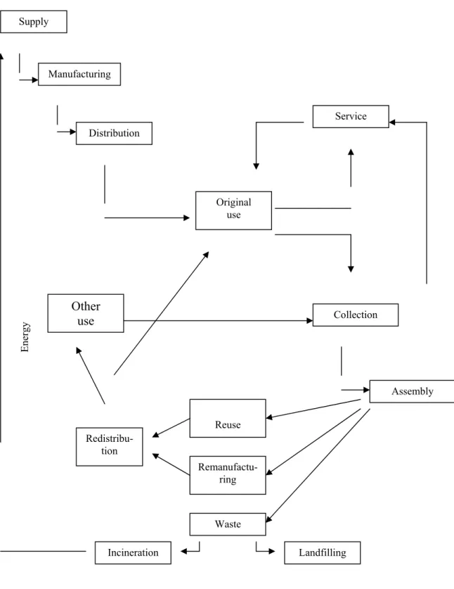
Figure 3: Connection of reverse logistics processes, Source: Kohut – Nagy (2004)

Importance of supply side is emphasized with the fact that colleagues of procurement departments purchase more used items, if the permanent good quality of reusable products is secured. Suppliers are responsible for collection and selection of used products generally, but

Reuse Original use Waste Remanufactu-ring Distribution Manufacturing Collection Assembly Service Incineration Landfilling Energy Redistribu-tion Other use

information. The quality of returned products has a risk potential for the supplier, so the integration between supplier and producer must be strengthened.

The role of the touched persons is an important internal factor. The owners of the firm can influence the functioning of reverse logistics system. They do not determine the activity of firms directly, but they can hinder it in a long range. Their assistance is a pre-requisite for a successful reverse process.

The role of management is similar to that of owners. Without any assistance of management a reverse logistics system can not be functioned effectively, but the functioning is made by the middle leaders of the firm. They must have good diplomatic and communication skills, and leading ability. They have the work to persuade the touched persons about the necessity of effective reverse logistics system.

Employees belong to the third group of stakeholders, who can help to introduce reverse logistics system through their contribution. Stimulation system can assist the efficiency. The above-mentioned external and internal factors have a synergy effect, i.e. both can make stronger their effect together. The consumer need must be considered, as a general rule. Also the internal and external interest must be considered. Without consideration of these interests a reverse logistics system can not be realized.

Figure 3 summarizes the examined connections about reverse logistics. I emphasize that the processes must be close. The figure presents a paper mill manufacturing process. Some of the important activities are neglected because of the simplicity.

1.5. Summary

All of the presented reverse logistics activities can not be found in a firm. There are a number of reasons, why. The available technology, great variety of products, and economic situation of firm influence the enterprise decision about applied reverse logistics system.

I do not investigate, what reverse logistics means for a specific product, and how a successful system could be introduced. These points requires further examinations, e.g. how a final

manufacturing process. At the same time, it is hard to follow all parts and modules from manufacturers to consumers, then through collection network to reuse fabrication. Nowadays there is no information system to follow the correct material flow along the supply chain. In some cases it is easy to model the reuse process, but in general it is not so. Some of the parts and modules can not reuse, and it is difficult to find an economic sector, where the reuse process can build up effectively. A typical example is computer, from which relatively a few parts can be recovered, and the reuse is economical only in a great extent.

These above-mentioned problems can be eliminated with a cooperation of different industrial sectors, and with a coordinated, reliable information flow between these sectors.

Our starting point was the protection of environment, which is stimulated by legal regulation and by enterprise responsibility. The firms are forced to meet governmental regulation, but a voluntary responsibility is influenced by the available financial sources. In a long range the costs and revenues must be analyzed. Environmental consciousness is not attractive without any economic gains.

The aim of this review is to give an introduction in the theory of reverse logistics systems. This chapter is a starting point to get acquainted with reuse processes, which raise a numbers of questions. This theoretical chapter gives a theoretical background, but the practical application of reverse logistics system needs further empirical investigations. The physical realization faces with technological difficulties, and on the other side the costs must be examined, as well. A successful reverse logistics along the supply chain can contribute to the reduction of loads of environment.

2. Economic Order Quantity Models in Reverse Logistics

Reverse logistics is an extension of logistics, which deals with handling and reuse of reusable used products withdrawn from production and consumption process. Such a reuse is e.g. recycling or repair of spare parts. An environmental conscious materials management and/or logistics can be achieved with reuse. It has an advantage from economic point of view, as reduction of environmental load through return of used items in the manufacturing process, but the exploitation of natural resources can be decreased with this reuse that saves the resources from extreme consumption for the future generation.

In this chapter I present three reverse logistic economic order quantity (EOQ). These models are not only shown, but extended, and I show that all of these models lead to the same mathematical structure named meta-model analyzed in the appendix. (Dobos-Richter (2000)) properties of meta-model are presented in the appendix. The following models are presented. The first reverse logistic (repair/reuse/recycling) model was first investigated by Schrady (1967) in an EOQ context. The paper has examined the cost savings of repair of high cost items at the U.S. Navy Aviation Supply Office in opposite to procurement. The condition of the basic model is that there are only procurement and several repair batches. The question is the lot sizes of procurement and repair.

Model of Nahmias and Rivera (1979) was the second lot sizing model. This model has extended the results of Schrady (1967) with finite repair rate, i.e. the repair process needs time. The repair rate is constant in time. The problem considers waste disposal of a reuse process. In the basic model Nahmias and Rivera (1979) have examined the case of one repair lot size. These investigations were supported by U.S. Air Force Systems Command.

The last model is model of Koh, Hwang, Sohn és Ko (2002). The authors of this paper analyze a model similar to that of Schrady (1967). Till the first two models examine a situation, where the new manufactured/procured and repaired products can arrive in a store, if the inventory level is equal to zero, in this model the recoverable inventory fulfils this property. This inventory strategy was named by Schrady (1967) as “continuous supplement” policy, but modeling of this situation was not published in his paper. The models of Schrady

(1967) and Nahmias and Rivera (1979) have applied an other inventory policy named “substitution”. Koh, Hwang, Sohn and Ko (2002) have not expressed the batch sizes, but they investigate two separate cases: number of purchasing batch is one, and repair batch is one. I show a new formulation of the model, which treats these two cases in a general model. Koh et al. (2002), examine an other model. In this model the reuse capacity is not greater than the demand rate. In my investigation I ignore this type of model.

There is a multi product generalization of EOQ-type reverse logistics models published by Mabini, Pintelon and Gelders (1998). They have extended the basic model of Schrady (1967) with capital budget restriction. The examined models have determined the lot sizes, but they have not taken into account that number of lots is integer, and the sensitivity of return process from parameters was not investigated.

After this brief overview I summarize the common conditions of these models.

1. The inventory holding policies are known in the models. It means that in an inventory cycle the inventory status is given and known in time.

2. The demand for new and recovered products is constant and deterministic in time. 3. The return rate of used items is constant and known in time. It is a similar condition to

that of last point.

4. The ordering costs of purchasing and setup costs of repair are known.

5. The inventory holding costs of recovered and new products and holding costs of used items waiting for repair are known.

6. There is no shortage in store of recovered and new products and store of returned items.

The first condition defines the inventory holding policy. The variables of these strategies must be determined in a model, i.e. the lot sizes for new and recovered products, number of batches for new and used products, and cycle time. The next four conditions are similar to that of traditional one product EOQ model, i.e. cost structure and demand process. The shortage situation is excluded with the last condition. Consideration of shortage is not a complicated mathematical problem, but the aim of this chapter is to give an introduction in the basic

2.1. A Reverse Logistics Model with Procurement and Repair

2.1.1. Introduction

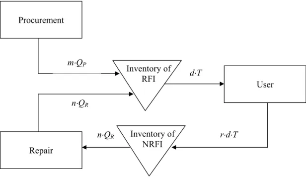
A deterministic EOQ-type inventory model for repairable items was first offered by Schrady (1967). This model can be seen as the first reverse logistics model. His model has examined the U.S. Naval Supply Systems Command stock holding problem with repairable items. The repairable items may be scrapped upon a failure, but the products are usually returned from the user to the overhaul and repair point. The repaired items are sent then to the ready-for-issue (RFI) inventory to await demand. Based on the feasibility of repair, the items not sent back are disposed of and they are replaced with new procured products. The returned and not repaired items are held in a second stock point, i.e. the inventory of non-ready-for-issue (NRFI) items are awaiting repair at the overhaul and repair point.

Schrady has offered to inventory holding policy to solve problem: the “continuous supplement” and “substitution” policies. To this last policy he has determined the optimal procurement and repair quantities. It was assumed that there are only one procurement quantity (batch size) and more than one repair quantities.

The aim of the paper is to analyze the introduced substitution policy in a general framework. In this generalization it is allowed a more than one procurement quantity. To solve the problem we use the meta-model. (See appendix.) Schrady has not investigated the integer solution for the repair batch number, it is examined now. We will show that the by Schrady offered solution can be improved in dependence on the recovery (return) rate.

The paper is organized as follows. The next section summarizes the parameters and functioning of the model. In section 3 we construct the inventory holding cost function of the model. Then analyzing the total average costs, we determine the optimal procurement/repair cycle. After eliminating the cycle time we have attained the model in dependence on procurement and repair batch numbers which leads to the meta-model investigated by the author, as well. Section 5 presents the basic model of Schrady with one procurement batch.

2.1.2. Parameters and functioning of the model

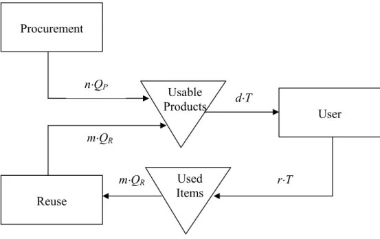
The system contains two inventories. The user’s demand can be satisfied from the RFI inventory. The demand of the user is constant in time. The RFI inventory is filled up with procured and repaired items. Shortage is not allowed in this stock point. The procurement and repair quantities are equal. From the user the repairable items are sent back to the overhaul and repair point with a constant rate. The repairable items are stored in the NRFI stock point waiting for repair. After repair products are seen as new and they are sent back to the RFI inventory. The material flow of the model is depicted in Figure 1. We define the variables and parameters as follows:

The decision variables of the model:

- QP procurement quantity,

- m number of procurements, m ≥ 1, integer, - QR repair batch size,

- n number of repair batches, n ≥ 1, integer, - T procurement/repair cycle time.

Parameters of the model:

- d demand rate, units per unit time,

- r the recovery rate, percent of the demand rate d, the scrap rate is 1-r, - AP fixed procurement cost, per order,

- AR fixed repair batch induction cost, per batch,

- h1 RFI holding cost, per unit per time,

- h2 NRFI holding cost, per unit per time.

The following equalities show relations between the in- and outflows in the stocking points in a procurement/repair cycle.

T d r Q n T d Q n Q m R R P ⋅ ⋅ = ⋅ ⋅ = ⋅ + ⋅

Figure 1. Material flow of the model

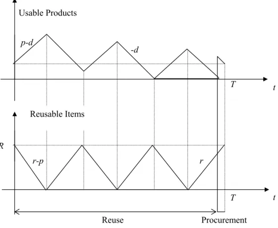
The offered “substitution” policy has the next property. The lead times for procurement and repair batches are disregarded, because in deterministic models its influence can be eliminated with a moving away. Let us assume that a procurement/repair cycle begins with induction of a repair cycle. The initial inventory level in NRFI stock point is reduced with a repair batch size. Then the remaining NRFI inventory decreases with a new repair batch, until it reaches the zero inventory level after supply in the RFI inventory. The time history of this policy is shown in Figure 3.

In the next two sections we construct the inventory holding and average inventory cost function of the model.

2.1.3. The inventory holding cost function

The holding costs of the model are calculated with the help of the inventory levels in time, as

n⋅QR d⋅T n⋅QR User Procurement Repair Inventory of RFI Inventory of NRFI m⋅QP r⋅d⋅T

Lemma 1.

Let the inventory holding costs for RFI items HRFI and for NRFI items HNRFI. Then the cost

functions have the next form:

2 1 2 1 2 2 P R RFI _d n Q h Q m d h H ⋅ ⋅ ⋅ + ⋅ ⋅ ⋅ = 2 2 2 1 2 R NRFI n Q r r n d h H ⋅      − ₊ ⋅ ⋅ ⋅ =

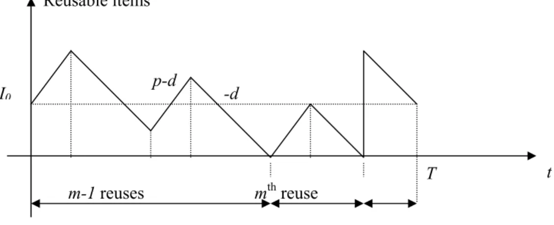
Proof. We will prove the second equation for the NRFI items, the first equation can be calculated in a similar way. Let us divide the area into n-1 triangles A, triangle C and n-1

rectangles B1, B2, ..., Bn-1. See Figure 3. The length of a repair cycle is

d Q_R . The area of a triangle A is d Q Q r R R⋅ ⋅ ⋅ 2 1

. The area of a rectangle Bi is equal to

(

)

d Q Q r i R R⋅ ⋅ − ⋅1 . The

maximum inventory level of NRFI items is n⋅Q_R −

(

n−1

)

⋅r⋅Q_R. The area of triangle C is

(

)

[

]

(

)

d r Q r n Q n Q r n Q n R R R R _⋅ ⋅ ⋅ − − ⋅ ⋅ ⋅ ⋅ − − ⋅ ⋅ 1 1 2 1 .

Let us now summarize the areas:

(

)

(

)

1 2 2

[

(

)

]

2 1 2 2 2 2 ₁ 2 1 2 1 Q n n r d r h i Q r d h Q r d h n H n _R i R R NFI = − ⋅ _⋅ ⋅ ⋅ + ⋅ − ⋅ ⋅

∑

+ _{⋅ ⋅} ⋅ ⋅ − − ⋅ − = .

After some elementary calculation we have the equation b).

Example 1. Let d = 1,000, r = 0.9, h1 = $ 750, h2 = $ 100. Then for this data the inventory

holding cost function is

2 2 2 2 900 1 100 11 10 1 R R P NRFI RFI H m Q n Q n Q H + = ⋅ ⋅ + ⋅ ⋅ + ⋅ ⋅

Figure 2. Inventory levels in the RFI and NRFI stock points (n = 3, m = 2)

Figure 3. The calculation of the inventory costs of NRFI items (m = 3)

NRFI inventory RFI inventory QR t t T T r⋅d -d QR QP Repair Procurement

(

n

)

r Q Q n⋅ − −1 ⋅ ⋅ Q A A t T r⋅ d B1 B2 C

2.1.4. Optimal procurement/repair cycle time

The fixed procurement and repair induction costs

R P n A A

m

F= ⋅ + ⋅

The total average costs are

(

)

T Q n r r n d h Q n d h Q m d h A n A m T H H F r m n Q Q T C R R P R P NFRI RFI R P 2 2 2 2 1 2 1 1 2 2 2 , , , , , ⋅       _⋅ − ₊ ⋅ ⋅ + ⋅ ⋅ ⋅ + ⋅ ⋅ ⋅ + ⋅ + ⋅ = = + + =

Let now use the equations the balance equations

(

) (

)

(

)

n T d r r n T Q m T d r r m T Q R P ⋅ ⋅ = ⋅ ⋅ − = , , 1 , ,

After substitution the economic order quantities we obtain a simpler cost function:

(

)

= ⋅ + ⋅ + ⋅ ⋅_ ⋅

(

−

)

⋅ +

(

+

)

⋅ ⋅ +h ⋅r⋅

(

−r

)

_ n r h h m r h d T T A n A m r m n T C P R ₁ 1 1 ₁ 2 , , , 2 ₂ 2 1 2 1 1

This function is convex in the cycle time then the necessary conditions of optimality are sufficient, as well. The optimal cycle time is

(

)

(

)

(

)

h r

(

r

)

n r h h m r h A n A m d r m n To P R − ⋅ ⋅ + ⋅ ⋅ + + ⋅ − ⋅ ⋅ + ⋅ ⋅ = 1 1 1 1 2 , , 2 2 2 1 2 1

(

)

= ⋅ ⋅

(

⋅ + ⋅

)

⋅_ ⋅

(

−

)

⋅ +

(

+

)

⋅ ⋅ +h ⋅r⋅

(

−r

)

_ n r h h m r h A n A m d r m n C , , 2 _{P R} 1 1 2 1 ₂ 1 2 1 2 1 2 or

(

)

( )

( )

C

( )

r m D

( )

r n E

( )

r m n r B n m r A d r m n C₂ , , = 2⋅ ⋅ ⋅ + ⋅ + ⋅ + ⋅ + where

( )

(

)

( )

(

)

( )

(

)

( )

(

)

( )

(

)

(

)

2 2 1 2 1 2 2 2 1 2 2 1 1 1 1 1 r h h A r h A r E , r r h A r D , r r h A r C , r h A r B , r h h A r A R P R P R P ⋅ + ⋅ + − ⋅ ⋅ = − ⋅ ⋅ ⋅ = − ⋅ ⋅ ⋅ = − ⋅ ⋅ = ⋅ + ⋅ =

Example 2. Let d = 1,000, r = 0.9, h1 = $ 200, h2 = $ 20, AP = $ 750, AR = $ 100. Then for

this data A

( )

0.9 =133,650,B

( )

0.9 =200,C

( )

0.9 =135,D

( )

0.9 =180,E

( )

0.9 =193,200

2.1.5. The basic model of Schrady

Schrady has investigated the case with only one procurement batch m = 1. The cost function of this model is

( )

(

)

( )

[

B

( )

r D

( )

r

]

n

[

C

( ) ( )

r E r

]

n r A d r , n , C r , n CS _{= 1 = 2⋅ ⋅ ⋅}1_{+ + ⋅ + +} 2

The optimal continuous solution for this case is

Lemma 2.

then

( )

r r h h h h A A r r r n R P o − ⋅ + + ⋅ ⋅ − = 1 1 2 1 2 1 _and

( )

(

)

(

)

(

)

        + ⋅ ⋅ +       − ⋅ + ⋅ ⋅ − ⋅ ⋅ = _{1 2 1 2} 1 1 2 r A h h r r h h A r d r , r n CS o _{P R} b) if

(

)

2 ₂

(

1

)

₁

(

1

)

2 0 2 1+ ⋅ − ⋅ ⋅ ⋅ − − ⋅ ⋅ − ≤ ⋅ h h r A h r r A h r A_{P R R} , then no

( )

r =1 _and

( )

(

n r ,r

)

d

(

A A

) (

[

h h

)

r h

(

r

)

h r

(

r

)

]

CS o _{= 2⋅ ⋅ P + R ⋅ + ⋅ + ⋅ 1− + ⋅ ⋅ 1−} 2 2 1 2 2 1

Proof. Let us investigate the function CS

( )

n,r _{. This function is convex in n. The minimal}

value of the repair batch number is

( )

_{( )}

( )

_{( )}

r r h h h h A A r r r D r B r A r n R P o − ⋅ + + ⋅ ⋅ − = + = 1 1 2 1 2 1 _.

After substitution the optimal value of n, we have the condition a) of the lemma. If this number is smaller then one, then the cost function is monotonously increasing for all n ≥ 1. This fact supports this condition b).

Remark 1. The function

( )

(

)

2 ₂

(

)

₁

(

)

2

2 1 h r A h r 1 r A h 1 r h A r F = _P ⋅ + ⋅ − _R⋅ ⋅ ⋅ − − _R⋅ ⋅ − is quadratic and monotonously increasing between zero and one. Value F

( )

0 =−A_R⋅h₁ is negative and

( )

1 A

(

h1 h2

)

F = _P⋅ + positive, so there exists a recovery rate r2 for which F

( )

r₂ =0. Then the

optimal batch number is equal to one for all r∈

[ ]

0,r₂ and it is greater than one for all

(

r₂,1

]

r∈ .

Remark 2. The solution for the batch number is not always integer for all r∈

(

r₂,1

]

. If value

( )

r

no _{is integer then the problem is solved. Let us now assume that n}o

( )

_{r is not integer. Let}

( )

r int

(

n

( )

r

)

the minimal integer not smaller than no

( )

r _{. The optimal integer solution can be determined}

from the following relation

( )

r

{

C

( )

n

( )

r C

(

n

( )

r

)

}

no S S

i =argmin , .

Theorem 1.

The optimal continuous the cycle time and order quantities of model of Schrady are

( )

(

) (

)

(

)

[ ]

(

)

(

)

(

]

       ∈ − ⋅ ⋅ + − ⋅ ⋅ ∈ − ⋅ ⋅ + ⋅ + + − ⋅ + ⋅ = 1 , 1 1 2 , 0 1 1 2 2 2 2 1 2 2 2 2 1 2 1 r r r r h r h A d r r r r h r h h r h A A d r T P R P o

( )

(

) (

)

(

) (

)

(

)

[ ]

(

)

(

)

(

]

       ∈ ⋅ + − ⋅ − ⋅ ⋅ ⋅ ∈ − ⋅ ⋅ + ⋅ + + − ⋅ − ⋅ + ⋅ ⋅ = 1 , 1 1 2 , 0 1 1 1 2 2 2 1 2 2 2 2 1 2 1 2 r r r h r h r A d r r r r h r h h r h r A A d r Q P R P o P and

( )

(

)

(

) (

)

(

)

[ ]

(

]

       ∈ + ⋅ ⋅ ∈ − ⋅ ⋅ + ⋅ + + − ⋅ ⋅ + ⋅ ⋅ = 1 , 2 , 0 1 1 2 2 2 1 2 2 2 2 1 2 1 2 r r h h A d r r r r h r h h r h r A A d r Q R R P o R

Proof. If r∈

[ ]

0,r₂ , i.e. the optimal repair batch number is one, then after substitution we have the optimal cycle and order quantities. To determine the other case, we use the following relation

( )

Substituting the optimal repair batch number and cycle time in balance equations, we get the results of the theorem.

Schrady in his paper has not analyzed those cases, for which the optimal batch number is even one. In this formulation we have shown that the solution supplied by Schrady

is limited to the case for r∈

(

r₂,1

]

. The method proposed in this paper has the same result for the economic order quantities, as obtained by Schrady. The optimal cycle time and economic order quantities for the integer batch number can be calculated with substitution and with some elementary operations.

Example 3. Let as in Ex. 2. d = 1,000, r = 0.9, h1 = $ 200, h2 = $ 20, AP = $ 750, AR = $ 100.

Then for this data the optimal continuous solution and the switching point r2 are r2 = 0.2316

and 4=18.754, =1, =0.628 , =62.828, o =30.151, S =$8,357. R o P o o o _{m T years Q Q C} n .

2.1.6. The optimal number of repair and procurement batches

To minimize the costs in dependence on the batch numbers we apply an auxiliary problem (meta-model). The problem is

(

)

( )

( )

C

( )

r m D

( )

r n E

( )

r min m n r B n m r A d r , n , m C₂ = 2⋅ ⋅ ⋅ + ⋅ + ⋅ + ⋅ + → subject to 1 1 ≥ ≥ , n

m . This problem was extensively studied in papers [1-5]. Based on the mentioned papers we examine the continuous solution of this model.

Theorem 2.

There are three cases of optimal solutions

(

n

( ) ( )

r ,m r

)

and the minimum cost expressions

( )

r

(i)

(

)

2 ₁

(

1

)

2 ₂

(

1

)

0 2 1+ ⋅ − ⋅ ⋅ − + ⋅ ⋅ ⋅ − < ⋅ h h r A h r A h r r A_{P R P}

( ) ( )

(

)

            + ⋅ − ⋅ = r h h h r r A A r m r n P R 2 1 1 1 , 1 ,

( )

{

(

)

1

[

1 2

]

}

3 r 2 d 1 r A h A r h r h C = ⋅ ⋅ − ⋅ _P⋅ + _R⋅ ⋅ ⋅ + (ii) 0≤ A_P⋅

(

h +h

)

⋅r2−A_R⋅h₁⋅

(

1−r

)

2 +A_P⋅h₂⋅r⋅

(

1−r

) (

≤ A_R +A_P

)

⋅h₂⋅r⋅

(

1−r

)

2 1

( ) ( )

(

n r ,m r

) ( )

= 1,1

( )

r d

(

A A

) (

[

h h

)

r h

(

r

)

h r

(

r

)

]

C = 2⋅ ⋅ _P + _R ⋅ + ⋅ 2 + ₁⋅ 1− 2 + ₂⋅ ⋅ 1− 2 1 3 (iii) A_P⋅

(

h +h

)

⋅r −A_R⋅h ⋅

(

1−r

)

2+A_P⋅h₂⋅r⋅

(

1−r

) (

> A_R +A_P

)

⋅h₂⋅r⋅

(

1−r

)

1 2 2 1

( ) ( )

(

)

            − ⋅ + + ⋅ − ⋅ = ,1 1 1 , 2 1 2 1 r r h h h h r r A A r m r n R P

( )

r d

{

r A

(

h h

)

A

(

r

)

[

h

(

r

)

h r

]

}

C₃ = 2⋅ ⋅ ⋅ _R⋅ ₁+ ₂ + _P⋅ 1− ⋅ ₁⋅ 1− + ₂⋅

It is easy to see that the three regions for the optimal solution in dependence on the return rate are not intersected. So we can calculate the values r1 and r2 (r1 < r2) for which either the

procurement batch or the repair batch is equal to one, but the other batch number is greater than one. Between these values both of the batch numbers are equal to one.

Example 4. Let as in Ex. 3. d = 1,000, h1 = $ 200, h2 = $ 20, AP = $ 750, AR = $ 100. Then

for this data r1 = 0.2341 and r2 = 0.2616. Let now substitute r = 0.9 in the optimal solution.

Then the optimal values are as calculated in Ex. 3.

The optimal procurement and repair batch sizes and the cycle times of the model are in dependence on the return rate:

(i) r∈

[

0,r₁

)

(

1 2

)

2 ) ( h r h r A d r T R + ⋅ ⋅ ⋅ = ,

( )

1 2 h A d r Q P P = ⋅ ,

( )

2 1 2 h r h r A d r Q R P _{⋅ +} ⋅ ⋅ = . (ii) r∈

[

r₁,r₂

]

(

)

[

r r

]

h r h A A d r T P R ⋅ + + − ⋅ + ⋅ = 2 2 2 1 1 2 ) ( ,

( )

(

) (

)

(

)

[

r r

]

h r h r A A d r Q P R P ⋅ + + − ⋅ − ⋅ + ⋅ = 2 2 2 1 2 1 1 2 ,

( )

(

)

(

)

[

r r

]

h r h r A A d r Q P R P ⋅ + + − ⋅ ⋅ + ⋅ = 2 2 2 1 2 1 2 . (iii) r∈

(

r₂,1

]

(

r

)

h r

(

r

)

h A d r T P − ⋅ ⋅ + − ⋅ ⋅ = 1 1 2 ) ( 2 2 1 ,

( )

₍

(

₎

)

r h r h r A d r Q P P _{⋅ − + ⋅} − ⋅ ⋅ = 2 1 1 1 2 ,

( )

2 1 2 h h A d r Q R P = ⋅ ₊ .

The proof is easy; we must substitute the continuous batch numbers in the order quantities and cycle times.

Example 5. Let as in Ex. 3. d = 1,000, r = 0.05, h1 = $ 200, h2 = $ 20, AP = $ 750, AR = $

100. Then for this data the minimal cost for the basic model: CS(0.05) = 17,589.8 and the minimal cost for the generalized model C(0.05) = 17,002.2. This means a cost saving of 3.5

percent of the total EOQ related costs.

2.1.7. Conclusion

In this paper we have reformulated and solved the model of Schrady. We have shown that for smaller recovery rate it gives a better solution if the procurement batch number is greater than one and on the basis of model of Schrady we can obtain a more effective solution for higher return rate. This result can be interpreted as a generalization of model of Schrady for the case of more than one procurement batch.

2.2. A Model with Purchasing and Finite Repair Rate: Substitution Policy

2.2.1. Introduction

The model of Nahmias and Rivera (1979) is a natural generalization of model of Schrady (1967). This model takes into account that repair process needs time, i.e. it depends on capacity.

The model and its solution will be presented in three steps. First I show the functioning of the repair-procurement process. After that the cost function will be constructed, and then the optimal decision variables are determined sequentially.

The presented model is an extension of basic model of Nahmias and Rivera (1979). The authors of this article have allowed only one procurement batch size. I allow in this chapter more than one procurement. As it will be shown, the number of repair and procurement batch sizes depends on the return rates.

2.2.2. Parameters and functioning of the model

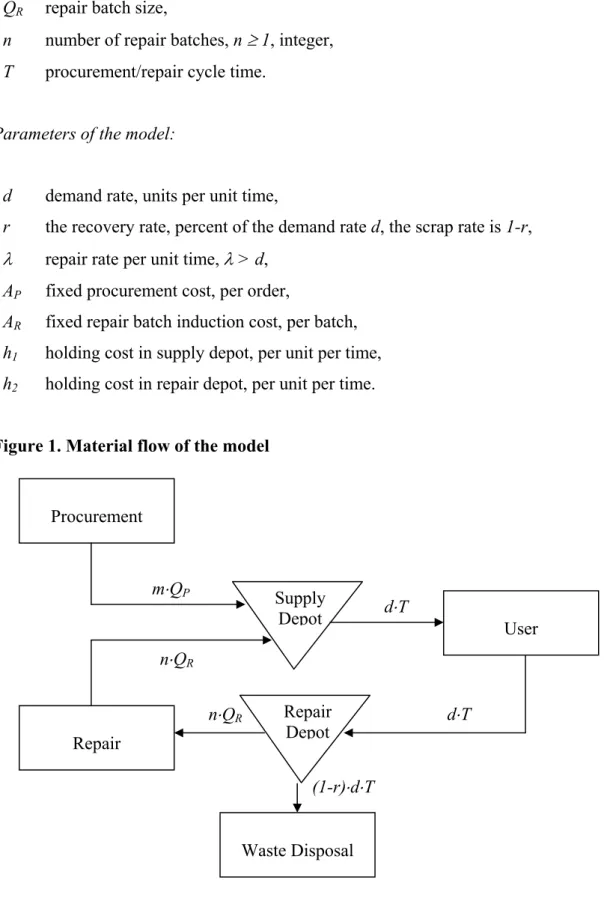
This inventory system contains two stocking points. The demand of the user is satisfied from supply depot. Demand is constant in time in a repair and procurement cycle. Supply depot is filled up from procurement and repair. Shortage is not allowed in this stocking point, so there are always new products. Procurement and repair batch sizes equal. User of spare parts sends back the used products in the repair depot with a constant return rate, till they are waiting for repair. In opposite to the model of Schrady (1967), the capacity of the overhaul department is finite. It is assumed that repair rate is greater than the demand rate. After repair the spare parts are sent back to the supply depot, and they are used as newly purchased products. The length of repair and purchasing lead times are constant, so they do not influence the decision variables. The material flow of the model is shown in figure 1. The used decision variables and parameters are similar to that of used by Schrady (1967). This circumstance makes it easier to compare these models.

- QP procurement quantity,

- m number of procurements, m ≥ 1, integer, - QR repair batch size,

- n number of repair batches, n ≥ 1, integer, - T procurement/repair cycle time.

Parameters of the model:

- d demand rate, units per unit time,

- r the recovery rate, percent of the demand rate d, the scrap rate is 1-r, - λ repair rate per unit time, λ > d,

- AP fixed procurement cost, per order,

- AR fixed repair batch induction cost, per batch,

- h1 holding cost in supply depot, per unit per time,

- h2 holding cost in repair depot, per unit per time.

Figure 1. Material flow of the model

(1-r)⋅d⋅T m⋅QP n⋅QR d⋅T n⋅QR User Procurement Repair Supply Depot Repair Depot d⋅T Waste Disposal

The following equalities show relations between the in- and outflows in the stocking points in a procurement/repair cycle. These equations make it possible to reduce the number of variables of the model.

T d r Q n T d Q n Q m R R P ⋅ ⋅ = ⋅ ⋅ = ⋅ + ⋅ (1)

This problem contains waste disposal, but it is not decision variable. The material flow and inventory status are illustrated in figures 1 and 2.

The proposed inventory holding strategy of this model is the substitution policy offered by Schrady (1967). Figure 2 presents the strategy where a cycle is begun with some repair batch sizes and then these lot sizes are followed by some procurement batches. The maximal inventory level is equal to 

     − λ d

Q_R 1 , which can be obtained from monographs of inventory controls. Used items are repaired at a rate of λ units per time, and r⋅d units are sent back to repair depot.

2.2.3. The inventory holding cost function

Inventory holding costs can be calculated by the help of figure 2. Lemma 1 summarizes this result.

Lemma 1.

Let inventory holding cost functions of supply and repair depot be A1 and A2. These two cost

functions can be written in the following form:

      − ⋅ ⋅ ⋅ ⋅ + ⋅ ⋅ ⋅ = λ d Q n d h Q m d h A _{P R} 1 2 2 2 1 2 1 1 , .       +       − ⋅ ⋅ ⋅ ⋅ = n r n Q d h A _R 1 1 2 2 2 2 2

Figure 2. Inventory levels in model of Nahmias és Rivera (n = 3, m = 2)

Proof. We will prove the second equation for the repair depot; the first equation can be calculated in a similar way. Let us divide the area into n triangles A, n-1 triangles B, triangle

D and n-1 rectangles C1, C2, ..., Cn-1. See Figure 3. The length of a repair cycle is λR Q . The area of a triangle A is       ₋ ⋅ ⋅ ⋅ λ λ d r Q_R 1 2 1 2

. The area of a triangle B is equal to

2 2 1 2      − ⋅ ⋅ ⋅ λ d r d Q_R .

The area of triangle D is

(

)

2

2 d QR m QP

r _{⋅ + ⋅}

⋅ . The area of a rectangle Ci is equal

to

(

)

d Q r

i_{⋅1− ⋅} R2 _.

Let us now summarize the areas:

QP λ- r⋅d -d Supply Depot t t T T r⋅d λ-d       − λ d Q_R 1 Repair Procurement Repair Depot

(

)

(

)

(

)

_∑

− = ⋅ ⋅ − ⋅ + + ⋅ + ⋅ ⋅ +       − ⋅ ⋅ ⋅ ⋅ − +       ₋ ⋅ ⋅ ⋅ ⋅ = 1 1 2 2 2 2 2 2 2 2 2 2 1 2 1 2 1 1 2 n i R P R R R i d Q r h Q m Q d r h d r d Q h n d r Q h n A λ λ λ .

After some elementary calculation we have the second equation.

Figure 3. The calculation of the inventory costs in repair depot (m = 3)

2.2.4. Optimal procurement/repair cycle time

The fixed procurement and repair induction costs are

R P n A A

m

F= ⋅ + ⋅

The total average costs are

(

)

T n r n Q d h d Q n d h Q m d h A n A m T A A F m n Q Q T C R R P R P R P       ₊       − ⋅ ⋅ ⋅ ⋅ +       − ⋅ ⋅ ⋅ ⋅ + ⋅ ⋅ ⋅ + ⋅ + ⋅ = = + + = 1 1 2 1 2 2 , , , , 2 2 2 2 1 2 1 2 1 λ .

The model leads to the following nonlinear optimization problem:

A B B C1 A A λ- r⋅d t T r⋅d D C2

(

)

        > > > ⋅ ⋅ = ⋅ ⋅ = ⋅ + ⋅ → integer. positive , , 0 , 0 , 0 , , min , , , , m n Q Q T T d r Q n T d Q n Q m m n Q Q T C R P R R P R P (P)

Let us now use the balance equations

(

)

n T d r Q m T d r Q R P ⋅ ⋅ = ⋅ ⋅ − = 1

After substitution the economic order quantities we obtain a simpler cost function:

(

)

(

) (

)

(

)

      − ⋅ ⋅ +       − ⋅ ⋅ + + − ⋅ ⋅ ⋅ + ⋅ + ⋅ = d h r r n r h h m r h T d T A n A m m n T C P R 1 _{1 1} 2 , , ₂ 2 2 1 2 1 1 _λ

This function is convex in the cycle time then the necessary conditions of optimality are sufficient, as well. The optimal cycle time is

(

)

(

)

h r

(

r

)

n d r h h m r h A n A m d To P R − ⋅ ⋅ + ⋅       − ⋅ ⋅ + + ⋅ − ⋅ ⋅ + ⋅ ⋅ = 1 1 1 1 1 2 2 2 2 1 2 1 _λ .

The simplified cost function is after substitution

(

)

(

)

(

) (

)

(

)

      − ⋅ ⋅ +       − ⋅ ⋅ + + − ⋅ ⋅ ⋅ + ⋅ ⋅ ⋅ = d h r r n r h h m r h A n A m d m n C , 2 _{P R} 1 1 ₂ 1 2 2 1 2 1 2 _λ or

(

)

( )

( )

C

( )

r m D

( )

r n E

( )

r m n r B n m r A d m n C₂ , = 2⋅ ⋅ ⋅ + ⋅ + ⋅ + ⋅ + , (2) where

( )

(

)

( )

(

)

( )

(

)

( )

(

)

( )

(

)

(

)

2 2 1 2 1 2 2 2 1 2 2 1 1 1 1 , 1 , 1 , 1 r d h h A r h A r E r r h A r D r r h A r C r h A r B r d h h A r A R P R P R P ⋅       − ⋅ + ⋅ + − ⋅ ⋅ = ⋅ − ⋅ ⋅ = ⋅ − ⋅ ⋅ = − ⋅ ⋅ = ⋅       − ⋅ + ⋅ = λ λ .

Problem (P) is simplified as an integer optimization model C2(n,m). Model (2) is the

meta-model of appendix.

2.2.5. The basic model of Nahmias and Rivera

Nahmias and Rivera have investigated the case with only one procurement batch m = 1. The cost function of this model is

( )

( )

( )

(

B

( )

r D

( )

r

)

n

(

C

( ) ( )

r E r

)

n r A d n C n CNR _{= 1, = 2⋅ ⋅ ⋅}1 _{+ + ⋅ + +} 2 .

The optimal continuous solution for this case is

Lemma 2.

The continuous solution of model of Nahmias and Rivera is

a) if

(

)

1 2 ₁

(

1

)

2 ₂ 1

(

1

)

0 2 1 ⋅ − ⋅ >      − ⋅ ⋅ − − ⋅ ⋅ − ⋅       − ⋅ + ⋅ h h d r A h r A h d r r A_{P R R} λ λ , then

(

)

      − ⋅ − ⋅ +       − ⋅ + ⋅ ⋅ − = λ λ d r r h h d h h A A r r n R P o 1 1 1 1 2 1 2 1 and

( )

(

)

(

)

              − ⋅ + ⋅ ⋅ +             − ⋅ − ⋅ + ⋅ ⋅ − ⋅ ⋅ = λ λ d h h A r d r r h h A r d n CNR o _{P 1 R 1} 1 1 2 _{1 2 1 2} ,