PURDUE UNIVERSITY GRADUATE SCHOOL Thesis/Dissertation Acceptance This is to certify that the thesis/dissertation prepared
By Entitled
For the degree of
Is approved by the final examining committee:
To the best of my knowledge and as understood by the student in the Thesis/Dissertation Agreement, Publication Delay, and Certification Disclaimer (Graduate School Form 32), this thesis/dissertation adheres to the provisions of Purdue University’s “Policy of Integrity in Research” and the use of copyright material.
Approved by Major Professor(s):
Approved by:
Head of the Departmental Graduate Program Date
Wenhan Huang
PARALLELIZED RAY CASTING VOLUME RENDERING AND 3D SEGMENTATION WITH COMBINATORIAL MAP
Master of Science in Electrical and Computer Engineering
Dr. Paul Salama Chair Dr. Maher Rizkalla Dr. Lauren Christopher Dr. Kenneth Dunn Dr. Paul Salama Dr. Brian King 4/25/2016
SEGMENTATION WITH COMBINATORIAL MAP
A Thesis
Submitted to the Faculty of
Purdue University by
Wenhan Huang
In Partial Fulfillment of the Requirements for the Degree
of
Master of Science in Electrical and Computer Engineering
May 2016 Purdue University Indianapolis, Indiana
ACKNOWLEDGMENTS
First, I would like to thank Dr. Paul Salama for guiding and helping me to com-plete this study.
I would like to thank my family, especially to my mother Yuwen Sun, my father Xiang Huang, my wife Qiaoqiao Wan, Kaka, Cindy, Ivan, and Pebbles for their spir-itual and financial support to complete this study.
To Dr. Kenneth W. Dunn for his support of this study.
To Dr. Lauren Christopher, Dr. Maher Rizkalla, Dr. Brian King, and Dr. Yaobin Chen for advice and guidance.
To Jerry Su for his contribution on Voxx 3.
TABLE OF CONTENTS Page LIST OF TABLES . . . v LIST OF FIGURES . . . vi SYMBOLS . . . viii ABBREVIATIONS . . . ix ABSTRACT . . . x 1 INTRODUCTION . . . 1
1.1 Introduction of Volume Rendering . . . 1
1.2 Volume Rendering and Scientific Visualization . . . 2
1.3 Ray Casting and Parallel Computing . . . 2
1.4 History of 3D Volume Rendering . . . 3
1.5 Introduction of Image Segmentation . . . 4
1.6 Segmentation Method . . . 5
1.7 Organization of the Thesis . . . 6
2 VOXX 3 . . . 8
2.1 Purpose and Background . . . 8
2.2 GPU Graphics Pipeline . . . 9
2.2.1 OpenGL . . . 9
2.2.2 Rendering Pipeline . . . 9
2.3 Architectural Design . . . 14
2.4 Decomposition Description . . . 16
2.4.1 OpenGL Rendering Module . . . 16
2.4.2 Color Look-up Table Module. . . 21
2.4.3 3D Stack Image Module . . . 22
Page
2.4.5 Image Capture Module and Movie Record Module . . . 26
2.4.6 Image Processing Function Module . . . 26
2.5 Contribution. . . 29
2.6 Result . . . 29
3 COMBINATORIAL MAPS AND 3D IMAGE SEGMENTATION . . . . 33
3.1 Combinatorial Map Definition . . . 35
3.2 Combinatorial Map Construction . . . 37
3.2.1 Complete Map (Level 0 map) . . . 37
3.2.2 Level 1 Map and Face Removal Operation . . . 38
3.2.3 Inclusion Tree . . . 38
3.2.4 Level 2 Map and Edge Removal Operation . . . 39
3.2.5 Level 3 Map and Vertex Removal Operation . . . 41
3.2.6 Encoding Method . . . 43
3.3 3D Segmentation with Combinatorial Map . . . 47
3.3.1 Segmentation Algorithm . . . 48
3.4 Result . . . 49
4 GPGPU AND NVIDIA FERMI ARCHITECTURE . . . 56
4.1 CUDA Programming Model . . . 57
4.2 CUDA Kernel . . . 59
4.3 GPU Architecture. . . 60
4.4 CUDA Kernel Optimization . . . 65
4.5 Result . . . 69
5 CONCLUSION AND FUTURE WORK . . . 71
LIST OF REFERENCES . . . 73
LIST OF TABLES
Table Page
3.1 Running Time Table of Combinatorial Map Based Image Segmentation 52
4.1 GPU Memory . . . 63
A.1 3-Sewn Operation Look-up Table . . . 78
A.2 2-Sewn Operation Look-up Table . . . 79
A.3 1-Sewn Operation Look-up Table . . . 80
LIST OF FIGURES
Figure Page
2.1 Diagram of the Rendering Pipeline. Dot Block are Programmable Stage. 10
2.2 A Triangle Strip. . . 12
2.3 A Triangle Fan. . . 13
2.4 Voxx 3 Software Module Decomposition. . . 15
2.5 Ray Casting. . . 16
2.6 Ray Casting into Normalized Coordinate. . . 18
2.7 Testing Axis Aligned Bounding Box and Ray Intersection. . . 20
2.8 Visualization of Color Look-up Table. . . 22
2.9 The Process of Ray Casting Rendering and Color Look Up. . . 23
2.10 User Input Parameter and Data Flow Chart in Voxx 3 . . . 24
2.11 Voxx 3 Rendering Result of Microscopy Image Dataset. . . 30
2.12 Palette of RGB Channel, Look-up Table Visualization. . . 30
2.13 Microscopy Image Dataset. . . 31
2.14 Microscopy Image Dataset with Different Parameter. . . 32
3.1 Elements Decomposition of a 3D Object to Extract Combinatorial Map. 35 3.2 Darts in i-sewn Relationship . . . 36
3.3 Elements Decomposition of A 3D Object to Extract Combinatorial Map. 37 3.4 2D Image with Inclusion Tree . . . 40
3.5 Fictive Edge Example . . . 41
3.6 Minimal Combinatorial Map Generation . . . 42
3.7 Combinatorial Map Encoding Matrix . . . 44
3.8 Dart Number Notation. . . 45
3.9 1-Sewn Direction . . . 46
Figure Page
3.11 Three Consecutive Microscopy Image with Segmentation Result. . . 54
3.12 Segmented Microscopy Image DataSet. . . 55
4.1 CUDA Programming Model . . . 59
4.2 CUDA Kernel Function . . . 60
4.3 Nvidia Fermi Architecture (Source: NVidia) . . . 61
4.4 Fermi Streaming Multiprocessor (Source: NVidia) . . . 62
4.5 Bank Conflict. . . 65
4.6 Thread Global Memory Access. . . 68
4.7 Combinatorial Map Encoding Image . . . 69 4.8 Running Time Comparison With CPU Algorithm and GPU Algorithm. 70
SYMBOLS
Vd Direction Vector (Point from Camera Location to Voxel Coordi-nate)
Vcoor Voxel Coordinate Vector Vcamera Camera Location Vector
Vstep Step Vector (Increment Distant Vector) Vscale Scale Vector
dt Period Coefficient
α Transparency Coefficient of Current Voxel Cs Color of Sample Voxel
Co Final Pixel Color Observed by the Viewer Sblock Number of Threads per Block
Nreg Number of Register per Block Nrpt Number of Register per Thread Ntmax Maximum Simultaneous Threads
Ndata Total Number of Data that Needs to be Processed Nblock Total Block Number
ABBREVIATIONS
TIFF Tagged Image File Format GPU Graphics Processing Unit CPU Central Processing Unit RAG Region Adjacency Graph OBG Oriented Boundary Graph CT Computer Tomography
PET Positron Emission Tomography MRI Magnetic Resonance Imaging n-D n-Dimension
GPGPU General-Purpose Graphics Processing Unit SIMD Single Instruction Multiple Data
CUDA Compute Unified Device Architecture SM Streaming Multiprocessor
API Application Programming Interface LD/ST Load and Store Unit
CC Computation Capability SFU Special Function Unit
ABSTRACT
Huang, Wenhan. M.S.E.C.E., Purdue University, May 2016. Parallelized Ray Casting Volume Rendering and 3D Segmentation with Combinatorial Map. Major Professor: Dr. Paul Salama.
Rapid development of digital technology has enabled the real-time volume ren-dering of scientific data, in particular large microscopy data sets. In general, volume rendering techniques project 3D discrete datasets onto 2D image planes, with the generated views being transparent and having designated color that is not necessarily ”real” color.
Volume rendering techniques initially require designating a processing method that assigns different colors and transparency coefficients to different regions. Then based on the ”viewer” and the dataset ”location”, the method will determine the final imaging effect. Current popular techniques includes ray casting, splatting, shear warp, and texture-based volume rendering. Of particular interest is ray casting as it permits the display of objects interior to a dataset as well as render complex objects such as skeleton and muscle. However, ray casting requires large memory and suffers from longer processing time. One way to address this is to parallelize its implemen-tation on programmable graphic processing hardware. This thesis proposes a GPU based ray casting algorithm that can render a 3D volume in real-time application.
In addition, to implementing volume rendering techniques on programmable graphic processing hardware to decrease execution times, 3D image segmentation techniques can also be utilized to increase execution speeds. In 3D image segmentation, the dataset is partitioned into smaller sized regions based on specific properties. By
us-ing a 3D segmentation method in volume renderus-ing applications, users can extract individual objects from within the 3D dataset for rendering and further analysis. This thesis proposes a 3D segmentation algorithm with combinatorial map that can be parallelized on graphic processing units.
1. INTRODUCTION
1.1 Introduction of Volume Rendering
The invention that has a significant influence on the history of technology develop-ment can be classified into two types. The first catalog includes the inventions like the television and the telephone, which changed the livelihood of human firstly and then changed the way of how people see the world. The another catalog does it reversely, like the Relativity and the Roentgen Ray. They first changed the way how people see this world and then changed the way how people live. Volume rendering technology should belong to the second type. The considerable importance of volume rendering is its application in scientific data visualization. One of its primary application is contributed from the rapid development of medical imaging like microscopy imaging, Computer Tomography (CT), and Magnetic Resonance Imaging (MRI), Moreover, volume rendering technology can be applied in geological exploration, weather analy-sis, molecular modeling and other scientific fields. Right now, volume rendering with 3D image data set has become a major research area in clinic and academy.
The 2D image generated by volume rendering algorithm are transparent, and the color is designated instead of its real color. Volume rendering initially requires clas-sifying processing method, which assigns different regions with different color and transparency coefficient. Then based on the viewer and the date set location, the algorithm will determine the final imaging effect. The current popular algorithm includes ray casting, splatting, shear warp, and texture-based volume rendering. Vol-ume rendering techniques are designed to display the object inside the dataset, so that it can render complex object located in the dataset like skeleton and muscle. However, the drawbacks of the algorithm are large memory requirement and longer
processing time, which makes this algorithm not appropriate for real-time process-ing. Therefore, the current studies focus on speed up the rendering by parallelizing rendering algorithms on programmable graphic processing hardware or preprocessing dataset to skip objects in the dataset.
1.2 Volume Rendering and Scientific Visualization
Scientific visualization is a technology and methodology of computing. It utilizes the knowledge in computer graphic, image processing, and computer vision to trans-form the symbolic and digital intrans-formation into geometry, allowing the researchers to observe the computation result. It can bring enormous advantages to support scien-tific productivity and the potential for scienscien-tific breakthrough [1].
Volume rendering is a sub-branch in scientific visualization. It is a technique used to generate a 2D projection image from a 3D data set. Compare to other scientific visualization technique, The ultimate goal of Volume rendering is to display the 3D detail on an imaging plane. For example, if a house is used as a 3D volume, inside the house, there are furniture, appliance, and other objects. When the users view the house from the outside, only the exterior appearance can be observed, and the layout of the room or the arrangement of objects are occluded; but if the house and the objects are semi-transparent, all the detail can be viewed at the same time. This rendering effect is what volume rendering technique wants to achieve.
1.3 Ray Casting and Parallel Computing
The ray casting rendering technique [2] is the most well-studied image based vol-ume rendering method, due to its high-quality result and capability to render trans-parent effect. The idea of ray casting algorithm is very similar to light transmission in the real world, but it is done reversely. In nature, a light source emits a cluster of light rays that pass through a transparent object. Some of the rays will fall into out
eye and image on our retina. In volume ray casting algorithm, rays are cast from the eye to an image plane, one per pixel, and find the intersection the objects blocking the path of each ray. A ray is terminated if no other object falls in its path. During the transmission in the object, color values are sampled at a certain interval along the rays.
The limitation of ray casting algorithm is its massive computation. For a 5123
image, it requires 134,217,728 arithmetic operations to generate each frame. Fortu-nately, the advantage of this algorithm is the parallel nature in volume rendering. Therefore, ray casting is studied on its acceleration on special rendering hardware. Before GPU became capable of handling this kind of task, rendering hardware like volumePro [3] is widely used in this field. Recent research tends to accelerate the volume rendering technique like ray casting on modern graphic processing unit.
In the 1990s, people started to realize the power of parallel processing and began to perform general purpose computing on the graphic processing unit (GPU) pro-grammable shader. With the development of hardware, GPU shader is capable to read randomly from video texture memory based on mathematical and logical com-putation [1]. This advancement gives research opportunity to parallel any algorithms such as ray casting and significantly improved the rendering speeding of such method.
1.4 History of 3D Volume Rendering
In the 1970s, The first of volume rendering technique is implemented at Mayo Clinic. Later in the 1980s, due to the advancement of image processing hardware and data manipulation technique, the algorithm of volume rendering can be implemented on the parallel processing system. The volume rendering algorithm is first parallelized at the University of North Carolina and Pixar. The work at Pixar was derived from the work of Ed Catamull, PhD, and Alvey Ray Smith, PhD at LucasFilms, which is
used to generate more realistic computer graphics for the movies. The 3D rendering work in 1990s are significantly contributed by the graph acceleration hardware de-veloped by Silicon Graphics at Mountain View, California. Software that dede-veloped at Silicon Graphics optimize its application on medical aspect using special texture mapping technique [4].
In the past, Voxel-based volume rendering software like VolumePro were usually run on very expensive SGI workstations. In the 2000s, graphics processing units can achieve rendering speed at a lower cost. Therefore, many research organizations started to develop volume rendering software products. These software includes the Voreen developed by University of Munster, VolView developed by Kitware, and Voxx developed by Indiana University. These volume imaging programs are designed to use the commercial graphics processors like GeForce and Radeon. However, these volume rendering software do not fully unitize the capability of GPU to perform 3D image processing. Consequently, the new version of Voxx can perform some real-time image processing algorithms like filtering, image registration, and segmentation during rendering.
1.5 Introduction of Image Segmentation
Image Segmentation is a subtopic of the field of Computer Vision, which deals with the partition of a digital image into multiple segmentation. In particular, The goal of this image processing technique is to cluster pixels into salient image regions based on the characteristic. Through simplify the region or change the representation of an image, it transfers the original image into something that is easier to recognize by the computer or human eyes for further analysis. The segmentation algorithm is usually a middle step of an image processing algorithm such as object detection, recognition, image compression, and occlusion boundary estimation. Therefore, segmentation technique has a wide application in the vast field of Artificial Intelligence.
1.6 Segmentation Method
Based on application, there are many different approaches to performing image segmentation. Some popular methods are listed below.
Threholding
Thresholding method is one of the most popular segmentation algorithms due to its idea simplicity and fast speed. A typical thresholding segmentation algorithm uses a threshold value to convert a gray-scale image into a binary image. This method relies on selecting the appropriate threshold value. Since its advantage in processing speed, this approach is implemented in many image processing software.
Edge Detection
Edge detection algorithm uses the sharp pixel intensity adjustment at the region boundaries to classify different objects. In edge-based segmentation algorithm, a sharpen filter is applied to the image, which is finding the derivative of a 2D signal in mathematics. The pixels that are not separated by an edge are classified into the same region. The output edge image generated by the sharpen filter are usually rough edges, which means the edge is too wide to distinguish the region. Some edge thinning methods are applied to the edge image.
Region-Merging
Region-Merging segmentation compare every pixel inside a image with its neigh-bors using some merging criterion. Methods rely mainly on the assumption that the neighboring pixels within one region have similar features. The common procedure is to compare each pixel with its neighbors. If a similarity criterion is satisfied, the pixel will be set to the cluster as one or more of its neighbors. The selection of the similarity criterion is significant due to the results are influenced by noise.
Watershed
Watershed segmentation uses the gradient magnitude in an image as the separate line between different region, which is called as the region boundary lines and water-shed lines. To find the line in an edge image, the algorithm traces the pixel values with the highest gradient value. Then assume water is added into the image and pixels that belong to the same catch basin form a segment.
1.7 Organization of the Thesis
This thesis is organized as follows. The first part (chapter 3) describes Voxx 3, a retime volume rendering software for PC. Voxx implements the ray-casting al-gorithm with parallel voxel by voxel sampling. The software can render more than 1000 512×512 TIFF images with 500 samples per ray at 30 frames per second using graphics processing units (GPU) pipeline. In this thesis, the software architecture is discussed, which focusing on the software decomposition, OpenGL rendering algo-rithm, sampling method, and user input parameter. Then several features of Voxx 3, such as a palette module that allows user modify rendering result, the image and video capture module, and the image processing algorithms module are presented.
The second part (chapter 4) presents an algorithm to extract a topological model for a given 3D image that represents both geometrical and topological information. The calculation of the minimal topological map of a 3D image occurs in three stages. The output of each stage is the input of next stage. The outcome of each stage represents the intervoxel boundary information of surface elements, edge elements, and vertex elements correspondingly. The combinatorial map is the last stage in the hierarchy. In the second section, the definition of the combinatorial map and its applications and encoding method is given. Then a sequential algorithm that extracts the map of a given image in O(n3) time and a discussion about how to use this map
The last part (chapter 5) discusses the background knowledge of GPU algorithms based on CUDA. GPUs are widely used in image processing application. This section reviews NVidia Fermi GPU architecture, CUDA programming model, and CUDA Kernel optimization scheme. Finally, the combinatorial map extraction algorithm is modified and optimized for the general CUDA kernel.
2. VOXX 3
2.1 Purpose and Background
Volume rendering has wide application in scientific data visualization, especially in medical imaging. Medical images obtained via X-ray Computer Tomography (CT), Positron Emission Tomography (PET), Magnetic Resonance Imaging (MRI) and Mi-croscopy are usually composed of stacks of images T different depths or time points. Therefore, constructing of volume view instead of multiple single 2D views is crucial for researchers to analyze data, extract information, as well as helping physicians in performing diagnosis. Thus, the utility of volume rendering software is significant.
Ray casting [2] is very popular in volume rendering due to its conceptual simplicity and high-quality result. However ray casting rendering algorithms require much com-putation for each ray resulting in longer times to generate every frame. The compu-tation requirements make ray casting not practical in real-time rendering using serial computation. In order to improve rendering speed, one approach optimizing tech-niques that involve preprocessing the dataset are used to address the problem [5–7]. One approach involves skipping voxels or regions can be skipped during rendering. This technique requires repeated preprocessing after changing rendering parameters such as the voxel transparency coefficient. This technique also requires extra memory to store preprocessed dataset. Alternatively, [8, 9] described preprocessing methods that utilize segmented object rendering and iso-surface rendering, while [10] proposed an object order algorithm that terminates ray earlier in order to speed up rendering.
Moreover, special hardware that is designed for accelerating ray casting algorithms has been used to render volume [3, 11–13]. Sampling and composting in the dataset
are performed on optimized hardware increase the rendering speed. [14] proposed us-ing texture mappus-ing hardware like Silicon Graphics RealityEngine to render volume data. The dataset is stored in 3D texture memory, and samples are extracted from texture planes parallel to the image plane. This approach requires customers pur-chase expensive hardware. Instead of using specially designed hardware, a graphical processing unit (GPU) accelerated real-time rendering software, Voxx 3, is proposed in this thesis. Voxx 3 samples volume data that are stored in GPU texture mem-ory using direction gradients that calculated from texture coordinates and camera coordinates.
2.2 GPU Graphics Pipeline
2.2.1 OpenGL
OpenGL is a cross-platform and cross-language application programming interface that operates graphic processing unit to render a real-time 2D image on the computer screen. It has wide applications in game development, CAD, and data visualization. OpenGL started as a cross-platform standardization developed by Silicon Graphic Inc for their workstations in the 1990s. Until the late 1990s, OpenGL is accepted by the massive developer and then it become a standard graphic library for operating OpenGL graphic processing unit in PC [15].
2.2.2 Rendering Pipeline
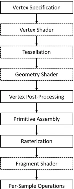
GPU rendering pipeline performs a series of processing stages in order. In the pipeline, The output of one stage is the input of the next stage. In Figure 2.1, vertex data are processed through the pipeline and the result are written into the screen buffer.
Fig. 2.1.: Diagram of the Rendering Pipeline. Dot Block are Programmable Stage.
Vertex Specification
In the vertex specification stage, a list of vertices with information like vertex location in 3D space, corresponding texture coordinate, plotting index, and vertex color are send into the pipeline. Generally speaking, the graphic pipeline starts with the 3D model; this model can be a 3D game character designed used modeling
software, or the vertices generated by a laser scanner. These vertices, which define the approximate boundary of objects, are stored in the GPU buffer such as Vertex Array Objects and Vertex Buffer Objects. In this step, transformation operation like rotation, scaling, translation can be applied to the vertices.
Vertex Shader
The process of GPU rendering pipeline begins with loading vertex attributes that stored in Vertex Array Objects or Vertex Buffer Objects and passing through the vertex shader. If a user defined vertex shader is not provided, GPU pipeline will pass vertices into a default shader. In this shader, GPU calculates the projected position of each vertex in array buffer and mapping them into screen space. Color or texture coordinates also can be modified based on the users’ demand.
Tessellation Shader
Tessellation shader is an optional stage in the GPU rendering pipeline. Until this stage, vertices can be operated using the vertex shader. Even though vertex shader is powerful, it still has a limitation, which is incapable of creating new primitives. To solve this problem, tessellation shader adds a new primitives types to the existed vertex array, called the patch. A patch is a primitive with vertices that defined by the user. The tessellation shader divides a patch into vertices and forms a triangle mesh.
The processing of tessellation consists of three stages, which are tessellation control shader, tessellation primitive generator, and tessellation evaluation shader. The first stage and last stage are programmable; the middle one is a fixed function stage [16]. The tessellation control shader determines the amount of tessellation for each primitive and performs designated transformation on the patch data.
Geometry Shader
The output vertices generated by the tessellation shader are then passed into an optional shader stage, called geometry shader. The geometry shader uses the single primitive as the input and transforms them into completely different primitives.
Vertex Post-Processing
After shader based vertex processing, the vertices are passed into a fixed post-processing stage. Depends on the projection method and view size, the projection matrix is calculated and primitives are clipped.
Primitive Assembly
In primitive assembly stage, GPU connects the vertices generated from previous stages. The GPU takes the vertices in the order specified by vertex array or user and segments them into triangles. Current rendering pipeline supports three methods [15]. 1) Take every three vertices inside vertex array buffer. This method requires 3×n vertices to generate n triangles.
2) Triangle strip: A triangle strip is a list of triangle vertices, which each triangle shares an edge with the previous triangle. an example is shown in Figure 2.2, A triangle strip or triangle fan are commonly used to compress the number of vertices that form an object.
3) Triangle fan: Triangle fans uses the same idea of triangle stripe. In a triangle fan, a vertex is shared with other two vertices where each three vertices will form a triangle. Figure 2.3 shows an example of triangle fans.
The indexes in Figure 2.2 and Figure 2.3 indicate the order when plotting each
Fig. 2.3.: A Triangle Fan.
vertex. In Figure 2.2, edge 2-3 is shared with the first triangle and second triangle. When GPU plots the triangles in the triangle strip, it takes the previous two vertices in the vertex array with a new vertex to generate each triangle. Compare to the first method, triangle strip requires n+ 2 vertex to represent n triangles. In Figure 2.3, Vertex 1 is shared with all the triangle. When plotting, GPU takes the first vertex and fetch two vertices in the vertex array to generate triangle.
Rasterization
Rasterization refers to the process of clip each primitive that fall outside the screen, break down the residual primitive into pixel size fragments, and assign pixel color to the fragments based on the vertex texture coordinate. In this step, GPU determines the location of the display window coordinate that occupied by the fragments and assign depth value as well as texture coordinate to each fragments. The generated fragments are sent into the next stage.
Fragment Shader
A fragment shader is the last programmable shader in rendering pipeline. The fragment shader operates fragment color based on user input, texture mapping, and lighting. The operation of on each pixel in the fragment runs independently from others. Therefore, fragment shader can provide the most impressive effect.
Per-Sample Operation
Per-sample operation stage contains a serial test for the fragment data generated by the fragment shader. The tests include Pixel ownership test, scissor test, stencil test, and depth test. These tests can be either turn on or disable. At last, the fragment data is written to the frame buffer.
2.3 Architectural Design
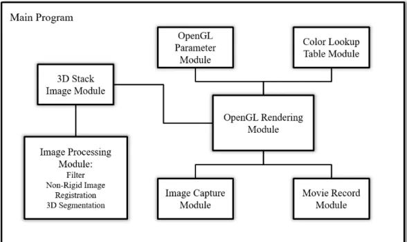
The Voxx 3 consists of several modules: a 3D stack image module, an OpenGL rendering module, an OpenGL parameter module, a color look-up table module, an image capture module and a movie record module. The interconnection among these modules provides the complete functionality of Voxx 3. Figure 2.4 describes the re-lationship between modules.
The 3D stack image module and the OpenGL rendering module are the core mod-ules of the program. They achieve the basic functionality of the program. The 3D stack image module decodes the input images and stores data in a 2D array in mem-ory, which is easier to use by the OpenGL rendering module. The OpenGL rendering module controls the GPU graphic pipeline, and responsible for displaying the ren-dering result on the screen. To change the renren-dering result based on user input like rotate or increase region intensity, user input parameter must be sent into OpenGL rendering module. Therefore, a OpenGL parameter module and color look-up table
module is designed to take user input. These two modules convert the user input to the parameter that can be used in OpenGL. Specifically, the OpenGL parameter module allows user to change blending method, modify volume boundary, and con-vert mouse movement into rotation angle. The look-up table module allows users to modify the color of rendering result, through modify the corresponding look-up table, where image voxels are used as indexes and final voxel values are find in look-up table. More detailed information can be found in section 2.4.5 and section 2.4.6.
In order to support function like region selection and improve rendering result, a image processing module is designed to support various image processing algorithm. The image processing module modifies voxel value that stored in 3D stack image module. Other features are implemented using the remaining modules. For instance, Image capture module and movie record module transfers pixel value in screen buffer back to memory and encodes it to images or movies for better demonstration purpose.
2.4 Decomposition Description
2.4.1 OpenGL Rendering Module
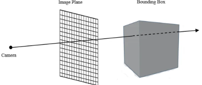
The rendering module utilizes volume ray casting, an image-based rendering tech-nique, to create a 3D perspective from a 3D texture data set.
Fig. 2.5.: Ray Casting.
Figure 2.5 shows a diagram that illustrate the whole process of ray casting algo-rithm. To set up the sense in openGL world coordinate, a camera, a image plane and a bounding box are created. Ray casting consists of three steps to generate result on image plane [2]:
1) Ray casting:
For every pixel on the screen, a ray is sent out, starting at the camera location, with a direction vector depending on the position of volumetric data location.
2) Sampling:
Along a ray cast through the volume, it is possible to sample the voxels for a certain interval. For the sample points that located between voxels, linear interpolation is applied to estimate voxel values from neighboring voxels.
3) Shading and compositing:
After interpolation, a pixel ( Pixel is used when dealing with 2D images and Voxel is used for 3D iamge) value is calculated for each sample point on the ray. Then based on the shading method, all the values of sample points are composited together using
a corresponding blending equation, resulting in a final pixel color. Eventually, this final pixel color is stored in the screen buffer and displayed on the screen.
Sampling in Normalized Dimensions
To represent a ray, direction vectors are obtained by calculating the casting di-rection of ray from the coordinate of the camera to the coordinate of image plane. Equation 2.1 shows how to calculate normalized ray casting direction Vdir. In the thesis, (x, y, z) represents the coordinate of each vector. In the equation, Vcamera represents the camera location in OpenGL world coordinate and Vcoor represents the image plane coordinate. Normalize indicates converting a vector into a unit vector.
Vdir=normalize(Vcoor−Vcamera) =
x/px2+y2+l2 y/px2+y2+l2 l/px2+y2+l2 (2.1)
After direction vector is obtained, the next step is acquired intersection point of casting ray and bounding box [17]. A ray can be represented using the camera coor-dinate and ray direction. Equation 2.2 shows the mathematical representation of a casting ray. In the equation, dt is a distance value that is used to calculate any point on the ray.
Vray =Vcamera+dt×Vdir (2.2)
All of the samples points that are used to calculate corresponding output pixel color fall along on this ray. The next step is to calculate step vector. This is necessary if the data set does not have same dimensions. Because to utilize date set in OpenGL, 3D data set must be transferred into texture memory. After images are transferred into texture memory, voxels are accessed using texture coordinates instead of its original indices. OpenGL texture coordinate is normalized, which means for a 3D
texture, its front left bottom corner is mapped to (0,0,0) and back top right corner is mapped to (1,1,1). Color information is retrieved from the voxels using these texture coordinates. As illustrated in Figure 2.6, it shows how to look into an object in the normalized coordinate. The small box represents the actual size of a 3D data set and the large box represents the box that is extended into the same dimension. Therefore, a step vectorVstep must be calculated to sample in the normalized coordinate.
Fig. 2.6.: Ray Casting into Normalized Coordinate.
Step vector should contain information about the direction and distance of the direction vector. Since different data sets may have different dimension, every compo-nent in step vector should increment different distance during sampling. To calculate step vector from direction vector, a weight valueCweight is given to every component in the step vector based on its corresponding dimension. Cweight contains the weight coefficients for each coordinate. The equation 2.3 show how to calculate step vector. In the equation, dx, dy, dz indicates the corresponding dimension of a 3D stack image. max(dx, dy, dz) means to choose the maximum value between dx, dy, dz.
Cweight = max(dx, dy, dz)/(dx) max(dx, dy, dz)/(dy) max(dx, dy, dz)/(dz) (2.3)
Then this weight coefficients is multiply with Vdir to calculate the step vector as shown in equation 2.4.
Equation 2.5 gives the method to sample in the texture memory. Vcurrent repre-sent the current texture location. This value is calculated based on the intersection between ray and bounding box [17]. Vcoor next the the next texture coordinate that need to be sampled. For any given interval dt, sampled voxels in the texture are saved and blended using the method purposed in next section.
Vcoor next =Vcurrent+dt×Vstep (2.5)
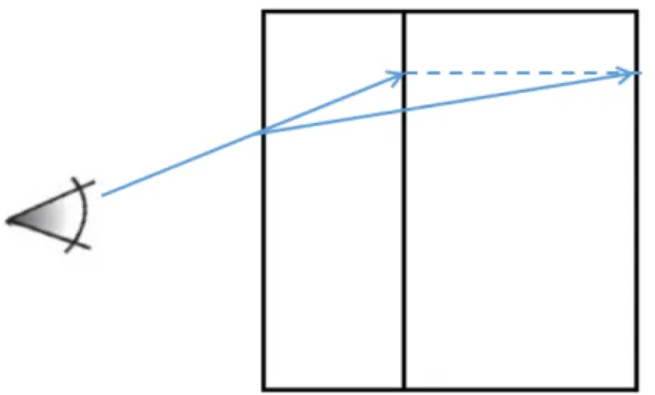
Ray and Bounding Box Intersection
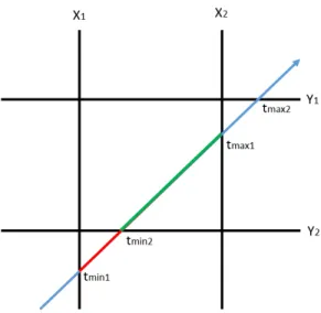
The middle step of a ray casting algorithm is to test the intersection between bounding box and each ray generated by the camera and image plane. The algorithm of performing ray and bounding box intersection is the one proposed in [18]. This algorithm tests the intersection between a ray and an axis aligned bounding box. An axis aligned bounding box indicates the faces of a bounding box must parallel to the coordinate plane. The algorithm treats the faces of the box as the planes that parallel to coordinate plane. The ray is clipped by the pair of parallel plane, and the portion inside the box intersected the box.
Figure 2.7 shows an example of testing intersection points between a ray and an axis aligned bounding box. It is easy to find the intersection point tmin1 of ray and
plane X1 and intersection point tmax1 of ray and plane X2. Then, points tmin1 and tmax1 are further tested with plane Y1 and Y2. Since tmin1 is located outside of plane Y1, this point is replaced with tmin2. In the end, tmin2 and tmax1 are the intersection
points of the ray and bounding box. dt is calculated using (tmin2−Vcamera)/vdir.
Blending Methods
All the voxels along the ray need to be composed together to obtain a final output pixel color. The method of composing them together is called the blending function.
Fig. 2.7.: Testing Axis Aligned Bounding Box and Ray Intersection.
Voxx 3 currently supports three blending methods: maximum, mean, and alpha blending. These three different blending methods will generate different rendering results.
Maximum blending uses the maximum voxel value along the casting ray as the final pixel value, as given by equation 2.5. In equation 2.5, Cs and Co represents cur-rent sample voxel and the output sample voxel correspondingly. The naming method applies to equation 2.6 and 2.7.
Co = n
X
s=0
M ax(Cs, Co) (2.6)
Mean blending uses the mean value of all the sample points on the casting ray, mean blending method average all the sample points on the ray by adding up all the pixel value and divided by the number of sample point:
Co = 1 n n X s=0 Cs (2.7)
Alpha blending uses a transparency coefficient to compose multiple voxels to-gether. An object transparency represents the capability that light transmit through the object without being scattered. When light passes through an object, its wave length will be changed based on the property of the object. When it passes through multiple objects, this change will be accumulated. Therefore, the fundamental of alpha blending is to mix the color of the current voxel with the next voxel on the casting ray. It preserves some features from the current voxel and also includes with part of the features from the next voxel. The equation of alpha blending is given in equation 1.7. In the equation, theαvalue represents the transparency coefficient of a voxel. Cs+1 represents the next voxel value andCo represents the output pixel value.
Co = n−1 X
s=0
αsCs(1−αs+1) +αs+1Cs+1 (2.8)
2.4.2 Color Look-up Table Module
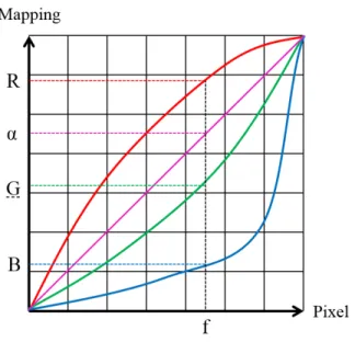
A color look-up table is a mapping mechanism that converts a range of pixel value into another range of colors. Look-up table is used to manipulate the image data. So the user can modify the mapping mechanism by modifying the corresponding look-up color to perform different look-up result. In general, look-up table is applied to a gray-scale image. The table converts gray-gray-scale images into color images. In Voxx 3, the color look-up table is used to increase the contrast of the region of the rendering im-age. The look-up table in Voxx 3 consists of three channel arrays of integers as shown in Figure 2.8. Original pixel color is treated as an address index to perform look-up in table. Figure 2.7 indicates how to find a corresponding color for a given value f. The red, green, blue, and pink curves in Figure 2.7 represent the output pixel values (For a 8 bits image, the range is from 0 to 255) in red, green, blue, and alpha channels.
For every sample on the casting ray, corresponding output from the sample value is found using look-up table and compose them using blending methods mentioned in
Fig. 2.8.: Visualization of Color Look-up Table.
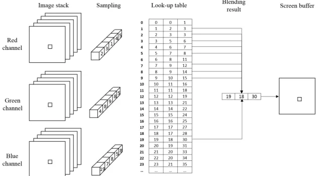
the previous section. In most color formats, the three channel arrays are either three primary colors, red, green and blue or HSI such as intensity, hue, and saturation. The procedure of color look-up and color composition is illustrated in Figure 2.8. As an example in Figure 2.9, one ray is sampled and the method is applied to other rays. On this ray, sample points 2,3,1,4,5 in red channel, 4,8,9,8,5 in green channel, and 19,7,8,5,8 in blue channel are obtained from dataset. These values are used as the index of color look-up table and the maximum blending method proposed in section 2.4.1, outcome (19, 18, 30) is the final pixel color that stored in pixel buffer.
2.4.3 3D Stack Image Module
The 3D stack image module in Voxx 3 provides the functionality of decoding input images and storing the decoded values. The module is implemented using an abstract class called threeDFiles. The threeDFiles class contains basic 3D image information like stack image dimension, image data pointer, and public functions that allow other modules to write and read these parameters. This class provides data set for the
Fig. 2.9.: The Process of Ray Casting Rendering and Color Look Up.
OpenGL rendering module, as well as image processing function module. In order to support different image formats, the threeDFiles class contains a virtual function to decode 3D stack images. This function is declared in threeDFiles class but without implementation. Therefore, this class cannot be instantiated, and it requires its sub-classes to implement decoding methods. Voxx 3 currently provides tiff3DFile inherited from threeDFiles to decode input TIFF images.
2.4.4 OpenGL Parameter Module
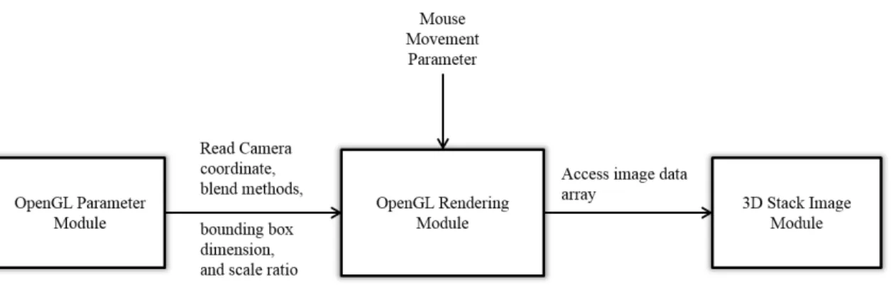
The functionality of OpenGL parameter module is passing user input and param-eters to OpenGL rendering module. It achieves interaction between users and Voxx 3. Voxx 3 allows user to rotate, zoom in, zoom out, scale, cut the object, and select different blending methods. The Figure 2.9 shows the data flow between different modules in Voxx 3. Once the parameter is changed, the updated values are sent to OpenGL rendering module to get new rendering result. OpenGL rendering module
uses this parameter to sample texture data in the 3D stack image module. In the parameter module, a transformation like rotate and scale are performed using matrix operations. In ray casting volume rendering, the rays generated from the camera and image plane are rotated instead of the bounding box. This is because testing intersection between ray and axis aligned bounding box is much faster than testing intersection between ray and bounding box in the arbitrary coordinate. Results of transformation are obtained using an Affine Transformation implemented in homo-geneous coordinate system [19].
Fig. 2.10.: User Input Parameter and Data Flow Chart in Voxx 3
An Affine Transformation is a linear mapping that transforms an original 3D co-ordinates to a new 3D coco-ordinates [19]. It preserves the linearity (all points on a line lie on the same line after transformation) and the vertex sequence (the order of each point on a line remains the same after transformation) of the original 3D images. In Voxx 3, a transformation is decomposed into rotation around x-axis and rotation around y-axis. Rotation operation, in 3D case, is to transform the voxel coordinates (x, y, z) by rotating the coordinates round a reference point with an specific angle. This can be achieved through matrix multiplication. Rotate transformation in 3D case can be expressed in matrix form as:
P0 =Rx(Θ)P = 1 0 0 0 0 cos(Θ) −sin(Θ) 0 0 sin(Θ) cos(Θ) 0 0 0 0 1 x y z α (2.9)
Rotation about the y-axis in 3D case can be expressed in matrix form as:
P0 =Ry(Θ)P = cos(Θ) 0 sin(Θ) 0 0 1 0 0 −sin(Θ) 0 cos(Θ) 0 0 0 0 1 x y z α (2.10)
In the equation 2.9 and 2.10, P represents either an original vertex coordinate or a vector. P’ represent its final coordinate after transformation. Θ is defined as the rotation angle. In Voxx 3, if user rotates the object for 30 degrees, a rotation matrix Ry(Θ) is multiplied with ray direction vector Vdir to obtain the final ray direction vector. As consequence, the intersection between ray and object is changed and so does the rendering result.
P0 =SP = Sx 0 0 0 0 Sy 0 0 0 0 Sz 0 0 0 0 1 x y z α (2.11)
Scaling enlarges or diminishes an object by a scale factor S. In equation 2.11, matrix S contains the scale factors Sx, Sy, Sz corresponding to X-axis, Y-axis, and Z-axis. In Voxx 3, if user enlarge or diminish an object, a scaling matrix is
mul-tiplied with the image plane. If scale factor S is larger than 1, then the object is diminished. This is because enlarging the image plane will decrease the density of rays correspondingly. More rays will miss the object and only the rays that pass the image plane center will hit the object. As the result, the object will looks smaller. In contract, if scale factor S is smaller than 1, then the object is enlarged.
Final Transformation is linear combination of rotation matrix and scale matrix can be expressed as:
P0 =SRy(Θ)Rx(Θ)P (2.12)
2.4.5 Image Capture Module and Movie Record Module
In Voxx 3, image capture module allows user to save screen display as images. Additionally, for better demonstration effect, the movie record module allows users to rotate the 3D object and record this 3D simulation. To obtain the real-time image or video, Voxx 3 is designed to transfer the pixel values in GPU screen buffer to CPU memory using direct memory access. To improve the capability and easier for user to access, the pixel values can be encoded into different format such as TIFF, PIC, PNG for images and MP4, MKV for videos.
2.4.6 Image Processing Function Module
Image processing function module contains three image processing algorithms in-cluding 2D/3D filter, Non-rigid image registration, and region-based 3D image seg-mentation. This module can visit data pointer in 3D image stack module, modifies voxels using various image processing algorithm and saves the data pointer back to 3D image stack module to improve rendering results or achieve functionality like re-gion selection. This module also contains image processing algorithms that running on GPU. These GPU functions are implemented using CUDA.
1) Filter:
Filter operation is widely used in image processing study. It can suppress or enhance a certain range of frequencies in the image to improve the quality of the image. Image filter can be applied either in frequency domain and spatial domain. To apply image filter in frequency domain, the transformation in frequency domain must be found and multiplied by the frequency function (usually a window function), then transform the result back into spatial domain. Processing image filter in the spatial domain is more widely used, first the inverse Fourier transform of filter function is found, and then convolve with the input image. The output image can be calculated as:
For 2D images: g(x, y) = M/2 X m=−M/2 M/2 X n=−M/2 h(m, n)f(x−m, y−n) (2.13) For 3D image: g(x, y, z) = M/2 X m=−M/2 M/2 X n=−M/2 M/2 X l=−M/2 h(m, n, l)f(x−m, y−n, z−l) (2.14)
2) Region Selecting function:
Region selection tools are designed to select regions on the 3D volume that rendered by Voxx 3 so that users can perform any edits, functions, or operations on them with-out affecting the unselected regions. Operations include analysis information or run image processing algorithm on a user-designated region. In order to select a regions inside of a 3D volume, a 3D segmentation algorithm are designed to partitions volume into multiple regions based on some criteria. Hence, user can select any region based on their demand.
In image processing, segmentation of an image is the process that partitions an image into multiple regions. The purpose of segmentation is to classify pixels with homogeneous properties (pixel values) into the same region for easier analysis and observation. These regions can be tread as different objects that allow users to ex-tract more information. There are many different segmentation algorithms, such as thresholding, clustering, edge detection and region based segmentation. Edge de-tection [20] method is a well-studied topic in image processing area. Many papers proposed very good segmentation results using this algorithm. It is very popular in image processing area. These algorithms are based on filter operation which is suit-able for parallel processing. Because parallel processing is much faster than sequential processing when dealing with large amounts of data, this advantage is significant in 3D image processing. However, the main drawback of edge detection algorithms is that edges are too rough to mark regions boundaries before edge thinning. And edge thinning technique may result in disconnected boundaries. Due to the intolerance of disconnect boundary when region selection (region selection usually uses a start pixel and perform breadth first search (BFS). BFS uses boundary as stop criteria. Therefore, disconnect boundary results in over selection). Therefore, In Voxx 3, re-gion based image segmentation is more stable than other algorithms. Rere-gion-based image segmentation requires a representation of region boundaries in the image. As in next chapter, a combinatorial map is very advantageous in representing adjacency relation among regions in a N-dimension image. This representation allows traversing between adjacent regions using different operations, such as find the left region of the current region or find the above region of the current region. In next section. This thesis will further discuss the basic definition of combinatorial map, the operation to construct a combinatorial map, and application in 3D segmentation.
2.5 Contribution
Previous Voxx development has focus on image registration and the rendering module. The present work is designed to provide many of the capabilities of the commercial volume rendering programs, including:
• support 12-bits and 16-bits TIFF images • support resampling methods and channel skip • modify graph-based color and opacity table editor • makes 3D movies(saved as AVI, MP4, TIFF series) • makes screen snapshot(saved as TIFF, PNG, JPG) • 2D and 3D filtering and 3D segmentation
2.6 Result
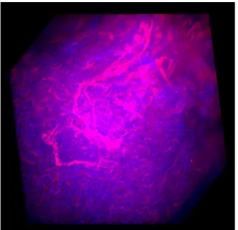
The software is tested on a PC with 64-bit Windows 8 operation system, an In-tel Core(TM) i7-4790 CPU @ 3.60GHz, NVIDIA GeForce GTX 760 Ti, and 16GB RAM. An example in Figure 2.1 is the rendering result of a stack image with di-mension (512×512×43). The picture is imaged using image capture module. It was rendered with 512×512 pixels, contains 262144 rays at 100 samples per ray.
Figure 2.10(b) shows the same image with rotation at angle 350◦ around x-axis and 200◦ around y-axis, maximum blending method, sample rate 200, and modified color look-up table.
The three palettes in Figure 2.11 correspond to red, green, and blue channel. In Figure 2.10(b). The X-axis of the palette represents the look-up address index from 0 to 255 for an 8-bits image. Y-axis represents output value from 0 to 255. The red,
(a) Result 1. (b) Result 2.
Fig. 2.11.: Voxx 3 Rendering Result of Microscopy Image Dataset.
(a) Red Channel. (b) Green Channel. (c) Blue Channel.
Fig. 2.12.: Palette of RGB Channel, Look-up Table Visualization.
green, blue (RGB) line in the image represent the corresponding output value from 0 to 255(8-bits image) in RGB channel. The pink line represents the alpha coefficient. The white line is the statistics histogram of pixel values in each channel. As shown in the red palette, red line and green line is modified based on user’s demand, blue line remain zero. As the rendering result, the color of blood vessel is changed to gold. Green color is added in blue channel, which resulting the cell color in the image changed to Aqua.
Fig. 2.13.: Microscopy Image Dataset.
Figure 2.12 is a different stack image rendering result tested on a PC with OS 64-bit Windows server 2008, an Intel E3-1225 @ 3.20GHz, NVIDIA Tesla c2075, and 32GB RAM and dataset. Rendering result is sampled from a stack image with dimen-sion (512×512×512). This volume is sampled at 500 samples per ray with maximum blending method.
Figure 2.13(a) is the same volume with maximum blending method but clipped into smaller dimension. Figure 2.13(b) is the same volume with blue channel removed and a bounding box.
(a) Alpha Rendering Result. (b) Maximum Rendering Result.
3. COMBINATORIAL MAPS AND 3D IMAGE
SEGMENTATION
A combinatorial map is a mathematical model that describes the intervoxel bound-ary and geometrical information. It encodes all the voxels, intervoxels and adjacent relation between them. Therefore, many studies have been made towards such a structure to represent 3D images due to its wide application in image segmentation, pattern matching, and other image processing algorithms. Both of these applications require an effective representation of image structure so that partition and merge can be easily operated [21–23]. In these types of application, different characters of target object need to be extracted in order to do further process. For segmentation algorithms, objects with same features, such as shape, size, color, and topological feature, need to be merged. Moreover, if images are stored in a form of boundaries and adjacency relations, some image processing algorithms can be done even without restoring the original image [24, 25]. Analysis of region structure is an important step before any 3D algorithms for computer vision. Therefore, development of an efficient and fast algorithm to extract topological structure is very crucial for image processing study.
In the early 1990’s, researchers studied many different approaches to represent 2D images using the topological structure. The most famous example is the Region Ad-jacency Graph (RAG) [26]. RAG describes images by vertex and edges that connect their neighboring region. Using this graph, it is really easy to find adjacent region for any given region using edges. However the major deficiency that RAG encountered is that RAG does not distinguish inclusion (there is no difference between adjacency and inclusion) and multiple adjacency relations [27, 28]. To solve this issue, W.G. Kropatsch proposed a dual-graph structure that consists of two multi-graph
describ-ing inclusion relation in 1994 [27, 28]. Addition to RAG, the pair of dual graphs has self-loops and multi-edge to indicate multiple adjacency relations. Dual graph solves the drawback of RAG, which trades increased space and time for adjacency infor-mation. As the result, any operation applied to a dual graph must be implemented twice, one for the prime graph and one for the dual graph. Dual graph structure is an excellent topological representation of an image. The idea can be easily extend to a higher dimension. Numerous research papers focus on this topic. Several studies based on 2D topological maps [29–32] proposed optimize methodologies to their ap-plication. Some of the models are also extend to 3D version [33,34]. The drawback of a dual graph is that it lack the explicit encoding of edges around vertices as existed in a combinatorial map.
In order to study the topological structure of a 3D model, researchers focus on Reeb graph, which represents the oriented structure of a 3D object. The Reeb graph describes the shape of the object but not its adjacency relationship [29]. Therefore, Reeb graph is not used in segmentation algorithm. Another approach is to use a combinatorial map [24, 35] or oriented boundary graph (OBG) [36, 37] to describe the topology structure of the image. The combinatorial map encodes all the inter-voxel elements and all adjacency information including regions Euler characteristic and Betti number using the basic element called dart. There are two ways to rep-resent a combinatorial map. One reprep-resentation is that using numbered segments to represent adjacent vertex and another representation is that using arrows instead. The oriented boundary graph uses nodes in the graph to represent regions of parti-tion and every oriented edge in the graph to represent the corresponding surfaces. OBG uses surface elements to represent surface adjacency relations. Compare to a combinatorial map, OBG has its advantages like simple extraction and low memory consumption. However, it does not describe the topological character of a region. In contrast, A combinatorial map is a useful model for preserving topological characters and describing space subdivision in a 3D image.
3.1 Combinatorial Map Definition
A combinatorial map is an intervoxel elements representation of n-D images, which is a mathematical model describing a subdivided object as a set of elements from ver-tices (0-Dimension elements denoted as 0-cell), edges (1-Dimension elements denoted as 1-cell), and faces (2-Dimension elements denoted as 2-cell). This map includes the adjacency relations among different cells that describe the topological information of the images. Two i-cells are defined as adjacent when they share a common (i-1)-cell. Figure 3.1 illustrates an example of decomposition of a 3D object to extract combi-natorial map. The combicombi-natorial map can be extracted by sequentially decomposing the volume of the object, faces of the volumes and edges of each face. In order to represent geometry information of n-cells, adjacent relation is encoded and denoted as β. Darts are represented as arrows and they are the basic elements to compose face, edge, and vertex as shown in Figure 3.1(d).
(a) 3D space subdivision. (b) volume decomposition.
(c) face decomposition. (d) edge decomposition.
Fig. 3.1.: Elements Decomposition of a 3D Object to Extract Combinatorial Map.
The initial definition of combinatorial map in N-dimension is given in [38]. Its definition is further extended to allow represent objects with boundaries. Based on the definition given in [24], a n-dimensional combinatorial map is a n-tuple M =
(D, β1, β2, ...βn). βn describes the relation between two i- dimension cells, where: 1. D is a finite set of darts;
2. β1 is a partial permutation on D;
3. ∀i2≤i≤n, βi is a partial involution on D;
4. ∀i0≤i≤n−2,∀j0≤i≤i−2, βi◦βi is a partial involution on D.
βn is called n-sewn operation and this encoding is used to find adjacent region in combinatorial map. Two darts d1 and d2 are i-sewn if they satisfy eitherβi(d1) =d2
or βi(d1) = d2. β1 represents relationship between two darts that share same face
and same volume, an example of 1-sewn relation is shown as the the pair of two blue darts in Figure 3.2. The permutation of darts consists an orbit, as the four blue darts presented in Figure 3.2. And β0 represents the reverse operation of β1. If β1(d1) = d2, thenβ0(d2) =d1. β2 represents relationship between two darts that share
same edge and same volume. This operation is used to find adjacent dart. The pair of two red darts in Figure 3.2 are in 2-sewn relationship. β3 represents relationship
between two darts that share same edge and same face. Traversing between the faces in the same region are through theβ1 and β3 operation. The pair of two green darts
are in 3-sewn relationship. In combinatorial map, vertex (0-cell) can be represented as< β21, β31 >(d), edge (1-cell) can be represented as< β2, β3 >(d), face (2-cell) can
be represented as < β1, β3 >(d).
3.2 Combinatorial Map Construction
3.2.1 Complete Map (Level 0 map)
The complete map is the starting point of combinatorial map extraction. This map includes all the intervoxel elements of a given image. For an1×n2×n3 labeled
image, its combinatorial map containsn1×n2×n3 dart cubes corresponding to every
voxel in the image. In Figure 3.3, figure (a) is a sample labeled image and Sub-figure (b) represents its corresponding level 0 complete map. In Figure 3.3(b), every voxel consists 24 darts, which results in 288 darts for a 4×3 image. Based on the definition of combinatorial map, the level 0 map is surrounded by an enclosing darts that describe its finite region. However, Figure 3.3(b) do not contain the finite region darts in order to make the map clear and understandable.
(a) 3D Space Subdivision. (b) Volume Decomposition.
(c) Face Decomposition. (d) Edge Decomposition.
3.2.2 Level 1 Map and Face Removal Operation
Level 1 map is extracted from level 0 map by removing face darts between two adjacency voxels that have the same value or similar property. The map excludes the internal surfels information of each region of a 3D image using face removal operation that presented in Algorithm 1 [24]. In order to extract level map 1 from level 0 map, the image is scanned and faces that need to be merged are removed. Face removal is processed by removing the 8 darts between the two voxels. Figure 3.3(c) shows level 1 map obtained from image the given in Figure 3.3(a). Algorithm 1 in next page gives the procedure of removing faces from a given 3D image. The algorithm takes a 3D image and generates a level 1 map. For each single face, it removes the permutation of dart d and orbit of β2(d).
3.2.3 Inclusion Tree
After face removal operation of a 3D combinatorial map, the generated level 1 map may lose volume connection information if the map contains two or more regions that one of the regions is surrounded by another region [38]. This kind of disconnec-tion is called volume disconnecdisconnec-tion. As the result, the combinatorial map will lose the topological information between these two regions. Therefore, a supplementary data structure is required to save connection information between different regions as shown in Figure 3.4(b).
An inclusion tree is designed to solve this situation. As shown in Figure 3.4, the inclusion tree on the right side includes the connection information of the image on the left. The root of the tree contains the boundary of stack image. Each node under the tree root represents a region corresponding to the regions in Figure 3.4(a). Different regions that share the same parent are saved as the child nodes of that parent node. Nodes in the tree contain boundary information or darts of a corresponding region. Algorithm 2 in the next page gives the procedure to generate inclusion tree structure.
Algorithm 1 Level 1 Map Extraction
Require: level 0 map M with dimension (n1 ∗n2∗n3)
for k = 0;k < n1;k+ + do
for j = 0;j < n2;j + + do
for i= 0;i < n3;i+ + do
if M(i, j, k) == M(i+1, j, k)then remove Orbit(d) and Orbit(β2(d))
end if
if M(i, j, k) == M(i, j+1, k)then remove Orbit(d) and Orbit(β2(d))
end if
if M(i, j, k) == M(i, j, k+1)then remove Orbit(d) and Orbit(β2(d))
end if end for end for end for
return level 1 map M
An inclusion tree is used to identify the region that a particular voxel belongs to. A tree traversal algorithm gives the procedure to search a region in the tree structure. The algorithm iteratively searches the tree level by level to identify a specific region.
3.2.4 Level 2 Map and Edge Removal Operation
Level 1 map represents the boundary information about the input 3D image. However, it still contains too much redundant information (darts), and is not efficient enough to describe the topological relationship of the image. To further minimize the map, adjacent faces that belongs to the same region are merged by removing edge
(a) Original Image. (b) Inclusion Tree.
Fig. 3.4.: 2D Image with Inclusion Tree
Algorithm 2 Inclusion Tree Generation
Require: Background Node RBG, Region List L for every R in region list L do
Node Rc =RBG while 1 do
for every subnode Rs in Rc do if R belongs to Rs then Rc = Rs continue end if end for insert R as subnode of Rc break end while end for
between them. To obtain the level 2 map, the whole images are scanned slice by slice and any edges that their degrees (the number of times of each distinct faces incident to this edge) are equal to two are also removed. During removal, some criteria must be applied in order to avoid removal of fictive edges.
(a) Fictive Edge. (b) Regular Edge
Fig. 3.5.: Fictive Edge Example
A fictive edge is an edge that its removal will result in disconnection of two faces. In Figure 3.5(a), the bold dart pair indicates a fictive edge. If this edge is removed, the relationship between two faces will be lost. In Figure 3.5(b), the bold dart indicates real edge, edges like this should be removed. Earlier study has presented Algorithm 3 [24] to determine if the edge has to be removed as shown below.
3.2.5 Level 3 Map and Vertex Removal Operation
The last construction of vertex removal operation is to removal every vertex that has two edges directly connect to it. Then for each dart exist on the map, the vertex removal operation trace through it along its direction and check if the degree of the vertex is equal to two, if true, the vertex will be removed. Figure 3.6(d) shows the corresponding level 3 map of Figure 3.6(a).
Algorithm 3 Edge Removal
Require: level 1 map M with dimension (n1 ∗n2∗n3)
for every dart d in level 1 map M do if β23(d)6=β32(d) then return; end if if β0(d)6=β2(d)andβ1(d)6=β2(d) then return; end if d0 =βd;d1 =β21(d);d2 =β20(d);d3 =β1(d); 1−sew(d0, d1); 1−sew(β3(d1), β3(d0)); 1−sew(d2, d3); 1−sew(β3(d2), β3(d3)); Removed, β2(d), β3(d), β23(d), end for
return level 2 map M
(a) Original Image. (b) Combinatorial Map
Fig. 3.6.: Minimal Combinatorial Map Generation
procedure that uses the cell operation proposed in previous sections. The algorithm takes labeled image and constructs combinatorial map level by level.
Algorithm 4 Combinatorial Map Extraction
Require: level 0 map M with dimension (n1 ∗n2∗n3)
for k = 0;k < n1;k+ + do
for j = 0;j < n2;j + + do
for i= 0;i < n3;i+ + do
if merge condition for f1(resp. f2, f3) then faceremoval(f1(resp. f2, f3))
end if
if local degree of e1(resp. e2, e3) = 2 then if e1(resp. e2, e3) is not fictive edge then
edgeremoval (e1(resp. e2, e3)) end if
end if
if local degree of v =2then vertexremoval(v)
end if end for end for end for
return level 1 map M
3.2.6 Encoding Method
A combinatorial map represents geometry information and boundary information of a labeled image. Different encoding methods are applied to the map depending on their applications. If only the geometry information of a given region is necessary but do not care about a voxel that belongs to a specific region, it is only necessary to use a hierarchical model. In this model, faces are represented as numbered seg-ments and edge are represented as oriented darts [39]. If an application requires both
information, [24] presents another solution to encode the combinatorial map. It re-quires a 3D matrix to represent all the intervoxel elements of a 3D labeled image, and uses 7 bits to represent the intervoxel elements between voxels as presented in Figure 3.7. For each element in a intervoxel matrix, it contains 3 bits for the front face, the top face, and the left face, 3 bits for the top front edge, the front left edge and the top left edge, 1 bit for the top left vertex. Figure 3.8 shows the intervoxel representation for one voxel. To represent the whole boundary for 3D image, it re-quires (n1+ 1)×(n2+ 1)×(n3+ 1) matrix to represent an1×n2×n3 image. [24] also
proposed the link between the darts of a topological map with triple (vertex, edge, face). Triple (f1.(i, j, k), e1.(i, j, k), v.(i, j, k)) is equal to d0 at voxel (i, j, k).
(a) Boundary elements. (b) Bit Representation
Fig. 3.7.: Combinatorial Map Encoding Matrix
An intervoxel matrix encoding method requires more memory space than the hi-erarchical model. But using intervoxel matrix gives user more flexibility to remove intervoxel elements (by clearing the corresponding bits in the intervoxel matrix) and retrieve voxel location. Algorithm 4 proposed in [24] gives a sequential method to extract a combinatorial map of a labeled 3D image. Simple removal and retrieve operation make the matrix very suitable for 3D segmentation application. It allows user to select a specific region in segmented 3D image stack to get information like volume and shape of that region.
(a) Dart Number. (b) Extend Dart Map.
Fig. 3.8.: Dart Number Notation.
The main drawback of an intervoxel matrix is that it cannot preserve fictive edge. This map loses face connection information during edge removal in level 2 map con-struction (this problem is discussed in section 3.2.4). Different encoding method can be applied to address this problem. Instead of using 7 bits to represent boundary information, and retrieve dart d based on a triple (vertex, edge, face), every dart and its direction (used to represent i-sewn operation) are encoded into the matrix. Using this encoding, 3 bits are used to represent each dart as shown in Figure 3.8(b). Using 1 bit to represent its existence on the map and 2 bits to represent its direction. Dur-ing initialization of the map, existence bit are set to 1 to represent the darts belongs to the map. To remove a dart, the existence bit is set to 0 and its corresponding direction bits are set to 3 (other direction values represent the vertex between two darts is removed) to represent its removal. It is certainly guaranteed that the dart cannot point to direction 4 because it is removed in level 2 map construction, as shown in Figure 3.3(b). Direction value equals to 0 indicates dart points to corresponding location 1 as shown in Figure 3.9; Direction value equals to 1 indicates dart points to corresponding location 2 and so on. Encoding direction value allows us to track and keep the fictive edges.