Poise: Balancing Thread-Level Parallelism and Memory System Performance in GPUs using Machine Learning

(1)

Edinburgh Research Explorer

Poise: Balancing Thread-Level Parallelism and Memory System

Performance in GPUs using Machine Learning

Citation for published version:

Dublish, S, Nagarajan, V & Topham, N 2019, Poise: Balancing Thread-Level Parallelism and Memory System Performance in GPUs using Machine Learning. in 2019 IEEE International Symposium on High Performance Computer Architecture (HPCA). Institute of Electrical and Electronics Engineers (IEEE), Washington, DC, USA, pp. 492-505, 25th IEEE International Symposium on High-Performance Computer Architecture, Washington D.C., United States, 16/02/19. https://doi.org/10.1109/HPCA.2019.00061 Digital Object Identifier (DOI):

10.1109/HPCA.2019.00061 Link:

Link to publication record in Edinburgh Research Explorer Document Version:

Peer reviewed version

Published In:

2019 IEEE International Symposium on High Performance Computer Architecture (HPCA)

General rights

Copyright for the publications made accessible via the Edinburgh Research Explorer is retained by the author(s) and / or other copyright owners and it is a condition of accessing these publications that users recognise and abide by the legal requirements associated with these rights.

Take down policy

The University of Edinburgh has made every reasonable effort to ensure that Edinburgh Research Explorer content complies with UK legislation. If you believe that the public display of this file breaches copyright please contact [email protected] providing details, and we will remove access to the work immediately and investigate your claim.

(2)

Poise: Balancing Thread-Level Parallelism and Memory System Performance in

GPUs using Machine Learning

Saumay Dublish, Vijay Nagarajan, Nigel Topham

University of Edinburgh

{saumay.dublish, vijay.nagarajan, nigel.topham}@ed.ac.uk

Abstract—GPUs employ a high degree of thread-level

paral-lelism (TLP) to hide the long latency of memory operations. However, the consequent increase in demand on the memory system causes pathological effects such as cache thrashing and bandwidth bottlenecks. As a result, high degrees of TLP can adversely affect system throughput. In this paper, we present

Poise, a novel approach for balancing TLP and memory system

performance in GPUs. Poise has two major components: a machine learning framework and a hardware inference engine. The machine learning framework comprises a regression model that is trained offline on a set of profiled kernels to learn best warp scheduling decisions. At runtime, the hardware inference engine uses the previously learned model to dynamically pre-dict best warp scheduling decisions for unseen applications. Therefore,Poisehelps in optimizing entirely new applications without posing any profiling, training or programming burden on the end-user. Across a set of benchmarks that were unseen during training,Poiseachieves a speedup of up to 2.94× and a harmonic mean speedup of 46.6%, over the baseline greedy-then-oldest warp scheduler.Poiseis extremely lightweight and incurs a minimal hardware overhead of around 41 bytes per SM. It also reduces the overall energy consumption by an average of 51.6%. Furthermore, Poise outperforms the prior state-of-the-art warp scheduler by an average of 15.1%. In effect,Poise solves a complex hardware optimization problem with consider-able accuracy and efficiency.

Keywords-warp scheduling; caches; machine learning

I. INTRODUCTION

For the better part of this decade, GPUs have been at the center of major advancements in areas ranging from Artificial Intelligence to Enterprise Computing. In such emerging applications, high degrees of thread-level parallelism (via multithreading) are normally required. However, the conse-quent increase in demand for memory resources gives rise to problems such as cache thrashing [22], [23] and bandwidth bottlenecks [10], [12], adversely affecting system throughput. Due to this tension between thread-level parallelism (TLP) and memory system performance, balancing the two properties to maximize system throughput poses a significant challenge.

To improve memory system performance, several warp scheduling techniques have been proposed that limit the degrees of multithreading [40], [41]. Subsequent proposals in-troduced additional mechanisms to not only improve memory system performance, but also maximize TLP. For instance, Li

et al.[35] proposed Priority-based Cache Allocation (PCAL),

where they classify warps into two categories, referred in this paper as follows. 1 Vital warps (N): A subset of maximum allowable warps that are permitted to participate

Maximum warps Cache thrashing W1 W1 L1 cache W2 W2 W3W3 W4W4 W1 W1 W2W2 W3W3 W4W4 (a) Maximum TLP W1 L1 cache W2 W3 W4 W1 W2 Vital warps Cache-polluting warps

X

(b) Reduced TLP Figure 1. Tuningvital warpsandcache-polluting warps

in multithreading, in order to maintain a sufficient degree of parallelism in the system. 2 Cache-polluting warps(p): A subset of vital warps that are permitted to make allocations and evictions in the private L1 data cache, in order to maintain good cache performance. We refer to this dual category of warps as awarp-tuple. Therefore, the above categorization, also illustrated in Fig. 1, provides a set of twoknobsthat can be used to tune TLP and memory system performance in order to maximize system throughput.

The Problem:How to find the best warp-tuples?Finding the best performing warp-tuples is a complex hardware optimization problem. This is because of the following two reasons. Firstly, traditional heuristic-based search techniques are prone to local optima in presence of multiple performance peaks, as is the case in GPUs [16], [17], thereby leading to sub-optimal solutions. Secondly, iterative search techniques are slow and expensive, particularly in hardware, due to the time spent in sampling to generate new iteration points. It is specially detrimental when the starting point is far from the solution, thereby requiring several iterations to converge. While PCAL poses an important optimization problem, their solution employs heuristic-based iterative search and suffers from the same limitations mentioned above (discussed in Section III). In our experiments, we observe that statically optimal solution performs up to 182% better than PCAL (discussed in Section VII), thereby suggesting considerable room for further improvement over PCAL. Therefore, the key goal of this paper is to find good warp-tuples, and to do so expeditiously in hardware.

Proposal: In this paper, we propose Poise, a novel ap-proach to balance TLP and memory system performance.

Poisecomprises two major components: a machine learning

framework and a hardware inference engine. The machine learning framework uses a simple regression model, that is trained offline on a set of profiled kernels using sample input-output pairs. Each of these input-input-output pairs comprise the

(3)

warp-tuple that resulted in the best performance for a kernel (as the output), and the corresponding set of architectural and application features (as the input). The input features are carefully chosen using a detailed analytical model. Thereafter, a regression model learns a mapping from the selected architectural and application features, to the chosen warp-tuple. The learned mapping is provided to the hardware via the compiler and can be used to optimize an entirely new application (as demonstrated in Section VII).

At runtime, the hardware inference engine samples the same set of input features and uses the previously learned mapping to dynamically predict best warp-tuples on a new application. To safeguard against statistical errors in prediction, the inference engine performs a local search in the vicinity of the prediction to find a better warp-tuple, if any. This adds resiliency toPoiseagainst minor statistical errors arising from the machine learning framework. In our experiments, we observe that the local search converges at a short distance from the initial prediction,i.e.,at an average offset of around one vital and one cache-polluting warp from the predicted warp-tuple (discussed in Section VII-G). This indicates good prediction accuracy and low overhead of local search. The final warp-tuple is fed to a modified warp scheduler, thereby balancing TLP and memory system performance.

Result: Across a set of benchmarks that were unseen during training,Poiseachieves a harmonic mean speedup of 46.6% (up to 2.94×) over the baseline greedy-then-oldest (GTO) warp scheduler that employs maximum number of warps.

Poiseincurs a minimal hardware overhead of around 41 bytes

per SM and reduces the energy consumption by an average of 51.6%. It also outperforms the prior state-of-the-art warp scheduler, PCAL, by an average of 15.1%. It is noteworthy that training is performed offline by the GPU vendor and done only once. Therefore, unlike profiling-based techniques,Poise

poses no additional training or profiling burden on the end-users to run new applications.

II. BACKGROUND A. GPU Computing

A typical CUDA program consists of multiple kernels. Kernels are organized into data-parallel blocks of computation called thread blocks. Each thread block consists of even smaller group of threads calledwarps. In hardware, GPUs consist of multiple execution units organized into a set of

Streaming Multiprocessors or SMs. Each SM consists of

a private L1 data cache and a shared L2 cache. SMs also comprise several read-only caches such as constant cache. Constant cache is typically used to perform repeated reads to the same memory location. In this study, we consider a baseline modeled on a modern GPU, comprising 32 SMs, 16 KB L1 data cache and 2.25 MB shared L2 cache. Each SM supports up to 1536 concurrent threads and up to 48 warps. There are 2 warp schedulers per SM, where each warp scheduler manages a maximum of 24 warps at any given time. The baseline parameters are summarized later in Table IIIb.

B. Supervised Learning

Supervised learning is a machine learning technique, which uses atraining setthat comprises sample input-output pairs, and constructs a mapping from the input to the output by analyzing the training data. The learned mapping represents prior knowledge, and is used to make predictions orinferences

about the output on entirely new input data.

Feature selection: The input variables that are used for training are often referred as thefeature vector. The accuracy of the model depends highly on the selection of the feature vector. While correlation techniques [5], [18] are often used for selecting a set of representative features, domain knowledge can be harnessed by constructing robust theoretical models [4], [39] to discover a reliable set of features (as shown in Section V-A). This can help reduce the dimensionality of the feature vector to truly representative features, thereby improving prediction accuracy. It also alleviates the black box nature of the model, thereby improving explainability.

Regression analysis: In this paper, we use Negative Bi-nomial regression from the family of Generalized Linear Models [13]. In this regression model, output follows a

negative binomial distribution. The learned mapping from the

input to the output is expressed through a set offeature weights, one for each corresponding input in the feature vector. The logarithm of the output is expressed as theweightedsum of the input features through alink function(shown in Section V-D).

III. MOTIVATION

In this section, we discuss two prior state-of-the-art warp scheduling techniques and analyze their limitations.

A. Cache-conscious Wavefront Scheduling

Rogers et al.[40] proposed Cache-conscious Wavefront Scheduling (CCWS), a warp throttling technique to adaptively limit the number of warps, thereby reducing cache thrashing. Due to the high hardware overhead of CCWS, the authors also discuss Static Warp Limiting (SWL), an offline profiling based technique to determine the appropriate extent of throttling for each benchmark. They show that static SWL outperforms dynamic CCWS due to the runtime overheads of the latter. However, SWL burdens the end-user with the task of profiling every new application that needs to be run.

B. Priority-based Cache Allocation

While CCWS successfully improves cache performance by reducing cache thrashing, Li et al. [35] observed that throttling leads to under-utilization of shared system resources. Consequently, they proposed Priority-based Cache Allocation (PCAL) to decouple TLP and cache performance. As discussed in Section I, they classify warps into two categories,viz.,vital warps(N) andcache-polluting warps(p). PCAL searches for a balance between TLP and memory system performance by varyingNandp. PCAL starts by employing the CCWS policy to find the initial level of throttling. Taking the result of CCWS as the starting point, PCAL performs a heuristic-based iterative search in the{N,p}solution space to find better values ofN

(4)

0 1 2 3 4 5 6 7 8 9 10 11 12 13 14 15 16 0 1 2 3 4 5 6 7 8 9 10 11 12 13 14 15 16 p (cache-polluting warps) N (vital warps) speedup slowdown CCWS PCAL MAX _ _

(a){N,p}solution space

0.95 1 1.05 1.1 1.15 1.2 1.25 1.3 1.35 1.4 1.45 1.5 12 3 45 67 8 9 10 11 12 13 14 15 16 IPC (normalized) N (vital warps) p = N p = 1 Performance Valley CCWS PCAL MAX __ __

(b) Local and global optimum Figure 2. Static profiling ofiikernel #112

andp. Therefore, firstpis varied in parallel across different SMs to determine the best performing p. This is followed by an iterative hill climbing by varying the number of vital warps throughN. Similar to CCWS, the authors propose both static and dynamic flavors of PCAL, and show that static outperforms dynamic due to the runtime overheads of the latter, albeit with a higher burden on the end-user to profile new applications.

C. Pitfalls in Prior Techniques

In Fig. 2 we show the above techniques in action for a kernel from theiibenchmark and analyze the shortcomings of PCAL and CCWS. The simulation methodology is illustrated later in Section VII-C. Firstly, Fig. 2a shows the performance profile of the kernel across the entire{N,p}solution space, determined by offline profiling of the kernel. Here, thex-axis represents the total number of vital warps (N), while they -axis represents the number of cache-polluting warps (p, where

p≤N). The green and red color of the circles in the graph represents speedup and slowdown respectively, observed for a warp-tuple indicated by coordinates (N, p); whereas, the radius of the circle is proportional to the magnitude of speedup or slowdown. Additionally, Fig. 2b shows the performance variation for two specific cases,i.e.,p=Nandp=1, derived from the performance profile of the kernel in the {N, p} solution space.

As shown in Fig. 2a, CCWS binds pwithN, and thereby takes values only on the diagonal linep=N. Consequently, CCWS technique results in a speedup of 7% at (2,2), which is the peak performance point on the diagonal. In contrast, PCAL decouplespfromN, and searches the two-dimensional solution space. To implement this search, PCAL first uses CCWS to arrive at (2,2). Thereafter, it performs a parallel search inp(converging top=1) and an iterative hill climbing inN (converging toN=2). In effect, PCAL converges to (2,1), resulting in a speedup of 35%. However, we note that the maximum achievable speedup is 45% observed at (15,1). While the inefficiency of CCWS is due to its restrictive coupling of N and p, the sub-optimality of PCAL can be explained due to the following reasons. As shown in Fig. 2b, hill climbing inp=1 (green line), starting from the CCWS point atN=2 (on thex-axis), gets trapped at a local optimum at N =2 due to a nearby performance valley at N =4.

Regression Model

Analytical Feature Extractor

Be st tupl e Training data Training data T ra ini ng da ta T ra ini ng da ta Sample output Runtime features L oc al S ea rc h Link Function Performance Counters

New user application New user application

Predicted output Final warp-tuple to warp scheduler Feature weights Sample input

Offline one-time training Online predictions

Regression Model

Be st tupl e Training data T ra ini ng da ta Sample output Runtime features L oc al S ea rc h Link Function Performance Counters

New user application

Machine Learning Framework Hardware Inference Engine Machine Learning Framework Hardware Inference Engine

Regression Model

Machine Learning Framework Hardware Inference Engine

Regression Model

Machine Learning Framework Hardware Inference Engine Figure 3. System-Level Architecture ofPoise

Consequently, PCAL does not transition to the global optimum atN=15. Therefore, when there are multiple performance peaks in the{N,p}solution space, as is the case in GPUs [16], [17], PCAL becomes prone to a local optimum point that is nearest to the starting point. Furthermore, even by avoiding local optima through advanced search techniques such as

stochastic search(as discussed in Section VII-J), when the

starting point is far from the global optimum (as is the case in the above example), it would require multiple iterations to converge on a solution. This causes the performance of dynamic hardware policies to detract considerably from the corresponding static techniques, as was already observed in prior work for dynamic CCWS and PCAL schemes.

D. Summary

In summary, prior techniques are limited in their ability to efficiently search the solution space, and there are two primary reasons for this. Firstly, conventional methods such as hill climbing are prone to local optima, and therefore lead to sub-optimal solutions. Secondly, dynamic implementation of iterative search techniques present considerable time and sampling overheads due to multiple iterations, leading to further degradation in the efficiency of these approaches.

IV. POISE: A SYSTEMOVERVIEW

We now present Poise, a novel approach for balancing TLP and memory system performance, while avoiding the shortcomings of prior techniques discussed above. Fig. 3 depicts the system-level architecture ofPoise. It is comprised of the following two major components:

1) Amachine learning framework, where we use a

super-vised regression model to perform one-time offline training on a set of profiled kernels in the training set. Through this training, we learn a mapping from a set of architectural and application features to the best performing warp-tuple. The learned mapping is provided to the GPU via the compiler.

2)A hardware inference engine, where we dynamically

compute good optimizations for new applications. This is done by sampling the attributes of the feature vector at runtime via hardware performance counters. Thereafter, the sampled feature vector and the previously learned mapping are used to make predictions about the best warp-tuples. This strategy reduces the time and overhead involved in finding a good initial solution. Later, we perform a local search in the vicinity of the predicted warp-tuple to find a better warp-tuple, if any, to offset the statistical errors in prediction.

(5)

V. MACHINELEARNINGFRAMEWORK

In this section, we present the machine learning methodol-ogy used inPoise. First, we develop an analytical model to reveal the feature vector. Thereafter, we present our methodol-ogy to perform supervised learning.

A. Analytical Model

The objective of the analytical model is to use domain knowledge to identify the salient architectural and application features that influence the choice of good warp-tuples. While automated techniques are also used in machine learning to identify the relevant features [5], [18], their abstract nature makes it difficult to explain and analyze them [29]. Therefore, we argue for a theoretical exploration of the features to better reason about the accuracy of the model. To this end, we first describe the latency tolerance mechanism in GPUs. Thereafter, we mathematically express the conditions when memory latencies get exposed and appear in the critical path. Later, we discuss how such latencies are impacted on varying the number of vital and cache-polluting warps. Finally, we extract key observable parameters deduced from the analysis and use them to train a regression model.

Latency tolerance.Fundamentally, GPUs employ the fol-lowing two types of concurrencies to hide the long latency of memory accesses. Firstly, via instruction concurrency, which is attained by the execution of independent instructions between a memory load and its usage within a warp. Secondly,

viawarp concurrency, which is attained by the execution of

independent instructions from other warps,i.e., thread-level parallelism. More specifically, when a warp encounters an instruction that is dependent on a pending load, it is replaced with another warp that has a stream of independent instructions. Thus, these two mechanisms help in keeping the functional units busy when there is sufficient independent work within or across warps [27], [38], [48].

In an application, if a typical load and its use are not separated by sufficient independent instructions from the same warp (low instruction concurrency), then higher TLP is required in order to hide memory latencies (high warp concurrency). However, owing to practical limits on number of warps, each warp would quickly arrive at the dependent instruction and wait for pending memory loads to complete. Therefore, in such applications, memory latencies determine when the dependencies within a warp can be resolved and appear in the critical path. Such applications are known as

memory-sensitive applications, where improving the memory

system performance is more useful than simply increasing the number of warps, as the latter has limited benefit due to a lack of independent instructions. Therefore, instead of operating at the maximum number of warps, memory-sensitive applications require a sophisticated balance between TLP and memory system performance.

Modeling maximum warps. We now model the miss

latencies in a baseline system with maximum warpsN. Let

mo be the average L1 miss rate on an SM andLo be the

average memory latency for an individual L1 miss request. Then, upon executing a load instruction concurrently across

Nwarps on an SM, the effective memory latency for the load miss can be expressed byTmem through Equation 1. Here,

Kmshr is the number of MSHR entries in the L1 cache and

accounts for memory-level parallelism. Note that we assume each warp instruction generates a single, highly coalesced memory request. Also, theceil function indicates that the effective latency grows as integer multiples ofLo.

Tmem=Lo× N×mo Kmshr (1) Tbusy=N×ho×Id×Tpipe (2)

T_stall=max{Tmem−Tbusy,0} (3)

Next, we model the available slack on an SM to hide the effective memory latency. Letho(=1−mo) be the average

L1 hit rate for an SM. These L1 hits enable the warps to make forward progress ondependent instructions(due to resolved data dependencies), thereby contributing to busy cycles on the SM. LetIdbe the number of additional instructions in a

warp that are now eligible for execution due to a cache hit, until it encounters the next dependency hazard and stalls the warp again. Then the cycles for which the functional units on an SM are kept busy can be expressed byTbusy through

Equation 2. Here,Tpipeis the average number of cycles for

pipelined execution of a warp instruction on the corresponding functional units. Finally, the number of stall cycles on an SM when the high latency of memory operations get exposed and appear in the critical path, can be expressed byTstall in

Equation 3.

Modeling reduced warps. We now consider a scenario

when only a subset of warps, p (≤N), can pollute the L1 cache, while the remaining (N−p) warps can only reuse the cache lines allocated by the p cache-polluting warps. In a general case, p warps experience an improved L1 hit rate ofhpwhile the remaining(N−p)non-polluting warps

experience a reduced hit rate ofhnp. Then the effective memory

latency for concurrent misses across N warps, for a load instruction, can be expressed byT_mem0 through Equation 4, wheremp=1−hpandmnp=1−hnp. Note thatL0denotes

the new average memory latency due to a different level of congestion in the memory system, emerging from the change in the overall L1 miss rate. Similarly, the number of cycles when the functional units on the SM are busy doing useful work, can be expressed byT_busy0 through Equation 5. Therefore, the number of stall cycles in this case can be expressed by

T_stall0 through Equation 6.

T_mem0 =L0× mnp(N−p) + mp p Kmshr (4) T_busy0 ={p hp+ (N−p)hnp}IdTpipe (5)

(6)

Table I

VARIABLES IN THE ANALYTICAL MODEL

(a) Objective Function Variables

Variable Description

Tpipe Cycles for pipelined execution of a warp instruction

Kmshr No. of MSHR entries per L1 cache

ho Net L1 hit rate for the baseline system (=1 –mo)

hp L1 hit rate forpwarps for{N,p}tuple (=1 –mp)

hnp L1 hit rate forN−pwarps for{N,p}tuple (=1 –mnp)

h0 Net L1 hit rate for{N,p}tuple (=1 –m0) ∆hp/o Improvement in hit rate forpwarps (=hp–ho)

Lo Average memory latency for the baseline system

L0 Average memory latency for{N,p}tuple

Id Average instructions in a warp between adjacent data hazards (b) Proportionality derived from the Objective Function

Variable Description

R Reuse Distance

ηo Intra-warp hit rate for the baseline system η0 Intra-warp hit rate for{N,p}tuple

η0−ηo Intra-warp hits that could not be captured initially due to cache thrashing in the baseline system with maximum warps ∆h_p/o Proportional toη0−ηo

ho−ηo Inter-warp hit rate for baseline system

In Average instructions in a warp between adjacent global loads Speedup criteria. For a warp-tuple {N, p} to result in speedup, the resultant stall cycles must be lower than the baseline scheme. Therefore, using the above equations, the criteria for speedup can be expressed through Equation 7.

T_stall0 <Tstall =⇒

∆Tbusy ∆Tmem >1

o

Criteria for speedup

where, ∆Tbusy =Tbusy0 −Tbusy

∆Tmem =Tmem0 −Tmem

(7)

At this point, we defineµas thecoefficient of goodnessof a warp-tuple{N,p}in reducing the stalls cycles compared to the baseline. A higher µ leads to lower stalls, in turn

leading to better performance. Using Equation 7,µ can be

mathematically defined through Equation 8.

µ=∆Tbusy ∆Tmem =⇒ For speedup, µ>1 (8) µ= ∆T_busyp +∆T_busynp ∆Tmemnp +∆Tmemp where, ∆Tx busy=y(hx−ho)IdTpipe ∆T_memx =_K1 mshr y(mxL 0₋_m oLo) )_x _∈_{_p_,_np_} y= ( p if x=p N−p if x=np (9)

On simplification,µcan be expressed through Equation 9

using Equations 1–6. Note that we drop theceilfunction in

∆T_memx for simplicity, without significant loss in accuracy. To ensure performance improvement for a warp-tuple{N,p}, the criteria for speedup, given byµ>1, can be met conservatively

if both conditions in Equation 10 are met.

µ_p/np= ∆T_busyp ∆Tmemnp >1 µ_np/p= ∆T_busynp ∆Tmemp >1 (10) On simplifying, we can representµp/npthrough Equation 11

where∆h_p_/_ois (hp−ho). Due to symmetrical nature ofµnp/p,

0 0.2 0.4 0.6 0.8 1 L1 Hit Rate p warps N - p warps Baseline Intra-warp 97 % Inter-warp 3 % (a)ii(R= 236) 0 0.2 0.4 0.6 0.8 1 L1 Hit Rate p warps N - p warps Baseline Intra-warp 77 % Inter-warp 23 % (b)b f s(R= 1136) 0 0.2 0.4 0.6 0.8 1 L1 Hit Rate p warps N - p warps Baseline Intra-warp 40 % Inter-warp 60 % (c)syr2k(R= 240) 0 0.2 0.4 0.6 0.8 1 L1 Hit Rate p warps N - p warps Baseline Intra-warp 2 % Inter-warp 98 % (d)c f d(R= 3161) Figure 4. L1 hit rate forN=24 andp=1.

it is expected to yield similar proportionality asµp/npand is

therefore omitted for brevity. Therefore, we defineµp/npas

theobjective functionthat we wish to maximize for a bivariate warp-tuple{N,p}. µp/np=TpipeKmshr _p N−p _I d∆hp/o mnpL0−moLo (11)

B. Deriving the Feature Vector

To construct a reliable feature vector, we harness domain knowledge through the above analytical model. To do so, we make a few observations about the variables present in Equation 11 and listed in Table Ia. We note that the objective function increases with higherhpover the baseline

ho(represented by∆hp/o). Conducive conditions for a highhp

arise when warps can utilize the cache better in the absence of thrashing. Therefore, there must be enough locality within the warp itself (indicated byintra-warp locality) and the footprint of warps must fit in the cache in the absence of thrashing (indicated byreuse distance).

We illustrate the above criteria through an example in Fig. 4 where p=1 and N=24. The hit rate for p warps (hp) is

indicated by the green bar; the hit rate for (N−p) warps (hnp) is indicated by the red bar; and the hit rate for all warps

in baseline system (ho) is indicated by the blue line. In this

figure, we also highlight the different reuse characteristics such as inter-warp hits and intra-warp hits (as a percentage of total L1 hits in the baseline), and reuse distance (R). We

observe thatiiandsyr2kshow a high∆h_p/o. This is explained

by the presence of high intra-warp locality (97% and 40% intra-warp hits respectively) and low reuse distance (R≤240),

presenting enough opportunity to better utilize the cache in the absence of thrashing. However,b f sandc f dhave high reuse distance (R=1136 and 3161 respectively), and therefore

we observe low ∆hp/o due to continued thrashing caused

by the large cache footprint of the warp. Note that if all intra-warp hits are captured in baseline (ho), then there is no

(7)

Table II

FEATUREVECTOR(X)ANDWEIGHTS(α;β)

Features: X Formulation α(for outputN) β(for outputp)

x1 ho 0.517687 3.786126 x2 h0 -0.000261 0.483576 x3 ηo 7.209138 -6.386444 x4 η0 -5.977480 10.320107 x5 (η0−ηo)2 -8.906397 -6.533500 x6 In(η0−ηo)2 1.976725 -0.900944 x7 (L0m0−moLo)2/104 0.004668 0.079856 x8 1(constant intercept) 1.667111 -2.189887

favorable reuse characteristics. Therefore, a good proxy for the remaining opportunity to capture intra-warp locality is the difference between intra-warp hits recorded atp=1 (lowest thrashing) andp=24 (highest thrashing). A higher remaining opportunity will yield a higher∆h_p_/_o. Table Ib summarizes the proportionality between∆h_p_/_oand reuse characteristics.

Next, we observe in Equation 11 that the objective function increases with lower degradation in hit rate for (N−p) warps (indicated by the denominator term). Such a condition arises when the (N−p) warps continue to utilize the cache lines allocated by p warps, despite losing their own ability to allocate and evict cache lines. Therefore, there must be enough locality across warps (indicated byinter-warp locality). In Fig. 4, we observe thatsyr2kandc f dhave high inter-warp hits (60% and 98% respectively), and therefore (N−p) warps show minimal reduction in hit rate. However,iiandb f shave lower inter-warp hits (3% and 23% respectively), thereby resulting in a considerable drop in hit rate for (N−p) warps. Notably, the most favorable conditions for speedup are present forsyr2k,

i.e.,high change in hit rate forpwarps and low change in hit rate for (N−p) warps.

We also note that Id can be difficult to compute due

to complex data dependency chains. However, in memory-sensitive benchmarks, a dependent instruction is expected to be adjacent to its preceding load instruction due to a scarcity of intermediate independent instructions. Therefore, the number of instructions between two dependent instructions (Id) can

be approximated by the number of instructions between two global loads, represented byInin Table Ib. Finally, we note

that parameters such as memory coalescing and memory divergence are critical to memory system performance. How-ever, these terms are jointly represented by AML terms (Lo

andL0) due to their interrelation. For instance, high memory divergence leads to higher congestion, in turn increasing AML. Therefore, instead of using multiple and redundant parameters, we use AML as a combined proxy for these terms, keeping the model simple with fewer and unique parameters.

Summary: The above analysis revealed several factors

that influence the objective function. We summarize the final feature vector X in Table II. The feature weights in the table will be discussed in Section V-D. Note that the polynomial degree for each feature is chosen after sensitivity analysis, in line with general practice in machine learning. Additionally, the variables that depend on the choice of pandN (such as

0 2 4 6 8 10 12 14 16 18 20 0 2 4 6 8 10 12 14 16 18 20 p (cache-polluting warps) N (vital warps) speedup slowdown Max Performance Max Score

(a) Static profile ofiikernel#34 0 2 4 6 8 10 12 14 16 18 20 0 2 4 6 8 10 12 14 16 18 20 p (cache-polluting warps) N (vital warps) speedup slowdown Max Performance Max Score

(b) Static profile ofiikernel#35 Figure 5. Scoring performance peaks to avoid performance cliffs h0,η0,L0 andmnp) are measured at a fixed reference point

in the two-dimensional{N, p} solution space,i.e., (1, 1); the rest are measured at baseline,i.e.,(24, 24). In summary, the above feature vector X, constructed by sampling at two fixed reference points in the{N,p}solution space, provides sufficient substrate to learn about the values ofNandpthat would lead to good performance.

C. Training Methodology

Training is performed to learn a mapping from the feature vector X to the target warp-tuple{N,p}on a set of profiled kernels. To select the target warp-tuple for training, an obvious candidate would be the warp-tuple that leads to highest performance. However, when the highest performance point lies in the vicinity of performance cliffs, a small prediction error could result in performance degradation. Instead, training for a warp-tuple that lies in a good neighborhood, even with slightly lower speedup than the global optimum, is expected to yield better results. Therefore, we propose ascoring system

in which each point in the solution space is assigned a score. This score is the weighted sum of performance at the point itself as well as the performance at neighboring points. Therefore, the score of point (a,b) in the solution space can be expressed by Equation 12, whereSx,yrepresents the

speedup at a coordinate (x,y), andωkis the weight assigned

to the speedup at a neighboring point which is at an offset ofkunits from (a,b). These scores are normalized to the number of neighbors to account for boundary points with missing neighbors. Thereafter, the point with the highest score is chosen as the target warp-tuple for training.

score(a,b) =

_∑

i∈{−1,0,1}j∈{−

∑

1,0,1}

ω|i|+|j|Sa+i,b+j (12)

In Fig. 5, we illustrate the utility of the proposed scoring system by analyzing two kernels from the ii benchmark profiled across the{N,p}solution space. In Fig. 5a, the best performance peak is at (6, 5) resulting in a speedup of 8%. However, it gets a lower score due to nearby performance cliffs. Instead, the best score is computed at (8, 8) which presents a safer zone for prediction, even though the target speedup is revised to a lower value of 6%. Similarly, in Fig. 5b, the performance peak occurs at (11, 4) with a speedup

(8)

of 15%. However, due to nearby performance cliffs, the best score is instead computed at (7, 6), which presents a slightly lower speedup of 14%. Therefore, such scoring of performance peaks reduces the likelihood of our target being around performance cliffs, so that even with prediction errors we maintain satisfactory level of performance.

Scaling.We also note that different kernels may have differ-ent number of warps available to the scheduler, depending on the occupancy constraints and resource usage on the SM [1]. Therefore, after obtaining the warp-tuple with best score, we scale the targetNand pto the maximum number of warps that are supported per scheduler. This ensures uniform bounds for the target warp-tuples in the training data. Later, in the prediction stage, we perform appropriate reverse scaling for the predicted warp-tuple.

D. Regression Model

For regression analysis, we use Negative Binomial regres-sion from the family of Generalized Linear Models (GLM). The rationale for using Negative Binomial regression is three fold. Firstly, it is used to predict discrete, non-negative target variables, aligning with our requirement for predictingNand

p. Secondly, it allows foroverdispersion,i.e.,the variance can exceed the mean of the predicted outcome. This allows more flexibility than the alternate Poisson regression, where the mean is always equal to the variance. Thirdly, it is lightweight due to modest training time and dataset needed to converge to a solution. In contrast, larger models such as Deep Neural Networks are much more computationally intensive, require greater training time and dataset to converge, and are more prone tooverfitting[30], [45], [47]. ln(N) = 8

∑

i=1 αixi ln(p) = 8

∑

i=1 βixi (13)

Negative Binomial regression uses a log-linearlink function

to map from the feature vector, X, to the targetNandp. The link functions can be expressed through Equation 13 where

xibelongs to the feature vector X; whereasαiandβiare the

weights for featurexi, learned using the regression forNand

p, respectively. The learned weights for each feature obtained after regression are summarized in Table II. Note that training needs to be performed only once by the GPU vendor and it does not pose any burden on the end-user.

VI. HARDWAREINFERENCEENGINE

In this section, we present the architecture for Poise’s Hardware Inference Engine (HIE). It performs two primary functions at runtime: onlinepredictionto find the best warp-tuples, andlocal searchto offset any predictions errors.

A. Prediction Stage

In this stage, HIE dynamically predicts the values of N

and p that constitute the best warp-tuple. To perform such predictions, it requires the feature weights (α and β) that

were learned offline during training, and the feature vector

(X) that needs to be composed at runtime. Before execution, the feature weights are transferred to HIE by the compiler via constant memory. Subsequently, predictions are performed at a periodicity of Tperiod cycles; this duration is referred

as aninference epoch. At the beginning of each inference epoch, HIE reconstructs the feature vector dynamically using hardware performance counters. This is done by collecting the features listed in Table II at two locations in the {N,

p} solution space, i.e., (24, 24) and (1, 1), as was done during training. A modified warp scheduler (discussed in Section VI-C) steers the system to each of these warp-tuples for feature collection.

At each of the above two points, HIE performs the following tasks. Firstly, the kernel is executed for Twarmup cycles to

minimize the crossover effects of changingNandp. There-after, performance counters sample the required features for a duration ofTf eaturecycles. Finally, after sampling at both (1,

1) and (24, 24), the link functions described in Equation 13 are used to compute a prediction forNandp. This is done by taking the dot product of the sampled features and the feature weights, followed by an inverse log operation. To compute the link function, we use existing arithmetic units during idle execution slots (discussed in Section VII-I). Once the prediction is made, it is appropriately reverse scaled to counter the prior scaling done during training. The final predicted warp-tuple is fed to the warp scheduler, before performing the local search. Predictions are reset at the end of each inference epoch or at the end of the kernel, whichever comes first.

Detecting compute-intensive kernels.Compute-intensive kernels have very few loads (high In) and are insensitive

to cache performance. As a result, they are best run with maximum number of warps at a warp-tuple (24, 24). Therefore, as an optimization inPoise, ifInis found to be greater than

a cut-offImax, then HIE prematurely terminates the inference

(and the subsequent local search) after sampling at (24, 24). This prevents Poise from slowing down such kernels. We evaluate compute-intensive applications in Section VII-J.

B. Local Search

As with any machine learning algorithm, Negative Binomial regression has an inherent error distribution in the prediction outcome. At runtime, we have an opportunity to offset this statistical error and improve the effectiveness of the prediction. Therefore, in this stage, HIE scans the vicinity of the predicted warp-tuple by performing a local search through gradient ascent. This is done by sampling for Tsearch cycles, after

warmup, on either side of the current point at a variable

stride(or offset). If the performance at the current location is found to be higher than either neighbors, the stride length is reduced by half. Therefore, as the confidence in the current location increases, the search stride reduces. We terminate the search once the stride length reaches 0. Alternatively, if either neighbor is found to be a higher performance point, the current location is changed to that of the best performing neighbor, and

(9)

L1 Cache

(N, p) tuple

Warp Scheduler Queue

Warp ID Vital bit Pollute bit O ld es t 1 1 1 1 1 1 1 1 1 0 0 0 0 0 0 0 O ld es t 1 1 1 1 1 1 1 1 1 0 0 0 0 0 0 0 La te st LOAD[b] Pollute: 0 LOAD[b] Pollute: 0 LOAD[a] Pollute: 1 LOAD[a] Pollute: 1 Hardware Inference Engine Feature weights Constant Memory W0 Wp-1 ... ... WMAX-1 WN-1 W1 ... W0 Wp-1 ... ... WMAX-1 WN-1 W1 ... N p N p Al lo ca te O n R ea d M iss B yp a ss O n R ea d M is s Al lo ca te O n R ea d M iss B yp a ss O n R ea d M is s (N, p) tuple

Warp Scheduler Queue

Warp ID Vital bit Pollute bit O ld es t 1 1 1 1 1 1 1 1 1 0 0 0 0 0 0 0 La te st LOAD[b] Pollute: 0 LOAD[a] Pollute: 1 Hardware Inference Engine Feature weights Constant Memory W0 Wp-1 ... ... WMAX-1 WN-1 W1 ... N p Al lo ca te O n R ea d M iss B yp a ss O n R ea d M is s

Figure 6. Poise’s Warp Scheduler Architecture

the search is repeated with same stride by searching neighbors around the new location.

In summary, HIE starts by searching for a betterNwith an initial stride length ofεN, while keeping psame as the

initial prediction. This is followed by searching for a better

p with an initial stride ofεp, while keepingN same as the

most recently converged value. After converging for bothN

andp, the kernel executes at that warp-tuple for the remainder of the current inference epoch. It is worth noting that the initial predicted value from the inference stage is likely to be in the near-neighborhood of the best warp-tuple. Therefore, compared to prior techniques,Poiseis less likely to get trapped at a local optimum. In addition, the increased likelihood of being in close proximity to higher performing points reduces the overall search time to arrive at the final solution.

C. Warp Scheduler

In order to use a warp-tuple{N,p}to change the number of vital and cache-polluting warps, we modify the existing GTO warp scheduler. The scheduler has a queue to track the order in which new warps become active to participate in multithreading. As shown in Fig. 6, we add an additionalvital

bit to each entry in the warp scheduler queue, which is set as 1 forNoldest warps. The modified warp scheduler arbitrates only theseNwarps in a greedy-then-oldest fashion, instead of arbitrating all warps as done in baseline. Furthermore, we add apollutebit, which is set as 1 forpoldest warps. Thereafter, each load request is appended with the pollute bit of the corresponding warp before sending the memory request to the cache hierarchy. On a load miss, the L1 cache-controller uses

thepollutebit in the memory request to determine whether to

reserve a cache line for the load request or not. Loads without polluting privileges can still access the L1 and incur a cache hit; however, in case of a miss, the corresponding request is forwarded to the L2 without reserving a cache line in the L1.

D. Summary

As shown in Fig. 6, the compiler provides the trained feature weights to the HIE via constant memory. During each inference epoch, HIE constructs the feature vector to make a prediction by sampling the relevant performance counters. This requires the warp scheduler to alter the number of vital and cache-polluting warps, based on the output from the HIE at different times. The modified warp scheduler uses the desired

Nandpvalues to set thevitalbits andpollutebits in the warp scheduler queue. While thevitalbit determines whether a warp participates in scheduling or not, thepollutebit determines the privilege of the corresponding load request to reserve cache lines in L1 cache.

VII. EVALUATION

We now evaluatePoiseand present the results.

A. Workloads

For this study, we use memory-sensitive applications from four major general-purpose benchmark suites,viz., Graph suite [51], Rodinia [6], MapReduce [19] and Polybench [15]. We consider an application as memory-sensitive if the speedup with a 64×larger L1 cache (Pbest) is greater than 40%. Such

benchmarks are listed in Table IIIa, sorted by normalized

Pbest. We run all benchmarks either to completion or until they

execute 4 billion instructions, whichever comes first. In this study, we adhere to strict machine learning rules,i.e., keep-ing trainkeep-ing and evaluation benchmarks totally independent. Therefore, as shown in Table IIIa, the benchmarks are split into completelydisjointsets for training (277 kernels from 3 bench-marks) and evaluation (346 kernels from 11 benchbench-marks). As a result, all evaluation workloads were unseen during training. In addition, we reasonably partition the benchmark suites as well. For instance, training is done on Graph Suite (gco,ccl) and MapReduce (pvr), while evaluation is done on Rodinia, Polybench and the remaining MapReduce suite. These measures are sufficient to ensure reliable evaluation results. Notably, training benchmarks exhibit a spectrum of memory sensitivity, withPbestspeedup ranging from 49% to

243%—a reasonable representation of different behaviors.

B. Regression Model Evaluation

We perform the regression analysis using Statsmodels [42], a python-based statistical modeling tool. For the regression, we select only those kernels from the training set that meet a certainthresholdcriterion. This is to ensure that training is done on statistically significant data points. The various timing and threshold parameters forPoiseare derived after detailed sensitivity analysis, and are summarized in Table IV. We measure the offline prediction accuracy of the model against unseen profiled kernels from the evaluation set. We observe a mean prediction error of 16% and 26% forNand

p, respectively. At runtime,Poise’s HIE allows for improving the prediction accuracy through a local search.

C. Experimental Methodology

We model a modern GPU on a cycle-accurate simulator, GPGPU-Sim (v3.2.2) [3], based on the architectural parame-ters listed in Table IIIb. We use GPUWattch [33] for area and energy estimation. We comparePoisewith different techniques that are summarized below:

GTO:It represents the baseline greedy-then-oldest warp scheduler, with maximum allowable warps enabled per SM.

SWL:It represents the Static Warp Limiting policy from the CCWS scheduler [40]. SWL is a static scheme and does

(10)

Table III EVALUATIONSETUP (a) Training and Evaluation Workloads

# Suite Benchmark Abbrv. #Kernels Pbest

Training Set

1 Graph Graph Coloring gco 12 3.43×

2 MapReduce Page View Rank pvr 248 2.07×

3 Graph Component Label ccl 17 1.49×

Evaluation Set

1 Polybench Symmetric rank-2k operations syr2k 1 14.13×

2 Polybench Symmetric rank-k operations syrk 1 9.03×

3 MapReduce Matrix Mult. mm 23 6.20×

4 MapReduce Inverted Index ii 118 5.94×

5 Polybench Scalar and Vector Mult. gsmv 2 3.23×

6 Polybench Matrix Vector Product mvt 1 2.97×

7 Polybench BiCGStab Linear Solver bicg 2 2.93×

8 MapReduce Similarity Score ss 164 2.85×

9 Polybench Matrix Transpose atax 2 2.73×

10 Rodinia Breadth-First Search b f s 24 1.55×

11 Rodinia K-Means kmeans 8 1.42×

(b) Baseline architecture parameters for GPGPU-Sim

Parameter Value

SMs 32

Clock frequency Core @ 1.4 GHz; Crossbar/L2 @ 700 MHz Schedulers per SM 2, greedy-then-oldest (GTO) scheduler

Max warps per SM 48 (24 per scheduler)

Max threads per SM 1536

SIMD width 32

Registers per SM 32768

Shared Memory 48 KB

L1 Data Cache 16KB, 32 sets, 4-way, 128B line, LRU, Hash Set-indexed, 32 MSHRs Interconnect 32×24 Crossbar, Fly-topology, 32B flit

L2 Cache 2.25 MB, 24 banks, 96 sets, 8-way, 128B line, LRU DRAM GDDR5 DRAM @ 924 MHz, 6 Memory Partitions, 384 bits buswidth

not incur any runtime overheads. Therefore, our comparison with SWL is conservative in favor of SWL.

PCAL-SWL:It represents the dynamic PCAL policy [35].

To determine the initial starting point, SWL (static scheme) is chosen instead of CCWS (dynamic scheme), eliminating the initial runtime overhead in favor of PCAL.

Static-Best: It represents the configuration when each kernel in the application is run at the best performing warp-tuple, determined by offline profiling of individual kernels.

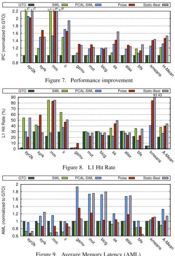
D. Performance

In Fig. 7, we demonstrate the performance ofPoise nor-malized to the baseline GTO scheduler for evaluation set workloads. We show that Poiseachieves a harmonic mean speedup of 46.6% (and up to 2.94×formm). In contrast, we observe a speedup of 31.5% with PCAL-SWL and 21.8% with SWL. Therefore, on average,Poiseoutperforms PCAL-SWL by 15.1% (up to 141.1% formm), and SWL by 24.8% (up to 49.4% forsyrk). We also observe that Static-Best achieves a harmonic mean speedup of 52.8%, surpassing PCAL-SWL by 21.3% on average (up to 182% formm). On the other hand, Static-Best surpassesPoiseby only 6.2% on average. This performance gap betweenPoiseand Static-Best can be attributed to the prediction errors in the regression model, and the slight search overhead to offset such errors at runtime. Notably, for some benchmarks, such assyrk,gsmv,mvtand

atax,Poiseeven surpasses the performance of Static-Best. We observe that these applications have monolithic kernels instead of several smaller kernels (as shown in Table IIIa). As a result,

Poiseis able to capture the dynamic phase changes within the

large monolithic kernels by performing predictions at regular intervals. However, these phases go undetected in Static-Best, where profiling is done offline at coarse kernel granularity.

Table IV

POISE PARAMETERS

Parameter Description Value

ω0,ω1,ω2 Performance scoring weights 1, 0.50, 0.25

Tperiod Inference periodicity 200,000 cycles

Twarmup Warmup duration 2,000 cycles

Tf eature Sampling duration for feature collection 10,000 cycles

Tsearch Sampling duration for local search 4,000 cycles

Imax Cut-off for instructions between global loads 49

εN Search stride forN 2

εp Search stride forp 4

Threshold speedup Speedup of a training kernel at best warp-tuple ≥1.5% Threshold cycles Execution cycles of a training kernel at baseline ≥10,000 cycles Threshold hit rate L1 hit rate for a training kernel atN=1,p=1 >0 %

We also note that for a few scenarios such assyr2kandbicg, SWL or PCAL-SWL perform better thanPoise. This happens when the global optimum lies within (or close to) the narrow reach of the SWL,i.e.,theN=pregion in the solution space. As both of these schemes use static SWL profiler, they get a head start by finding (or getting close to) the global optimum without incurring any runtime overheads.

E. L1 Cache Hit Rate

In Fig. 8, we compare theabsoluteL1 hit rate for different techniques. We observe thatPoiseachieves an average L1 hit rate of 40.1%, in contrast to 27.1% with PCAL-SWL, 37.7% with SWL, and 20.6% with baseline GTO. Therefore,Poise

outperforms PCAL-SWL by 13%, SWL by 2.4%, and GTO by 19.5% in cache performance. Notably, SWL comes close

toPoise in L1 hit rate, however, at the cost of significant

reduction in system performance. Lastly,Poisecomes close to the L1 hit rate of 43.6% achieved with Static-Best, indicating effective reduction of cache thrashing withPoise.

F. Average Memory Latency

To evaluate the performance of the shared memory system, we measure the average memory latencies (AML) incurred by L1 misses. In Fig. 9, we observe thatPoiseincreases the AML by only 1.1% over the baseline GTO scheduler. In contrast, PCAL-SWL increases the AML by 32.4%. This is because of the lower L1 hit rate in PCAL-SWL compared toPoise, which increases the memory traffic and aggravates congestion, thereby leading to high memory latencies. On the other hand, SWL decreases the AML by 10.7% but significantly underestimates the number of vital warps, indicated by the low speedup. Interestingly, AML with Static-Best increases by 14.1%, indicating that with optimal warp-tuples, SMs can tolerate a higher AML than baseline.

In summary, we observe thatPoiseprovides a good balance between TLP and cache performance (indicated by speedup and L1 hit rate), without under-utilizing or over-utilizing shared memory resources (indicated by AML).

G. Local Search Overhead

To analyze the search overhead, we measure the absolute displacement acrossNandpaxes between the predicted and subsequently searched warp-tuples in the {N, p} solution space. We also measure the net euclidean distance between the two points. In Fig. 10, we observe that on average, the final warp-tuple found after a local search is at an offset of 1.02 and 0.87 warps from the initial prediction inNandpaxis,

(11)

0.8 1 1.2 1.4 1.6 1.8 2 2.2

syr2k syrk mm ii gsmv mvt bicg ss atax bfs kmeans H-Mean

IPC (normalized to GTO)

GTO SWL PCAL-SWL Poise Static-Best

3.0 2.94 3.36 2.47 2.47

Figure 7. Performance improvement

0 10 20 30 40 50 60 70 80 90

syr2k syrk mm ii gsmv mvt bicg ss atax bfs kmeans A-Mean

L1 Hit Rate (%)

93.43

Figure 8. L1 Hit Rate

0.6 0.8 1 1.2 1.4 1.6 1.8 2

AML (normalized to GTO)

Figure 9. Average Memory Latency (AML)

respectively. This suggests that on average, local search in

Poiseconverges to an adjacentNandp(at an offset of around one warp each), thereby posing minimal overhead due to local search iterations. The overall euclidean distance between the predicted and locally searched warp-tuples is 1.59 on average. In the next subsection, we discuss the speedup observed with and without the local search inPoise(shown in Fig.11).

H. Sensitivity Study

Search stride:In Fig. 11, we vary the stride lengths forN

andp, represented by (εN,εp), which are used to perform a

local search around the predicted warp-tuples. We note that without performing any local search around the predicted warp-tuple,i.e., stride of (0, 0),Poiseachieves a harmonic mean speedup of 23% (up to 3.1×formm). Therefore, relying purely on predictions, with no local search,Poisestill achieves a higher speedup than SWL, while remaining only 8.5% short of PCAL-SWL performance, on average.

On increasing the search stride to (1, 1) and (2, 2), we observe the harmonic mean speedup of 43.6% and 45.7% respectively, which settles at 45% for a search stride of (4, 4). Therefore, we note that for most benchmarks, such assyr2k

and ii, increasing the stride length results in improvement at first, but it saturates or wears off with longer strides. On average, a stride of (2, 4) shows best speedup of 46.6%.

0 0.5 1 1.5 2 2.5 3 3.5 4

Absolute Displacement

N-axis p-axis Euclidean

Figure 10. Displacement between predicted and converged warp-tuples

0.6 0.8 1 1.2 1.4 1.6 1.8 2 2.2

IPC (normalized to baseline GTO)

(0, 0) (1, 1) (2, 2) (2, 4) (4, 4)

3.1 3.0 2.9 2.9 2.8

Figure 11. Sensitivity to search stride (εN,εp)

0.8 1 1.2 1.4 1.6 1.8 2 2.2

IPC (normalized to respective baseline)

Poise+16KB Poise+32KB Poise+64KB

5.3 5.7 5.0

Figure 12. Sensitivity to L1 cache size

L1 cache size:In this work,Poiseis trained on a GPU with 16 KB L1 cache, alongside a hash set-indexing function for L1. We now alter the architectural parameters of theevaluation platform, while using the previously trained regression model. For evaluation, we now employ a linear set-indexing function for L1 and vary the L1 cache size. In Fig. 12, we observe that with a 16 KB L1 cache,Poisemaintains a considerable harmonic mean speedup of 48%. Even on increasing the L1 cache size significantly by up to 4×(64 KB), we observe a harmonic mean speedup of 36.7%. Therefore,Poisecontinues to deliver performance improvements even with considerably larger caches. This also highlights the severity of the cache thrashing problem in GPUs. In summary, we observe thatPoise

remains effective even with changes to critical architectural features, such as L1 cache capacity and indexing, despite being trained on a different baseline.

Training features:We now examine the effect of removing a feature xi from the feature vector X, and retraining the

regression model withone lessattribute in the feature vector. The resultant speedup with such a model is shown in Fig. 13, normalized to the case whenallfeatures are used for training. In each of these cases, no local search is done around the initial predictions, so as to measure the change in the actual prediction accuracy. Also, we omitx1andx2from analysis as

(12)

0.6 0.7 0.8 0.9 1 1.1

IPC (normalized) all −x7 −x6 −x5 −x4 −x3 0.36 0.37 0.44 0.37

Figure 13. Sensitivity to removing a featurexifrom X

0 0.2 0.4 0.6 0.8 1

Energy consumption (normalized)

GTO Poise

Figure 14. Energy consumption

they are represented inx7and show a similar trend. We observe

that on removing a feature, the harmonic mean slowdown (compared to the case when all features are used for training) varies from 1.5% on removingx7to 21.7% on removingx6.

We note that highly memory-sensitive applications are most adversely impacted by the removal of a feature. Thus, best performance is shown when all features are used for training.

I. Hardware Costs

Area:Poiserequires seven 32-bit performance counters per SM to collect the parameters listed in Table II. Next,Poise

requires arithmetic resources to compute the link function. We note that computing the link function is not in the critical path and done rarely (once in every hundreds of thousands of cycles). In addition, prior work [12] has shown that in memory-sensitive applications, existing arithmetic units are idle for about 60% of the total execution time due to structural and data dependencies. Therefore, instead of introducing dedicated hardware to compute the link function, we time-multiplex the existing arithmetic units between SIMD instruction execution and link function computation. The link function is computed only during idle execution slots, and therefore it does not cause any performance penalty on original instruction throughput.

Poisealso requires one finite-state machine (FSM) per SM to

manage the state transition in HIE, requiring 7 states as per our implementation,i.e., two 3-bit state registers. Finally,Poise

adds one vital and cache-polluting bit for each warp in the warp scheduler queue, amounting to 96 bits per SM. In total,

Poiseposes a minimal storage overhead of 40.75 bytes per

SM and 1,304 bytes in total,i.e.,less than 0.01% of chip area, estimated using the existing parameters in GPUWattch [33]. In contrast, dynamic PCAL and CCWS implementations require CCWS-like hardware, includingvictim tag arrays, presenting greater storage overhead and lower performance. In summary,

Poiseis extremely lightweight in terms of storage.

0.8 1 1.2 1.4 1.6 1.8 2 2.2

GTO APCM Random-restart Poise 2.94

Figure 15. Performance with APCM and random-restart search policies

0 0.2 0.4 0.6 0.8 1 1.2

wc covar gramschm sradv2 hybridsort hotspot pathfinder H-Mean

GTO Poise P_best

Figure 16. Poiseon memory-insensitive applications

Energy: We now evaluate the energy consumption with

Poise. As shown in Fig. 14, we observe a reduction in overall energy consumption by 51.6% on average and up to 79.4% formm. This is partly because faster execution leads to lower leakage power dissipation. Additionally, better cache perfor-mance reduces off-chip memory accesses, thereby saving considerable data movement energy. Furthermore, the energy overhead due to the added hardware ofPoiseis negligible as it only requires few registers and an infrequent computation of the link function (once in hundreds of thousands of cycles).

J. Discussion

In this subsection, we discuss other topics related toPoise.

Cache bypassing:Cache bypassing schemes also aim to

improve memory system performance in GPUs. Therefore, we evaluatePoiseagainst APCM [28], state-of-the-art scheme to bypass and protect cache lines on the basis of instruction locality. APCM achieves this by filtering streaming accesses from high locality accesses. In Fig. 15, we observe thatPoise

outperforms APCM by 39.5% on average. This is because

Poisenot only improves memory system performance, but

also exercises greater control on the degree of multithreading, which is lacking in most bypassing schemes.

Stochastic search: Several stochastic search techniques have been proposed to overcome the problem of local optima in hill climbing [26], [44]. We evaluatePoiseagainst one such technique,i.e., random-restart with local search [37], [43]. In this scheme, we first choose arandomwarp-tuple as the starting point. This is followed by a local search (via gradient ascent) around the starting point, similar to the one used in

Poise. This process is repeated multiple times throughout

the execution with randomly selected starting points. The resultant performance is averaged over 20 executions of each benchmark to ensure statistically significant data. As shown in Fig. 15, we observe thatPoiseoutperforms random-restart

(13)

0 2 4 6 8 10 12 14 16 18 20 22 24 0 2 4 6 8 10 12 14 16 18 20 22 24 p (cache-polluting warps) N (vital warps) speedup slowdown MAX

(a) Static profile ofb f s

0 2 4 6 8 10 12 14 16 18 20 22 24 0 2 4 6 8 10 12 14 16 18 20 22 24 p (cache-polluting warps) N (vital warps) Warp samples Predicted Tuple Locally Searched Tuple

(b)Poiseexecution ofb f s

Figure 17. Observing correlation between static profile andPoise’s runtime execution for an unseen application.

search by 22.4% on average. This is because despite avoiding local optima, stochastic search techniques offer no guarantee of fast convergence to solution, often requiring high number of search iterations to converge due to a randomly selected starting point. By contrast,Poisebegins the search from a good initial starting point, which is expected to be close to the best warp-tuple (as shown in Fig. 10).

Compute-intensive applications:In Fig. 16, we

demon-strate the impact ofPoiseon compute-intensive applications that are insensitive to memory (Pbest <20%). We observe

a minor performance overhead of 1.6% on average, and a maximum of 3.5% forsradv2. Thus,Poiseis fairly benign to such applications. This is becausePoiseresorts to baseline behavior by employing maximum warps upon detecting compute-intensive behavior (as discussed in Section VI-A).

K. Case Study

We now present a case study for b f s, chosen from the evaluation set. Through this study, we qualitatively illustrate the accuracy of Poisein predicting good performing warp-tuples on a previously unseen benchmark. In Fig. 17a, we show the static performance profile forb f s. It indicates a general trend suggesting that the speedup improves with lower values ofNand p(green circles), with the best performing warp-tuple at (5, 5). It also indicates that there is an aversion to higher N and moderate-to-high p (red circles). Next, in Fig. 17b we show the different warp-tuples chosen by

Poiseat runtime, during the multiple prediction and local

search phases throughout the execution. The predicted warp-tuples are indicated by ‘+’ sign, whereas the warp-tuples generated after local search are indicated through the shaded coordinates. Therefore, we observe that most predictions are in the high performance zone, i.e., in close proximity of the best performing warp-tuple at (5, 5). Furthermore,Poise

successfully steers the system away from the low performance zones (red circles in Fig. 17a), thereby correctly detecting the general affinities in an entirely new benchmark.

VIII. RELATEDWORK

Cache Management: In addition to the state-of-the-art warp scheduling techniques discussed in Section III, several cache management schemes have been proposed to improve caching

efficiency. Improved cache performance helps in relieving the pressure on off-chip and on-chip memory bandwidth, which are critical resources in GPU [8], [9]. Liet al.[34] used reuse frequency and reuse distance to bypass the L1 cache for low locality accesses, using decoupled L1 data and tag arrays. Xie

et al.[50] proposed locality-driven cache bypassing at the

granularity of thread blocks. In contrast to bypassing schemes, we not only improve cache performance, but also alter the levels of multithreading. Furthermore, Chenet al.[7] proposed a coordinated cache bypassing and warp throttling scheme. However, similar to PCAL, they iteratively alter the number of warps by hill climbing to optimize NoC latencies. Therefore, it suffers from the same limitations as PCAL that were discussed previously in Section III-C. More recently, Lee and Wu [32] proposed an instruction-based scheme to bypass requests from low reuse memory instructions. Similarly, Kooet al. [28] proposed APCM, an instruction-based scheme to not only bypass, but also to protect cache lines using instruction locality characteristics (discussed in SectionVII-J). Furthermore, Jia

et al.[24] presented a taxonomy for memory access locality

and proposed a compile-time algorithm to selectively utilize the L1 caches for different locality types. Dublishet al.[11] proposed a cooperative caching mechanism to improve the aggregate caching efficiency by sharing reusable data among the L1 caches.

Machine Learning for Systems: There has been some prior

use of machine learning in computer architecture. Jim´enez and Lin [25] proposed a dynamic branch predictor based on the perceptron—the simplest neural network. ˙Ipeket al.[21] applied reinforcement learning to adaptively change DRAM scheduling decisions, instead of employing rigid policies. Liao

et al.[36] used machine learning to optimize memory prefetch

decisions in data centers by detecting the varying application needs. Machine learning has also been employed extensively to predict performance and power trends to avoid running full system simulations. ˙Ipeket al.[20] and Lee and Brooks [31] built design space models to predict the performance impact of architectural changes, saving simulation time. Similarly, Wu

et al. [49] used clustering algorithms and machine learning

in GPGPUs to estimate power and performance trends, using previously observed scaling behaviors.

In the realm of compilers, machine learning based tech-niques have proven to be extremely useful in finding good compiler optimizations. Stephensonet al. [46] used genetic algorithms to find optimizations by selecting and combining expressions of the cost functions based on their fitness to generate well performing code. Agakovet al.[2] used machine learning to correlate a new program with previously observed classes of programs. Using this prior knowledge, they propose a predictive model to focus the search on profitable areas of the solution space, speeding up iterative optimizations. Fursin

et al. [14] proposed MILEPOST GCC, a self-optimizing

compiler based on machine learning to optimize programs for evolving systems, such as reconfigurable processors.