Abstract—Steering control for path tracking in autonomous vehicles is well documented in the literature. Also, continuous direct yaw moment control, i.e., torque-vectoring, applied to human-driven electric vehicles with multiple motors is extensively researched. However, the combination of both controllers is not yet well understood. This paper analyzes the benefits of torque-vectoring in an autonomous electric vehicle, either by integrating the torque-vectoring system in the path tracking controller, or through its separate implementation alongside the steering controller for path tracking. A selection of path tracking controllers is compared in obstacle avoidance tests simulated with an experimentally validated vehicle dynamics model. A genetic optimization is used to select the controller parameters. Simulation results confirm that torque-vectoring is beneficial to autonomous vehicle response. The integrated controllers achieve the best performance if they are tuned for the specific tire-road friction condition. However, they can also cause unstable behavior when they operate in lower friction conditions without any re-tuning. On the other hand, separate torque-vectoring implementations provide consistently stable cornering response for a wide range of friction conditions. Controllers with preview formulations, or based on appropriate reference paths with respect to the middle line of the available lane, are beneficial to the path tracking performance.
Index Terms—Autonomous vehicle; electric vehicle; path tracking control; torque-vectoring control; optimization; vehicle dynamics
I. INTRODUCTION
Autonomous vehicles require path tracking controllers (PTCs) that ensure safe behavior even in extreme maneuvers. Most of the path tracking (PT) studies (see the survey in [1]) focus on steering actuation. A large body of literature on steering control for PT was initially developed with the purpose of driver modeling [2]–[7]. In fact, the human driver can be seen as an advanced adaptive PTC actuating the steering wheel. Hence, driver models can perform as automated PTCs as well, provided that human physiology limitations are not considered in their formulations. In recent years the research focus has shifted from driver modeling to autonomous driving applications [8]–[14]. In this respect, [15] compares the
performance of multiple steering based PTCs for autonomous vehicles.
Another topic extensively discussed in the literature is torque-vectoring (TV), i.e., the control of the traction and braking torque of each wheel to generate a direct yaw moment. TV controllers (TVCs) are easily implementable in electric vehicles (EVs) with individual wheel motors, since these solutions allow precise wheel torque controllability, usually with higher bandwidth than the conventional friction brakes and internal combustion engine drivetrains. In human driven EVs, TVCs can enhance the cornering response, e.g., by shaping the understeer characteristic, increasing agility and ensuring stability in extreme transients [16]-[23]. TVCs are usually implemented as yaw rate feedforward / feedback controllers, with the option of sideslip contributions.
In autonomous EVs the TVC can be an independent controller receiving the automated steering angle as an input from the PTC, and thus generating a reference yaw rate that has to be tracked by the TVC itself [24]. Alternatively, steering actuation and TV can be merged to become the outputs of an integrated PTC, without the need for a reference yaw rate to be tracked by the TVC. In this respect, [25]-[31] propose PTCs with integrated steering and direct yaw moment control. [32] is a comparative study between model predictive control (MPC) and a linear quadratic regulator (LQR) for integrated PTC, tuned through a trial-and-error process. However, it is yet unknown if the integrated PTCs present benefits compared to the multi-layer control structures consisting of independent steering controllers for PT (top layer) and TVCs for yaw rate and sideslip tracking (bottom layer).
This study addresses this knowledge gap by assessing the two architectural control system designs during obstacle avoidance maneuvers simulated with an experimentally validated vehicle simulation model. The points of novelty are:
The integration of TV with multiple steering based PTCs from the literature. Both single-point PTCs without preview and multiple-point preview PTCs are used.
The stochastic optimization of the PTC parameters to achieve a fair comparison among the control structures.
Comparison of Path Tracking and
Torque-Vectoring Controllers for Autonomous Electric
Vehicles
Christoforos Chatzikomis1, Aldo Sorniotti1,*,
Member
,
IEEE
,
Patrick Gruber1, Mattia Zanchetta1, Dan Willans2, Bryn Balcombe21University of Surrey, United Kingdom 2Roborace, United Kingdom
The objective comparison of the performance of the separate and integrated steering and yaw moment controllers.
II. THE CASE STUDY AUTONOMOUS ELECTRIC VEHICLE
A. EV hardware
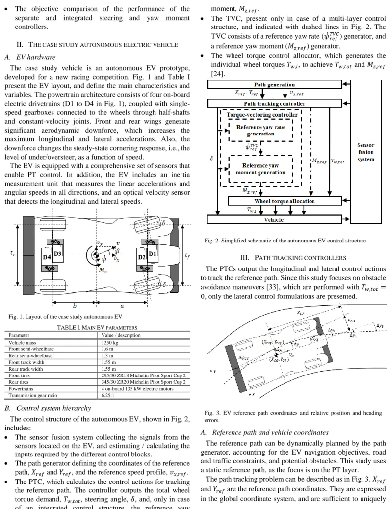
The case study vehicle is an autonomous EV prototype, developed for a new racing competition. Fig. 1 and Table I present the EV layout, and define the main characteristics and variables. The powertrain architecture consists of four on-board electric drivetrains (D1 to D4 in Fig. 1), coupled with single-speed gearboxes connected to the wheels through half-shafts and constant-velocity joints. Front and rear wings generate significant aerodynamic downforce, which increases the maximum longitudinal and lateral accelerations. Also, the downforce changes the steady-state cornering response, i.e., the level of under/oversteer, as a function of speed.
The EV is equipped with a comprehensive set of sensors that enable PT control. In addition, the EV includes an inertia measurement unit that measures the linear accelerations and angular speeds in all directions, and an optical velocity sensor that detects the longitudinal and lateral speeds.
Fig. 1. Layout of the case study autonomous EV TABLEI.MAIN EV PARAMETERS
Parameter Value / description
Vehicle mass 1250 kg
Front semi-wheelbase 1.6 m
Rear semi-wheelbase 1.3 m
Front track width 1.55 m
Rear track width 1.55 m
Front tires 295/30 ZR18 Michelin Pilot Sport Cup 2
Rear tires 345/30 ZR20 Michelin Pilot Sport Cup 2
Powertrains 4 on-board 135 kW electric motors
Transmission gear ratio 6.25:1
B. Control system hierarchy
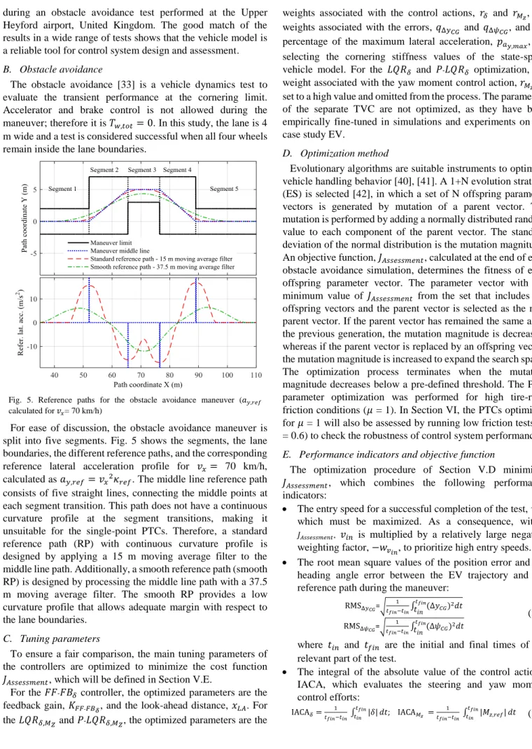
The control structure of the autonomous EV, shown in Fig. 2, includes:
The sensor fusion system collecting the signals from the sensors located on the EV, and estimating / calculating the inputs required by the different control blocks.
The path generator defining the coordinates of the reference path, 𝑋𝑟𝑒𝑓 and 𝑌𝑟𝑒𝑓, and the reference speed profile, 𝑣𝑥,𝑟𝑒𝑓.
The PTC, which calculates the control actions for tracking the reference path. The controller outputs the total wheel torque demand, 𝑇𝑤,𝑡𝑜𝑡, steering angle, 𝛿, and, only in case of an integrated control structure, the reference yaw
moment, 𝑀𝑧,𝑟𝑒𝑓.
The TVC, present only in case of a multi-layer control structure, and indicated with dashed lines in Fig. 2. The TVC consists of a reference yaw rate (𝜓̇𝑟𝑒𝑓𝑇𝑉𝐶) generator, and a reference yaw moment (𝑀𝑧,𝑟𝑒𝑓) generator.
The wheel torque control allocator, which generates the individual wheel torques 𝑇𝑤,𝑖, to achieve 𝑇𝑤,𝑡𝑜𝑡 and 𝑀𝑧,𝑟𝑒𝑓 [24].
Fig. 2. Simplified schematic of the autonomous EV control structure
III. PATH TRACKING CONTROLLERS
The PTCs output the longitudinal and lateral control actions to track the reference path. Since this study focuses on obstacle avoidance maneuvers [33], which are performed with 𝑇𝑤,𝑡𝑜𝑡= 0, only the lateral control formulations are presented.
Fig. 3. EV reference path coordinates and relative position and heading errors
A. Reference path and vehicle coordinates
The reference path can be dynamically planned by the path generator, accounting for the EV navigation objectives, road and traffic constraints, and potential obstacles. This study uses a static reference path, as the focus is on the PT layer.
The path tracking problem can be described as in Fig. 3. 𝑋𝑟𝑒𝑓 and 𝑌𝑟𝑒𝑓 are the reference path coordinates. They are expressed
define the reference path. In the remainder the capital letters 𝑋 and 𝑌 will be used to express coordinates in the global reference system, while 𝑥 and 𝑦 will be adopted for coordinates in the vehicle reference system. The reference heading (yaw) angle, 𝜓𝑟𝑒𝑓, and the reference curvature, 𝜅𝑟𝑒𝑓, are derived from the
reference coordinates and used by the PTCs.
Since the EV deviates from the reference path, the actual distance traveled by the EV, 𝑠, is not equal to the length of the reference path. By assuming small sideslip angles, the distance travelled along the reference path during the maneuver is given by [7]:
𝑠 = ∫ 𝑣𝑥cos(∆𝜓𝐶𝐺) − 𝑣𝑦𝑠𝑖𝑛(∆𝜓𝐶𝐺)
1 − 𝜅𝑟𝑒𝑓[(𝑌𝐶𝐺− 𝑌𝑟𝑒𝑓) cos 𝜓𝑟𝑒𝑓− (𝑋𝐶𝐺− 𝑋𝑟𝑒𝑓) 𝑠𝑖𝑛𝜓𝑟𝑒𝑓]𝑑𝑡 (1)
where 𝑣𝑥 and 𝑣𝑦 are the longitudinal and lateral EV speeds, and 𝑋𝐶𝐺 and 𝑌𝐶𝐺 are the coordinates of the vehicle center of gravity
(CG). The lateral position error, Δ𝑦𝐶𝐺, and heading angle error,
∆𝜓𝐶𝐺, of the EV CG in relation to the reference path are defined
as in Fig. 3:
Δ𝑦𝐶𝐺= (𝑌𝐶𝐺− 𝑌𝑟𝑒𝑓) cos 𝜓𝑟𝑒𝑓− (𝑋𝐶𝐺− 𝑋𝑟𝑒𝑓) 𝑠𝑖𝑛𝜓𝑟𝑒𝑓
Δ𝜓𝐶𝐺= 𝜓 − 𝜓𝑟𝑒𝑓
(2) where 𝜓 is the EV heading angle.
B. 𝐹𝐹-𝐹𝐵𝛿: feedforward-feedback steering controller
The first PTC of this study is the feedforward-feedback controller, 𝐹𝐹-𝐹𝐵𝛿, recently presented in [34], which has been
experimentally demonstrated at the limit of handling. The steering angle control law consists of feedforward and feedback contributions:
𝛿 = 𝛿𝐹𝐹+ 𝛿𝐹𝐵 (3)
The feedforward term, 𝛿𝐹𝐹, is based on the steady-state
cornering response of the single-track vehicle model:
𝛿𝐹𝐹= 𝑙𝜅𝑟𝑒𝑓− (𝛼𝐹𝐹𝐹− 𝛼𝑅𝐹𝐹) (4)
where 𝑙 is the wheelbase. The term 𝑙𝜅𝑟𝑒𝑓 is the kinematic steering angle corresponding to the reference path curvature. 𝛼𝐹𝐹𝐹 and 𝛼𝑅𝐹𝐹 are the lumped slip angles of the front and rear
tires. 𝛼𝐹𝐹𝐹 and 𝛼𝑅𝐹𝐹 are calculated from an inverse tire model, taking into account the vertical load transfers, so that they generate the respective feedforward lateral tire forces on the front and rear axles, 𝐹𝑦,𝐹𝐹𝐹 and 𝐹𝑦,𝑅𝐹𝐹. These are determined under the assumption that the vehicle achieves the reference lateral acceleration, 𝑣𝑥2𝜅𝑟𝑒𝑓, calculated for steady-state cornering.
Based on the lateral force and yaw moment balance equations in steady-state conditions, 𝐹𝑦,𝐹𝐹𝐹 and 𝐹𝑦,𝑅𝐹𝐹 are:
{𝐹𝑦,𝐹 𝐹𝐹=𝑚𝑏 𝑙 𝑣𝑥2𝜅𝑟𝑒𝑓− 𝑀𝑧,𝑟𝑒𝑓 𝑙 𝐹𝑦,𝑅𝐹𝐹=𝑚𝑎 𝑙 𝑣𝑥2𝜅𝑟𝑒𝑓+ 𝑀𝑧,𝑟𝑒𝑓 𝑙 (5) where 𝑚 is the vehicle mass, and 𝑎 and 𝑏 are the front and rear semi-wheelbases.
The feedback term, 𝛿𝐹𝐵, is designed to control the corrected
look-ahead error, 𝑒𝐿𝐴,𝑐𝑜𝑟𝑟, and is defined as:
𝛿𝐹𝐵= −𝐾𝑃𝑇𝐶1𝑒𝐿𝐴,𝑐𝑜𝑟𝑟= −𝐾𝑃𝑇𝐶1[Δ𝑦𝐶𝐺+ 𝑥𝐿𝐴(Δ𝜓𝐶𝐺+ 𝛽𝑠𝑠)] (6)
𝛽𝑠𝑠= 𝛼𝑅𝐹𝐹+ 𝑏𝜅𝑟𝑒𝑓 (7)
where 𝐾𝑃𝑇𝐶1 is the proportional (P) gain. The term 𝑒𝐿𝐴= Δ𝑦𝐶𝐺+
𝑥𝐿𝐴Δ𝜓𝐶𝐺 is the look-ahead error, i.e., the tracking error projected
at a distance 𝑥𝐿𝐴 in front of the vehicle, as shown in Fig. 3. For the lateral deviation to be zero, the vehicle sideslip angle 𝛽 is incorporated in the feedback law, which is then based on 𝑒𝐿𝐴,𝑐𝑜𝑟𝑟. To avoid relying on the real-time measurement or
estimation of 𝛽, as suggested in [34] eq. (6) uses 𝛽𝑠𝑠, which is
the steady-state value of 𝛽 corresponding to the reference curvature, according to eq. (7).
C. 𝐿𝑄𝑅𝛿,𝑀𝑍: linear quadratic regulator without preview (integrated controller)
The second controller is based on the LQR formulation for steering control in [15], which is extended to include the reference yaw moment.
The state-space formulation of the single-track vehicle model for path tracking control is:
[ Δ𝑦̇𝐶𝐺 Δ𝑦̈𝐶𝐺 ∆𝜓̇𝐶𝐺 Δ𝜓̈𝐶𝐺] = [ 0 1 0 −𝐶𝑓+ 𝐶𝑟 𝑚𝑣𝑥 0 0 𝐶𝑓+ 𝐶𝑟 𝑚 𝑏𝐶𝑟− 𝑎𝐶𝑓 𝑚𝑣𝑥 0 0 0 𝑏𝐶𝑟− 𝑎𝐶𝑓 𝐼𝑧𝑣𝑥 0 1 𝑎𝐶𝑓− 𝑏𝐶𝑟 𝐼𝑧 − 𝑎2𝐶 𝑓+ 𝑏2𝐶𝑟 𝐼𝑧𝑣𝑥 ] [ Δ𝑦𝐶𝐺 Δ𝑦̇𝐶𝐺 Δ𝜓𝐶𝐺 ∆𝜓̇𝐶𝐺] + [ 0 0 𝐶𝑓 𝑚 0 0 0 𝑎𝐶𝑓 𝐼𝑧 1 𝐼𝑧] [𝑀𝛿 𝑧] + [ 0 𝑏𝐶𝑟− 𝑎𝐶𝑓 𝑚𝑣𝑥 − 𝑣𝑥 0 𝑎2𝐶 𝑓+ 𝑏2𝐶𝑟 𝐼𝑧𝑣𝑥 ] 𝜓̇𝑟𝑒𝑓+ [ 0 0 0 −1 ] 𝜓̈𝑟𝑒𝑓 (8)
where 𝐼𝑧 is the yaw mass moment of inertia. 𝐶𝑓 and 𝐶𝑟 are the cornering stiffness values of the front and rear axles. In this study, these are selected at a specific percentage, 𝑝𝑎𝑦,𝑚𝑎𝑥, of the
maximum 𝑎𝑦 achieved in steady-state conditions, according to
the approach in [35]. In eq. (8) the state variables of the single-track vehicle model, i.e., 𝑣𝑦 and 𝜓̇, are converted into the error
state variables with respect to the reference path: 𝑣𝑦= Δ𝑦̇𝐶𝐺− 𝑣𝑥 ∆𝜓𝐶𝐺
𝜓̇ = Δ𝜓̇𝐶𝐺+ 𝜓̇𝑟𝑒𝑓
(9) Eq. (8) can be re-written in the following matrix form:
𝑿̇ = 𝑨𝑿 + 𝑩𝟏𝑼 + 𝑩𝟐𝜓̇𝑟𝑒𝑓+ 𝑩𝟑𝜓̈𝑟𝑒𝑓 where 𝑿 = [ Δ𝑦𝐶𝐺 Δ𝑦̇𝐶𝐺 Δ𝜓𝐶𝐺 ∆𝜓̇𝐶𝐺] and𝑈 = [𝑀𝛿 𝑧] (10) The terms associated with the reference path yaw rate and acceleration, 𝑩𝟐𝜓̇𝑟𝑒𝑓 and 𝑩𝟑𝜓̈𝑟𝑒𝑓, are external disturbances. The state-space formulation is discretized as:
𝑿(𝑘 + 1) = 𝑨𝒌𝑿(𝑘) + 𝑩𝟏,𝒌𝑼(𝑘) (11)
The feedback control gains minimize the cost function 𝐽𝑃𝑇𝐶2:
𝐽𝑃𝑇𝐶2= ∑ 𝑿(𝑘)𝑇𝑸𝑿(𝑘) + 𝑼(𝑘)𝑇𝑹𝑼(𝑘) ∞ 𝑘=1 𝑸 = [ 𝑞Δ𝑦𝐶𝐺 0 0 0 0 0 0 0 0 0 𝑞Δ𝜓𝐶𝐺 0 0 0 0 0 ], 𝑹 = [𝑟0 𝑟𝛿 0 𝑀𝑧 ] (12)
The weighting factors 𝑞Δ𝑦𝐶𝐺 and 𝑞Δ𝜓𝐶𝐺 define the relative importance of the lateral displacement and heading angle errors, while 𝑟𝛿 and 𝑟𝑀𝑧 define the relative significance of the steering
calculated with the Riccati equation [36], are scheduled with vehicle speed, 𝑣𝑥, which is a parameter in eq. (11). The feedback control law is expressed as a function of the lateral position and heading angle errors, and their time derivatives:
[𝛿𝐹𝐵 𝑀𝑧,𝐹𝐵] = 𝑲(𝑣𝑥) [ Δ𝑦𝐶𝐺 Δ𝑦̇𝐶𝐺 Δ𝜓𝐶𝐺 ∆𝜓̇𝐶𝐺] 𝑲(𝑣𝑥) = [ 𝑘𝛿,Δ𝑦𝐶𝐺 𝑘𝛿,Δ𝑦̇𝐶𝐺 𝑘𝑀𝑧,Δ𝑦𝐶𝐺 𝑘𝑀𝑧,Δ𝑦̇𝐶𝐺 𝑘𝛿,Δ𝜓𝐶𝐺 𝑘𝛿,∆𝜓̇𝐶𝐺 𝑘𝑀𝑧,Δ𝜓𝐶𝐺 𝑘𝑀𝑧,∆𝜓̇𝐶𝐺] (13)
The 𝐿𝑄𝑅𝛿,𝑀𝑍 can be combined with a feedforward contribution in terms of steering angle and yaw moment, thus giving origin to the 𝐿𝑄𝑅𝛿,𝑀𝑍,𝐹𝐹. The same formulation as in eq.
(4) is used for the feedforward steering contribution, 𝛿𝐹𝐹. The
reference yaw acceleration, 𝜓̈𝑟𝑒𝑓, corresponding to the time
derivative of the curvature of the reference path, is adopted for the feedforward yaw moment contribution, 𝑀𝑧,𝐹𝐹:
𝑀𝑧,𝐹𝐹= 𝑐𝑀𝑧,𝐹𝐹𝜓̈𝑟𝑒𝑓𝐼𝑧
𝜓̈𝑟𝑒𝑓= 𝑣𝑥𝜅̇𝑟𝑒𝑓
(14) As 𝜓̈𝑟𝑒𝑓has to be generated by the total yaw moment, caused by
both the longitudinal and lateral tire forces, the scaling factor
0 ≤ 𝑐𝑀𝑧,𝐹𝐹≤ 1 accounts for the fact that 𝑀𝑧,𝐹𝐹 is the
feedforward yaw moment generated only by the longitudinal tire forces.
D. 𝑃-𝐿𝑄𝑅𝛿,𝑀𝑍: linear quadratic regulator with preview
(integrated controller)
The third controller includes a preview model according to the formulation in [37], which is limited to the case of steering control. In this study the algorithm is extended to include the yaw moment contribution. Under the hypothesis of small heading angles, the single-track vehicle model equations are reformulated in the global coordinate system as:
[ 𝑌𝐶𝐺̇ 𝑌̈𝐶𝐺 𝜓̇ 𝜓̈ ] = [ 0 1 0 −𝐶𝑓+ 𝐶𝑟 𝑚𝑣𝑥 0 0 𝐶𝑓+ 𝐶𝑟 𝑚 𝑏𝐶𝑟− 𝑎𝐶𝑓 𝑚𝑣𝑥 0 0 0 𝑏𝐶𝑟− 𝑎𝐶𝑓 𝐼𝑧𝑣𝑥 0 1 𝑎𝐶𝑓− 𝑏𝐶𝑟 𝐼𝑧 − 𝑎2𝐶 𝑓+ 𝑏2𝐶𝑟 𝐼𝑧𝑣𝑥 ] [ 𝑌𝐶𝐺 𝑌̇𝐶𝐺 𝜓 𝜓̇ ] + [ 0 0 𝐶𝑓 𝑚 0 0 0 𝑎𝐶𝑓 𝐼𝑧 1 𝐼𝑧] [𝑀𝛿 𝑧] (15) 𝑿̇𝒗= 𝑨𝒗𝑿𝒗+ 𝑩𝒗𝑼 𝑿𝒗= [ 𝑌𝐶𝐺 𝑌̇𝐶𝐺 𝜓 𝜓̇ ] , 𝑼 = [𝑀𝛿 𝑧] (16)
and then they can be discretized as:
𝑿𝒗(𝑘 + 1) = 𝑨𝒗,𝒌𝑿𝒗(𝑘) + 𝑩𝒗,𝒌𝑼(𝑘) (17)
The road preview profile is defined as a shift register, where 𝒚𝒓(𝑘) is the vector of lateral deviations from the reference path
along a preview axis in front of the vehicle, and Δ𝑦𝑛𝑝 (= ∆𝑦5 in Fig. 3) is the final input to the road system, i.e., the new lateral deviation value.
𝒚𝒓(𝑘 + 1) = 𝑨𝒓,𝒌𝒚𝒓(𝑘) + 𝑩𝒓,𝒌Δ𝑦𝑛𝑝 (18) 𝑨𝒓𝒌= [ 0 1 0 0 0 01 0 ⋯ 0⋯ 0 ⋮ ⋮ ⋮ ⋮ ⋮ ⋱⋮ ⋱ ⋱ ⋮⋱ 0 0 0 0 0 0 ⋯0 ⋯ ⋯ 1⋯ 0] , 𝑩𝒓𝒌= [ 0 0 0 ⋮ 1]
Eq. (17) and eq. (18) are combined into the state-space formulation of the preview LQR problem:
[𝑿𝒗(𝑘 + 1) 𝒚𝒓(𝑘 + 1)] = [ 𝑨𝒗,𝒌 0 0 𝑨𝒓,𝒌] [ 𝑿𝒗(𝑘) 𝒚𝒓(𝑘)] + [ 𝑩𝒗,𝒌 0 ] 𝑼(𝑘) + [ 0 𝑩𝒓𝒌 ] Δ𝑦𝑛𝑝 (19) The state vector is defined as 𝒁 = [𝑿𝒗 𝒚𝒓]𝑇, and the term [𝑩0
𝒓𝒌] Δ𝑦𝑛𝑝is consideredan external disturbance, such that the equations are expressed in the standard LQR form.
The LQR cost function is:
𝐽𝑃𝑇𝐶3= ∑ 𝒁(𝑘)𝑇𝑸𝒁(𝑘) + 𝑼(𝑘)𝑇𝑹𝑼(𝑘) ∞ 𝑘=1 where 𝑹 = [𝑟0 𝑟𝛿 0 𝑀𝑧 ], 𝑸 = 𝑪𝑇[𝑞Δ𝑦𝐶𝐺 0 0 𝑞Δ𝜓𝐶𝐺 ] 𝑪 and 𝑪 = [ 1 0 0 0 −1 0 0 … 0 0 0 1 0 1 𝑣𝑥𝑇𝑠 − 1 𝑣𝑥𝑇𝑠 0 … 0] (20)
𝑇𝑠 is the controller sample time. The weight matrix 𝑪 defines
the link between the vehicle and road preview. The first row of 𝑪 is formulated to minimize the sum of the squares of the lateral displacement error, Δ𝑦𝐶𝐺, and the second row to minimize the
square of the heading error at the center of gravity, calculated as (𝜓𝐶𝐺−Δ𝑦1−Δ𝑦𝐶𝐺
𝑣𝑥𝑇𝑠 ) 2
. After a re-arrangement in local vehicle coordinates (see [37]), the control law is given in eq. (21), with the preview and state feedback gains scheduled with 𝑣𝑥:
[𝑀𝛿 𝑧,𝐹𝐵] = 𝑲𝒑𝒓𝒗(𝑣𝑥) [ 𝑣𝑦 𝜓̇ Δ𝑦𝐶𝐺 Δ𝑦1 ⋮ Δ𝑦𝑛𝑝] 𝑲𝒑𝒓𝒗(𝑣𝑥) = [ 𝑘𝛿,𝑦̇𝐶𝐺 𝑘𝑀𝑧,𝑦̇𝐶𝐺 𝑘𝛿,𝜓̇𝐶𝐺 𝑘𝛿,Δ𝑦𝐶𝐺 𝑘𝛿,Δ𝑦1 … 𝑘𝛿,Δ𝑦𝑛𝑝 𝑘𝑀𝑧,𝜓̇𝐶𝐺 𝑘𝑀𝑧,Δ𝑦𝐶𝐺 𝑘𝑀𝑧,Δ𝑦1 … 𝑘𝑀𝑧,Δ𝑦𝑛𝑝 ] (21)
E. 𝐿𝑄𝑅𝛿 and 𝑃-𝐿𝑄𝑅𝛿: linear quadratic regulators for steering
control
In this study the LQRs of Sections III.C and III.D are also considered in their original formulations, reported in [15] and [37], excluding the direct yaw moment. These, respectively indicated as 𝐿𝑄𝑅𝛿 and 𝑃-𝐿𝑄𝑅𝛿, can either operate on their own,
or can be part of a multi-layer structure, including the TVC presented in Section IV.
IV. TORQUE-VECTORING CONTROLLER (TVC) A separate TVC was developed to assess the effectiveness of the multi-layer PTC+TVC structures. The details of the TVC design and functionality are presented in [24]. The TVC includes a reference yaw rate generator and a reference yaw moment generator, and together with the PTCs of Section III uses a wheel torque control allocation algorithm.
A. Reference yaw rate generator
The steady-state value of the TVC reference yaw rate, 𝜓̇𝑟𝑒𝑓,𝑆𝑆𝑇𝑉𝐶 , is the weighted average of two yaw rate values (see [24], [38]
and [39]), 𝜓̇𝑟𝑒𝑓,𝐻𝑇𝑉𝐶 and 𝜓̇𝑟𝑒𝑓,𝑆𝑇𝑉𝐶 :
𝜓̇𝑟𝑒𝑓,𝑆𝑆𝑇𝑉𝐶 = 𝜓̇
𝑟𝑒𝑓,𝐻𝑇𝑉𝐶 𝑤𝛽+ 𝜓̇𝑟𝑒𝑓,𝑆𝑇𝑉𝐶 (1 − 𝑤𝛽) (22)
The handling yaw rate, 𝜓̇𝑟𝑒𝑓,𝐻𝑇𝑉𝐶 , corresponds to the reference steady-state EV cornering behavior in nominal high tire-road friction conditions. 𝜓̇𝑟𝑒𝑓,𝐻𝑇𝑉𝐶 is defined in a look-up table, which is a function of steering angle, vehicle speed and longitudinal acceleration. 𝜓̇𝑟𝑒𝑓,𝐻𝑇𝑉𝐶 is designed to shape the vehicle understeer characteristics, which can be rather different from those of the uncontrolled vehicle with identical wheel torques on the left- and right-hand sides [16]. The stability yaw rate, 𝜓̇𝑟𝑒𝑓,𝑆𝑇𝑉𝐶 , is a conservative yaw rate that is compatible with the actual tire-road friction conditions, i.e., it is based on the measured lateral acceleration (𝑎𝑦) value.
To determine if the EV operates in different conditions from the nominal ones, the sideslip angle of the rear axle, 𝛽𝑟, is considered [38]:
𝛽𝑟= 𝛽 −
𝑏𝑟
𝑣𝑥 (23)
Large values of |𝛽𝑟| indicate saturation of the rear lateral tire forces, which can lead to oversteer and, ultimately, vehicle spinning. The weighting factor 𝑤𝛽 determines the significance
of the 𝜓̇𝑟𝑒𝑓,𝐻𝑇𝑉𝐶 and 𝜓̇𝑟𝑒𝑓,𝑆𝑇𝑉𝐶 contributions of 𝜓̇𝑟𝑒𝑓,𝑆𝑆𝑇𝑉𝐶 . When |𝛽𝑟| is
lower than a first threshold (𝛽𝑟,𝑡ℎ,1), 𝜓̇𝑟𝑒𝑓,𝑆𝑆𝑇𝑉𝐶 is equal to the
handling yaw rate, while when |𝛽𝑟| is higher than a second threshold (𝛽𝑟,𝑡ℎ,2), 𝜓̇𝑟𝑒𝑓,𝑆𝑆𝑇𝑉𝐶 is equal to the stability yaw rate, with
a smooth transition between the two extreme cases: 𝑤𝛽= { 1 𝑖𝑓 |𝛽𝑟| < 𝛽𝑟,𝑡ℎ,1 𝛽𝑟,𝑡ℎ,2− |𝛽𝑟| 𝛽𝑟,𝑡ℎ,2− 𝛽𝑟,𝑡ℎ,1 𝑖𝑓 𝛽𝑟,𝑡ℎ,1≤ |𝛽𝑟| ≤ 𝛽𝑟,𝑡ℎ,2 0 𝑖𝑓 |𝛽𝑟| > 𝛽𝑟,𝑡ℎ,2 (24) In practice, when the EV operates in low friction or extreme transient conditions, 𝛽𝑟 is limited between the two thresholds
through the adjustment of 𝜓̇𝑟𝑒𝑓,𝑆𝑆𝑇𝑉𝐶 . Different sets of thresholds can be defined. In particular, the following two settings are used in this study:
High sideslip setting: 𝛽𝑟,𝑡ℎ,1 = 4.5 deg, 𝛽𝑟,𝑡ℎ,2 = 9 deg,
which is adopted in high tire-road friction conditions (tests with 𝜇 = 1).
Low sideslip setting: 𝛽𝑟,𝑡ℎ,1 = 2 deg, 𝛽𝑟,𝑡ℎ,2 = 4 deg, which
is adopted in low friction conditions (tests with 𝜇 = 0.6). Since the case study EV is for racing applications, the tire-road friction level can be considered approximately known a-priori depending on the condition of the tarmac (e.g., dry or wet), and the switching between the two settings can be imposed without
a tire-road friction coefficient estimator. In any case, the simulations and experiments on the case study EV demonstrated that both tunings provide stable and predictable behavior for the whole range of 𝜇 values.
A first order transfer function generates the reference yaw rate, 𝜓̇𝑟𝑒𝑓𝑇𝑉𝐶, starting from 𝜓̇𝑟𝑒𝑓,𝑆𝑆𝑇𝑉𝐶 . Note that the resulting 𝜓̇𝑟𝑒𝑓𝑇𝑉𝐶, mainly based on 𝛿, differs from the reference yaw rate of the PTCs in Section III, which is purely based on the reference path.
B. Reference yaw moment generator
The reference yaw moment generator is based on a non-linear feedforward contribution and a feedback contribution. The feedforward contribution is computed off-line through a quasi-static model, to achieve 𝜓̇𝑟𝑒𝑓,𝑆𝑆𝑇𝑉𝐶 when the EV operates in high tire-road friction conditions with quasi-static steering inputs, and is defined as a look-up table, which is a function of steering angle, vehicle speed and longitudinal acceleration. Similarly to 𝜓̇𝑟𝑒𝑓,𝑆𝑆𝑇𝑉𝐶 , the feedforward yaw moment contribution is corrected
to account for low tire-road friction conditions and transient behavior, based on |𝛽𝑟|. The feedback contribution is a
proportional integral (PI) controller with anti-windup and gain scheduling with 𝑣𝑥. The reference yaw moment is saturated
through the continuous estimation of the EV operational limits, based on the drivetrain torque limits and the estimated individual tire friction limits.
C. Wheel torque control allocator
A wheel torque control allocation scheme determines the individual reference wheel torques. Firstly, the control allocator calculates the total wheel torque required on the left- and right-hand sides of the EV to generate the total reference wheel torque and reference yaw moment. Within each side the torque demand is then distributed proportionally to the estimated vertical tire loads, subject to individual wheel and drivetrain torque limitations. The same wheel torque control allocator is used by the separate TVC and the integrated PTCs, as shown in Fig. 2.
V. SIMULATION AND CONTROL SYSTEM OPTIMIZATION FRAMEWORK
A. Experimentally validated simulation model
A non-linear vehicle dynamics simulation model was implemented in Matlab/Simulink and validated against experimental measurements on the case study EV, with and without the TVC of Section IV. Fig. 4 shows an example of simulation and experimental results for the case study EV
during an obstacle avoidance test performed at the Upper Heyford airport, United Kingdom. The good match of the results in a wide range of tests shows that the vehicle model is a reliable tool for control system design and assessment.
B. Obstacle avoidance
The obstacle avoidance [33] is a vehicle dynamics test to evaluate the transient performance at the cornering limit. Accelerator and brake control is not allowed during the maneuver; therefore it is 𝑇𝑤,𝑡𝑜𝑡= 0. In this study, the lane is 4
m wide and a test is considered successful when all four wheels remain inside the lane boundaries.
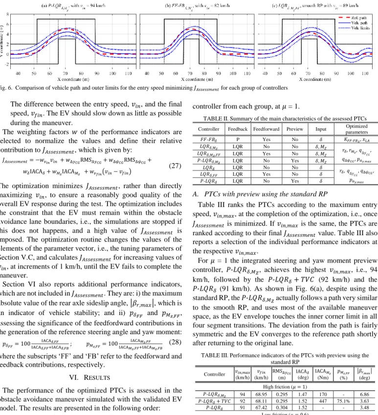
For ease of discussion, the obstacle avoidance maneuver is split into five segments. Fig. 5 shows the segments, the lane boundaries, the different reference paths, and the corresponding reference lateral acceleration profile for 𝑣𝑥= 70 km/h,
calculated as 𝑎𝑦,𝑟𝑒𝑓= 𝑣𝑥2𝜅𝑟𝑒𝑓. The middle line reference path consists of five straight lines, connecting the middle points at each segment transition. This path does not have a continuous curvature profile at the segment transitions, making it unsuitable for the single-point PTCs. Therefore, a standard reference path (RP) with continuous curvature profile is designed by applying a 15 m moving average filter to the middle line path. Additionally, a smooth reference path (smooth RP) is designed by processing the middle line path with a 37.5 m moving average filter. The smooth RP provides a low curvature profile that allows adequate margin with respect to the lane boundaries.
C. Tuning parameters
To ensure a fair comparison, the main tuning parameters of the controllers are optimized to minimize the cost function 𝐽𝐴𝑠𝑠𝑒𝑠𝑠𝑚𝑒𝑛𝑡, which will be defined in Section V.E.
For the 𝐹𝐹-𝐹𝐵𝛿 controller, the optimized parameters are the feedback gain, 𝐾𝐹𝐹-𝐹𝐵𝛿, and the look-ahead distance, 𝑥𝐿𝐴. For the 𝐿𝑄𝑅𝛿,𝑀𝑍 and 𝑃-𝐿𝑄𝑅𝛿,𝑀𝑍, the optimized parameters are the
weights associated with the control actions, 𝑟𝛿 and 𝑟𝑀𝑧, the weights associated with the errors, 𝑞Δ𝑦𝐶𝐺 and 𝑞Δ𝜓𝐶𝐺, and the
percentage of the maximum lateral acceleration, 𝑝𝑎𝑦,𝑚𝑎𝑥, for selecting the cornering stiffness values of the state-space vehicle model. For the 𝐿𝑄𝑅𝛿 and 𝑃-𝐿𝑄𝑅𝛿 optimization, the weight associated with the yaw moment control action, 𝑟𝑀𝑧, is set to a high value and omitted from the process. The parameters of the separate TVC are not optimized, as they have been empirically fine-tuned in simulations and experiments on the case study EV.
D. Optimization method
Evolutionary algorithms are suitable instruments to optimize vehicle handling behavior [40], [41]. A 1+N evolution strategy (ES) is selected [42], in which a set of N offspring parameter vectors is generated by mutation of a parent vector. The mutation is performed by adding a normally distributed random value to each component of the parent vector. The standard deviation of the normal distribution is the mutation magnitude. An objective function, 𝐽𝐴𝑠𝑠𝑒𝑠𝑠𝑚𝑒𝑛𝑡, calculated at the end of each obstacle avoidance simulation, determines the fitness of each offspring parameter vector. The parameter vector with the minimum value of 𝐽𝐴𝑠𝑠𝑒𝑠𝑠𝑚𝑒𝑛𝑡 from the set that includes the
offspring vectors and the parent vector is selected as the new parent vector. If the parent vector has remained the same as in the previous generation, the mutation magnitude is decreased, whereas if the parent vector is replaced by an offspring vector, the mutation magnitude is increased to expand the search space. The optimization process terminates when the mutation magnitude decreases below a pre-defined threshold. The PTC parameter optimization was performed for high tire-road friction conditions (𝜇 = 1). In Section VI, the PTCs optimized for 𝜇 = 1 will also be assessed by running low friction tests (𝜇 = 0.6) to check the robustness of control system performance.
E. Performance indicators and objective function
The optimization procedure of Section V.D minimizes 𝐽𝐴𝑠𝑠𝑒𝑠𝑠𝑚𝑒𝑛𝑡, which combines the following performance
indicators:
The entry speed for a successful completion of the test, 𝑣𝑖𝑛,
which must be maximized. As a consequence, within
𝐽𝐴𝑠𝑠𝑒𝑠𝑠𝑚𝑒𝑛𝑡, 𝑣𝑖𝑛 is multiplied by a relatively large negative
weighting factor, −𝑤𝑣𝑖𝑛, to prioritize high entry speeds.
The root mean square values of the position error and the heading angle error between the EV trajectory and the reference path during the maneuver:
RMSΔ𝑦𝐶𝐺=√ 1 𝑡𝑓𝑖𝑛−𝑡𝑖𝑛∫ (Δ𝑦𝐶𝐺) 2𝑑𝑡 𝑡𝑓𝑖𝑛 𝑡𝑖𝑛 RMSΔ𝜓𝐶𝐺=√ 1 𝑡𝑓𝑖𝑛−𝑡𝑖𝑛∫ (Δ𝜓𝐶𝐺) 2𝑑𝑡 𝑡𝑓𝑖𝑛 𝑡𝑖𝑛 (25) where 𝑡𝑖𝑛 and 𝑡𝑓𝑖𝑛 are the initial and final times of the
relevant part of the test.
The integral of the absolute value of the control actions, IACA, which evaluates the steering and yaw moment control efforts: IACA𝛿=𝑡 1 𝑓𝑖𝑛−𝑡𝑖𝑛 ∫ |𝛿| 𝑡𝑓𝑖𝑛 𝑡𝑖𝑛 𝑑𝑡; IACA𝑀𝑧 = 1 𝑡𝑓𝑖𝑛−𝑡𝑖𝑛 ∫ |𝑀𝑧,𝑟𝑒𝑓| 𝑡𝑓𝑖𝑛 𝑡𝑖𝑛 𝑑𝑡 (26)
Fig. 5. Reference paths for the obstacle avoidance maneuver (𝑎𝑦,𝑟𝑒𝑓 calculated for 𝑣𝑥= 70 km/h)
The difference between the entry speed, 𝑣𝑖𝑛, and the final
speed, 𝑣𝑓𝑖𝑛. The EV should slow down as little as possible during the maneuver.
The weighting factors 𝑤 of the performance indicators are selected to normalize the values and define their relative contribution to 𝐽𝐴𝑠𝑠𝑒𝑠𝑠𝑚𝑒𝑛𝑡, which is given by:
𝐽𝐴𝑠𝑠𝑒𝑠𝑠𝑚𝑒𝑛𝑡= −𝑤𝑣𝑖𝑛𝑣𝑖𝑛 + 𝑤Δ𝑦𝐶𝐺RMSΔ𝑦𝐶𝐺+ 𝑤Δ𝜓𝐶𝐺RMSΔ𝜓𝐶𝐺+ 𝑤𝛿IACA𝛿+ 𝑤𝑀𝑧IACA𝑀𝑧 + 𝑤𝑣𝑓𝑖𝑛(𝑣𝑖𝑛− 𝑣𝑓𝑖𝑛)
(27) The optimization minimizes 𝐽𝐴𝑠𝑠𝑒𝑠𝑠𝑚𝑒𝑛𝑡, rather than directly
maximizing 𝑣𝑖𝑛, to ensure a reasonably good quality of the
overall EV response during the test. The optimization includes the constraint that the EV must remain within the obstacle avoidance lane boundaries, i.e., the simulations are stopped if this does not happens, and a high value of 𝐽𝐴𝑠𝑠𝑒𝑠𝑠𝑚𝑒𝑛𝑡 is
imposed. The optimization routine changes the values of the elements of the parameter vector, i.e., the tuning parameters of Section V.C, and calculates 𝐽𝐴𝑠𝑠𝑒𝑠𝑠𝑚𝑒𝑛𝑡for increasing values of 𝑣𝑖𝑛, at increments of 1 km/h, until the EV fails to complete the
maneuver.
Section VI also reports additional performance indicators, which are not included in 𝐽𝐴𝑠𝑠𝑒𝑠𝑠𝑚𝑒𝑛𝑡. They are: i) the maximum
absolute value of the rear axle sideslip angle, |𝛽𝑟,𝑚𝑎𝑥|, which is
an indicator of vehicle stability; and ii) 𝑝𝛿𝐹𝐹 and 𝑝𝑀𝑧,𝐹𝐹, assessing the significance of the feedfordward contributions in the generation of the reference steering angle and yaw moment:
𝑝𝛿𝐹𝐹= 100 IACA𝛿,𝐹𝐹 IACA𝛿,𝐹𝐹+IACA𝛿,𝐹𝐵 ; 𝑝𝑀𝑧,𝐹𝐹= 100 IACA𝑀𝑧,𝐹𝐹 IACA𝑀𝑧,𝐹𝐹+IACA𝑀𝑧,𝐹𝐵 (28) where the subscripts ‘FF’ and ‘FB’ refer to the feedforward and feedback contributions, respectively.
VI. RESULTS
The performance of the optimized PTCs is assessed in the obstacle avoidance maneuver simulated with the validated EV model. The results are presented in the following order: Section VI.A: the PTCs with preview, i.e., the 𝑃-𝐿𝑄𝑅𝛿,𝑀𝑍
and 𝑃-𝐿𝑄𝑅𝛿, using the standard reference path (RP).
Section VI.B: the PTCs without preview, i.e., the 𝐹𝐹-𝐹𝐵𝛿,
𝐿𝑄𝑅𝛿,𝑀𝑍, 𝐿𝑄𝑅𝛿,𝑀𝑍,𝐹𝐹, 𝐿𝑄𝑅𝛿 and 𝐿𝑄𝑅𝛿,𝐹𝐹, using the standard RP.
Section
VI.C: the PTCs without preview, i.e., the same as in Section VI.B, using the smooth RP.Table II summarizes the main characteristics of the controllers. Fig. 6 presents a comparison of the trajectories of the EV center of gravity and vehicle envelope for the best performing
controller from each group, at 𝜇 = 1.
TABLEII.Summary of the main characteristics of the assessed PTCs
Controller Feedback Feedforward Preview Input Optimized
parameters 𝐹𝐹-𝐹𝐵𝛿 P Yes No 𝛿 𝐾𝐹𝐹-𝐹𝐵𝛿, 𝑥𝐿𝐴 𝐿𝑄𝑅𝛿,𝑀𝑍 LQR No No 𝛿, 𝑀𝑍 𝑟 𝛿, 𝑟𝑀𝑧,𝑞Δ𝑦𝐶𝐺, 𝑞Δ𝜓𝐶𝐺, 𝑝𝑎𝑦,𝑚𝑎𝑥 𝐿𝑄𝑅𝛿,𝑀𝑍,𝐹𝐹 LQR Yes No 𝛿, 𝑀𝑍 𝑃-𝐿𝑄𝑅𝛿,𝑀𝑍 LQR No Yes 𝛿, 𝑀𝑍 𝐿𝑄𝑅𝛿 LQR No No 𝛿 𝑟𝛿,𝑞Δ𝑦 𝐶𝐺, 𝑞Δ𝜓𝐶𝐺, 𝑝𝑎𝑦,𝑚𝑎𝑥 𝐿𝑄𝑅𝛿,𝐹𝐹 LQR Yes No 𝛿 𝑃-𝐿𝑄𝑅𝛿 LQR No Yes 𝛿
A. PTCs with preview using the standard RP
Table III ranks the PTCs according to the maximum entry speed, 𝑣𝑖𝑛,𝑚𝑎𝑥, at the completion of the optimization, i.e., once
𝐽𝐴𝑠𝑠𝑒𝑠𝑠𝑚𝑒𝑛𝑡 is minimized. If 𝑣𝑖𝑛,𝑚𝑎𝑥 is the same, the PTCs are
ranked according to their final 𝐽𝐴𝑠𝑠𝑒𝑠𝑠𝑚𝑒𝑛𝑡 value. Table III also
reports a selection of the individual performance indicators at the respective 𝑣𝑖𝑛,𝑚𝑎𝑥.
For 𝜇 = 1 the integrated steering and yaw moment preview controller, 𝑃-𝐿𝑄𝑅𝛿,𝑀𝑍, achieves the highest 𝑣𝑖𝑛,𝑚𝑎𝑥, i.e., 94 km/h, followed by the 𝑃-𝐿𝑄𝑅𝛿+ 𝑇𝑉𝐶 (92 km/h) and the
𝑃-𝐿𝑄𝑅𝛿 (91 km/h). As shown in Fig. 6(a), despite using the
standard RP, the 𝑃-𝐿𝑄𝑅𝛿,𝑀𝑍 actually follows a path very similar
to the smooth RP, and uses most of the available maneuver space, as the EV envelope touches the inner corner limit in all four segment transitions. The deviation from the path is fairly symmetric and the EV converges to the reference path shortly after returning to the original lane.
TABLEIII.Performance indicators of the PTCs with preview using the standard RP Controller 𝑣𝑖𝑛,𝑚𝑎𝑥 (km/h) 𝑣𝑓𝑖𝑛 (km/h) RMSΔ𝑦𝐶𝐺 (m) IACA𝛿 (deg) IACA𝑀𝑧 (Nm) 𝑝𝑀𝑧,𝐹𝐹 (%) |𝛽𝑟,max| (deg) High friction (𝜇 = 1) 𝑃-𝐿𝑄𝑅𝛿,𝑀𝑍 94 68.95 0.295 1.47 170 - 6.86 𝑃-𝐿𝑄𝑅𝛿+ 𝑇𝑉𝐶 92 68.11 0.295 1.52 447 75.1% 3.63 𝑃-𝐿𝑄𝑅𝛿 91 67.42 0.304 1.52 - - 3.48 Low friction (𝜇 = 0.6) 𝑃-𝐿𝑄𝑅𝛿+ 𝑇𝑉𝐶 71 48.96 0.270 1.33 303 70.5% 3.37 𝑃-𝐿𝑄𝑅𝛿 70 48.27 0.279 1.47 - - 2.29 𝑃-𝐿𝑄𝑅𝛿,𝑀𝑍 69 46.42 0.255 1.12 129 - 9.19
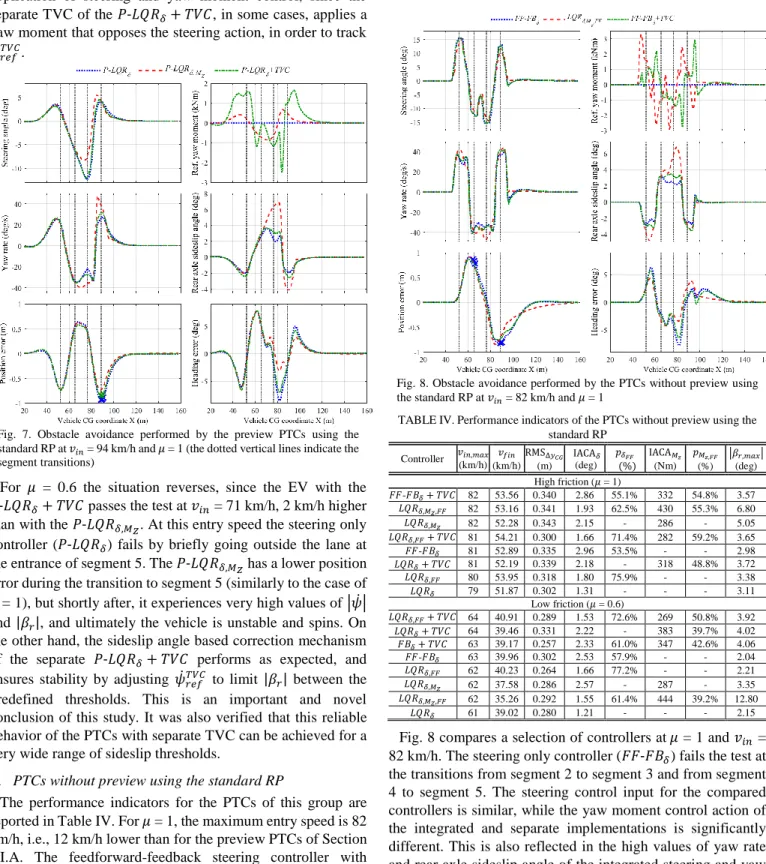
Fig. 7 reports the obstacle avoidance simulation results at 𝑣𝑖𝑛
= 94 km/h. At this speed, the 𝑃-𝐿𝑄𝑅𝛿+ 𝑇𝑉𝐶 and the 𝑃-𝐿𝑄𝑅𝛿 fail to pass the test by clipping the lane boundary at the entrance of segment 5, as indicated by the crosses in the lateral position error subplot. The results show a clear improvement of the position error for the integrated controller, 𝑃-𝐿𝑄𝑅𝛿,𝑀𝑍, at the transition between segments 4 and 5, when the EV returns to
the original lane. The EV with the 𝑃-𝐿𝑄𝑅𝛿,𝑀𝑍 experiences high values of |𝜓̇| and |𝛽𝑟|, which are a symptom of reduced
stability, and lower values of steering and yaw moment control actions. The latter can be attributed to the coordinated application of steering and yaw moment control, since the separate TVC of the 𝑃-𝐿𝑄𝑅𝛿+ 𝑇𝑉𝐶, in some cases, applies a yaw moment that opposes the steering action, in order to track 𝜓̇𝑟𝑒𝑓𝑇𝑉𝐶.
For 𝜇 = 0.6 the situation reverses, since the EV with the
𝑃-𝐿𝑄𝑅𝛿+ 𝑇𝑉𝐶 passes the test at 𝑣𝑖𝑛 = 71 km/h, 2 km/h higher
than with the 𝑃-𝐿𝑄𝑅𝛿,𝑀𝑍. At this entry speed the steering only controller (𝑃-𝐿𝑄𝑅𝛿) fails by briefly going outside the lane at the entrance of segment 5. The 𝑃-𝐿𝑄𝑅𝛿,𝑀𝑍 has a lower position
error during the transition to segment 5 (similarly to the case of 𝜇 = 1), but shortly after, it experiences very high values of |𝜓̇| and |𝛽𝑟|, and ultimately the vehicle is unstable and spins. On
the other hand, the sideslip angle based correction mechanism of the separate 𝑃-𝐿𝑄𝑅𝛿+ 𝑇𝑉𝐶 performs as expected, and
ensures stability by adjusting 𝜓̇𝑟𝑒𝑓𝑇𝑉𝐶 to limit |𝛽𝑟| between the
predefined thresholds. This is an important and novel conclusion of this study. It was also verified that this reliable behavior of the PTCs with separate TVC can be achieved for a very wide range of sideslip thresholds.
B. PTCs without preview using the standard RP
The performance indicators for the PTCs of this group are reported in Table IV. For 𝜇 = 1, the maximum entry speed is 82 km/h, i.e., 12 km/h lower than for the preview PTCs of Section VI.A. The feedforward-feedback steering controller with separate TVC (𝐹𝐹-𝐹𝐵𝛿+ 𝑇𝑉𝐶) and the integrated steering and yaw moment controllers (𝐿𝑄𝑅𝛿,𝑀𝑍 and 𝐿𝑄𝑅𝛿,𝑀𝑍,𝐹𝐹) achieve the same 𝑣𝑖𝑛,𝑚𝑎𝑥, with the additional performance indicators of
𝐽𝐴𝑠𝑠𝑒𝑠𝑠𝑚𝑒𝑛𝑡 determining the relative ranking. Fig. 6(b) shows
that the EV tracks the path with a significant delay. In contrast to the preview PTCs, the EV is not using the available space at the entrance of segments 2 and 4, as it tries to follow the RP. The EV also shows a slow convergence to the reference path, after entering segment 5.
Fig. 8. Obstacle avoidance performed by the PTCs without preview using the standard RP at 𝑣𝑖𝑛 = 82 km/h and 𝜇 = 1
TABLEIV.Performance indicators of the PTCs without preview using the standard RP Controller 𝑣(km/h) 𝑖𝑛,𝑚𝑎𝑥 𝑣𝑓𝑖𝑛 (km/h) RMSΔ𝑦𝐶𝐺 (m) IACA𝛿 (deg) 𝑝𝛿𝐹𝐹 (%) IACA𝑀𝑧 (Nm) 𝑝𝑀𝑧,𝐹𝐹 (%) |𝛽𝑟,𝑚𝑎𝑥| (deg) High friction (𝜇 = 1) 𝐹𝐹-𝐹𝐵𝛿+ 𝑇𝑉𝐶 82 53.56 0.340 2.86 55.1% 332 54.8% 3.57 𝐿𝑄𝑅𝛿,𝑀𝑍,𝐹𝐹 82 53.16 0.341 1.93 62.5% 430 55.3% 6.80 𝐿𝑄𝑅𝛿,𝑀𝑍 82 52.28 0.343 2.15 - 286 - 5.05 𝐿𝑄𝑅𝛿,𝐹𝐹+ 𝑇𝑉𝐶 81 54.21 0.300 1.66 71.4% 282 59.2% 3.65 𝐹𝐹-𝐹𝐵𝛿 81 52.89 0.335 2.96 53.5% - - 2.98 𝐿𝑄𝑅𝛿+ 𝑇𝑉𝐶 81 52.19 0.339 2.18 - 318 48.8% 3.72 𝐿𝑄𝑅𝛿,𝐹𝐹 80 53.95 0.318 1.80 75.9% - - 3.38 𝐿𝑄𝑅𝛿 79 51.87 0.302 1.31 - - - 3.11 Low friction (𝜇 = 0.6) 𝐿𝑄𝑅𝛿,𝐹𝐹+ 𝑇𝑉𝐶 64 40.91 0.289 1.53 72.6% 269 50.8% 3.92 𝐿𝑄𝑅𝛿+ 𝑇𝑉𝐶 64 39.46 0.331 2.22 - 383 39.7% 4.02 𝐹𝐵𝛿+ 𝑇𝑉𝐶 63 39.17 0.257 2.33 61.0% 347 42.6% 4.06 𝐹𝐹-𝐹𝐵𝛿 63 39.96 0.302 2.53 57.9% - - 2.04 𝐿𝑄𝑅𝛿,𝐹𝐹 62 40.23 0.264 1.66 77.2% - - 2.21 𝐿𝑄𝑅𝛿,𝑀𝑍 62 37.58 0.286 2.57 - 287 - 3.35 𝐿𝑄𝑅𝛿,𝑀𝑍,𝐹𝐹 62 35.26 0.292 1.55 61.4% 444 39.2% 12.80 𝐿𝑄𝑅𝛿 61 39.02 0.280 1.21 - - - 2.15
Fig. 8 compares a selection of controllers at 𝜇 = 1 and 𝑣𝑖𝑛 = 82 km/h. The steering only controller (𝐹𝐹-𝐹𝐵𝛿) fails the test at
the transitions from segment 2 to segment 3 and from segment 4 to segment 5. The steering control input for the compared controllers is similar, while the yaw moment control action of the integrated and separate implementations is significantly different. This is also reflected in the high values of yaw rate and rear axle sideslip angle of the integrated steering and yaw moment controller (𝐿𝑄𝑅𝛿,𝑀𝑍,𝐹𝐹), which is a consistent
characteristic of all the integrated controllers when operating at the limit of handling.
Fig. 7. Obstacle avoidance performed by the preview PTCs using the standard RP at 𝑣𝑖𝑛 = 94 km/h and 𝜇 = 1 (the dotted vertical lines indicate the segment transitions)
For 𝜇 = 0.6, the maximum entry speed of 64 km/h is achieved by the LQR controllers actuating only the steering system, in cooperation with the TVC (𝐿𝑄𝑅𝛿,𝐹𝐹+ 𝑇𝑉𝐶 and 𝐿𝑄𝑅𝛿+ 𝑇𝑉𝐶).
For example, at 𝑣𝑖𝑛= 63 km/h, the integrated steering and yaw moment controller (𝐿𝑄𝑅𝛿,𝐹𝐹) fails the test by exceeding the maneuver limits at the entrance of segment 5.
C. PTCs without preview using the smooth RP
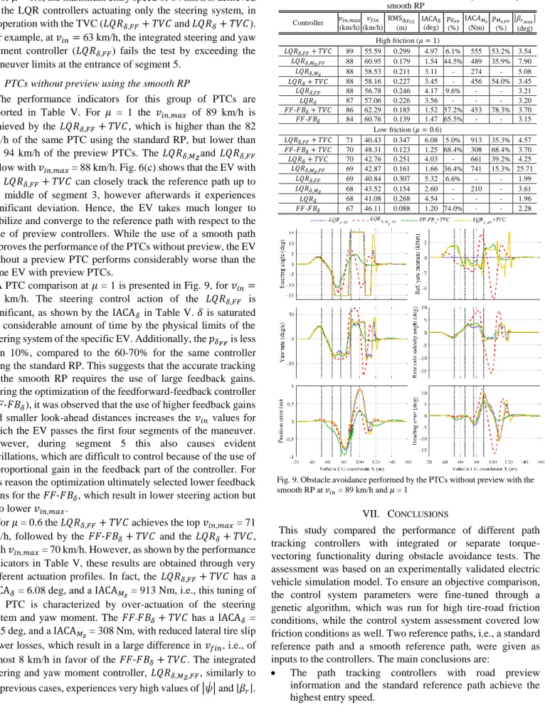
The performance indicators for this group of PTCs are reported in Table V. For 𝜇 = 1 the 𝑣𝑖𝑛,𝑚𝑎𝑥 of 89 km/h is
achieved by the 𝐿𝑄𝑅𝛿,𝐹𝐹+ 𝑇𝑉𝐶, which is higher than the 82 km/h of the same PTC using the standard RP, but lower than the 94 km/h of the preview PTCs. The 𝐿𝑄𝑅𝛿,𝑀𝑍and 𝐿𝑄𝑅𝛿,𝐹𝐹
follow with 𝑣𝑖𝑛,𝑚𝑎𝑥 = 88 km/h. Fig. 6(c) shows that the EV with
the 𝐿𝑄𝑅𝛿,𝐹𝐹+ 𝑇𝑉𝐶 can closely track the reference path up to
the middle of segment 3, however afterwards it experiences significant deviation. Hence, the EV takes much longer to stabilize and converge to the reference path with respect to the case of preview controllers. While the use of a smooth path improves the performance of the PTCs without preview, the EV without a preview PTC performs considerably worse than the same EV with preview PTCs.
A PTC comparison at 𝜇 = 1 is presented in Fig. 9, for 𝑣𝑖𝑛 =
89 km/h. The steering control action of the 𝐿𝑄𝑅𝛿,𝐹𝐹 is
significant, as shown by the IACA𝛿 in Table V. 𝛿 is saturated for considerable amount of time by the physical limits of the steering system of the specific EV. Additionally, the 𝑝𝛿𝐹𝐹 is less
than 10%, compared to the 60-70% for the same controller along the standard RP. This suggests that the accurate tracking of the smooth RP requires the use of large feedback gains. During the optimization of the feedforward-feedback controller
(𝐹𝐹-𝐹𝐵𝛿), it was observed that the use of higher feedback gains
and smaller look-ahead distances increases the 𝑣𝑖𝑛 values for
which the EV passes the first four segments of the maneuver. However, during segment 5 this also causes evident oscillations, which are difficult to control because of the use of a proportional gain in the feedback part of the controller. For this reason the optimization ultimately selected lower feedback gains for the 𝐹𝐹-𝐹𝐵𝛿, which result in lower steering action but also lower 𝑣𝑖𝑛,𝑚𝑎𝑥.
For 𝜇 = 0.6 the 𝐿𝑄𝑅𝛿,𝐹𝐹+ 𝑇𝑉𝐶achieves the top 𝑣𝑖𝑛,𝑚𝑎𝑥 = 71 km/h, followed by the 𝐹𝐹-𝐹𝐵𝛿+ 𝑇𝑉𝐶 and the 𝐿𝑄𝑅𝛿+ 𝑇𝑉𝐶,
with 𝑣𝑖𝑛,𝑚𝑎𝑥 = 70 km/h. However, as shown by the performance
indicators in Table V, these results are obtained through very different actuation profiles. In fact, the 𝐿𝑄𝑅𝛿,𝐹𝐹+ 𝑇𝑉𝐶 has a IACA𝛿 = 6.08 deg, and a IACA𝑀𝑧 = 913 Nm, i.e., this tuning of
the PTC is characterized by over-actuation of the steering system and yaw moment. The 𝐹𝐹-𝐹𝐵𝛿+ 𝑇𝑉𝐶 has a IACA𝛿 =
1.25 deg, and a IACA𝑀𝑧 = 308 Nm, with reduced lateral tire slip
power losses, which result in a large difference in 𝑣𝑓𝑖𝑛, i.e., of
almost 8 km/h in favor of the 𝐹𝐹-𝐹𝐵𝛿+ 𝑇𝑉𝐶. The integrated steering and yaw moment controller, 𝐿𝑄𝑅𝛿,𝑀𝑍,𝐹𝐹, similarly to
all previous cases, experiences very high values of |𝜓̇| and |𝛽𝑟|.
TABLEV.Performance indicators of the PTCs without preview using the smooth RP Controller 𝑣𝑖𝑛,𝑚𝑎𝑥 (km/h) 𝑣𝑓𝑖𝑛 (km/h) RMSΔ𝑦𝐶𝐺 (m) IACAδ (deg) 𝑝𝛿𝐹𝐹 (%) IAC𝐴𝑀𝑧 (Nm) 𝑝𝑀𝑧,𝐹𝐹 (%) |𝛽𝑟,max| (deg) High friction (𝜇 = 1) 𝐿𝑄𝑅𝛿,𝐹𝐹+ 𝑇𝑉𝐶 89 55.59 0.299 4.97 6.1% 555 53.2% 3.54 𝐿𝑄𝑅𝛿,𝑀𝑍,𝐹𝐹 88 60.95 0.179 1.54 44.5% 489 35.9% 7.90 𝐿𝑄𝑅𝛿,𝑀𝑍 88 58.53 0.211 3.11 - 274 - 5.08 𝐿𝑄𝑅𝛿+ 𝑇𝑉𝐶 88 58.16 0.227 3.45 - 456 54.0% 3.45 𝐿𝑄𝑅𝛿,𝐹𝐹 88 56.78 0.246 4.17 9.6% - - 3.21 𝐿𝑄𝑅𝛿 87 57.06 0.226 3.56 - - - 3.20 𝐹𝐹-𝐹𝐵𝛿+ 𝑇𝑉𝐶 86 62.29 0.185 1.52 57.2% 453 78.3% 3.70 𝐹𝐹-𝐹𝐵𝛿 84 60.76 0.139 1.47 65.5% - - 3.15 Low friction (𝜇 = 0.6) 𝐿𝑄𝑅𝛿,𝐹𝐹+ 𝑇𝑉𝐶 71 40.43 0.347 6.08 5.0% 913 35.3% 4.57 𝐹𝐹-𝐹𝐵𝛿+ 𝑇𝑉𝐶 70 48.31 0.123 1.25 68.4% 308 68.4% 3.70 𝐿𝑄𝑅𝛿+ 𝑇𝑉𝐶 70 42.76 0.251 4.03 - 661 39.2% 4.25 𝐿𝑄𝑅𝛿,𝑀𝑍,𝐹𝐹 69 42.87 0.161 1.66 36.4% 741 15.3% 25.71 𝐿𝑄𝑅𝛿,𝐹𝐹 69 40.84 0.307 5.32 6.6% - - 1.99 𝐿𝑄𝑅𝛿,𝑀𝑍 68 43.52 0.154 2.60 - 210 - 3.61 𝐿𝑄𝑅𝛿 68 41.08 0.268 4.54 - - - 1.96 𝐹𝐹-𝐹𝐵𝛿 67 46.11 0.088 1.20 74.0% - - 2.28
Fig. 9. Obstacle avoidance performed by the PTCs without preview with the smooth RP at 𝑣𝑖𝑛 = 89 km/h and 𝜇 = 1
VII. CONCLUSIONS
This study compared the performance of different path tracking controllers with integrated or separate torque-vectoring functionality during obstacle avoidance tests. The assessment was based on an experimentally validated electric vehicle simulation model. To ensure an objective comparison, the control system parameters were fine-tuned through a genetic algorithm, which was run for high tire-road friction conditions, while the control system assessment covered low friction conditions as well. Two reference paths, i.e., a standard reference path and a smooth reference path, were given as inputs to the controllers. The main conclusions are:
The path tracking controllers with road preview information and the standard reference path achieve the highest entry speed.
The use of a smooth reference path, similar to the path followed by the preview controllers, increases the maximum entry speed achievable with the controllers without preview, at the expense of increased oscillations after the vehicle returns to the original lane.
Continuously active torque-vectoring control, either with integrated or separate multi-layer implementations, improves vehicle performance compared to path tracking control only based on the steering system actuation. More specifically, torque-vectoring increases 𝑣𝑖𝑛,𝑚𝑎𝑥 by 1 to 3
km/h with respect to the EV with the same PTC, but excluding direct yaw moment control.
In the formulations without preview, the use of a feedforward contribution for steering and yaw moment actuation is usually beneficial to both the integrated and separate controllers, with an increase of 𝑣𝑖𝑛,𝑚𝑎𝑥 of up to 2 km/h.
The integrated steering and yaw moment controllers can achieve high entry speeds, and thus enhanced vehicle agility, especially if they include a preview component in their formulation, and are tuned for the specific tire-road friction condition. Therefore, the integrated control structures can be recommended for race vehicle applications, such as the EV of this study, which operates on race tracks, with at least approximately known friction conditions. However, the integrated solutions tend to give origin to very variable behavior when they operate at different friction coefficients. In particular, the integrated controllers provoked very high values of |𝛽𝑟| in many of the tests at 𝜇 = 0.6, because of the intrinsic lack of consideration of vehicle stability and cornering limits in their formulations.
The separate TVC guarantees consistently safe and stable EV response, with |𝛽𝑟| saturation according to the
specified thresholds. Based on these results, the multi-layer control structures are recommended for future passenger car implementations. As a consequence, the wide literature already available on the topic of torque-vectoring control of human-driven EVs with multiple motors remains meaningful and valid also for the design of TVCs for autonomous EVs.
The next steps of this research will be focused on the experimental validation of these simulation results and the analysis of the effect of parameter uncertainties and disturbances.
REFERENCES
[1] A. Sorniotti, P. Barber, and S. De Pinto, “Path Tracking for Automated Driving: A Tutorial on Control System Formulations and Ongoing Research,” in Automated driving: Safer and More Efficient Future
Driving, D. Watzenig and M. Horn, Springer, pp. 71–140, 2017.
[2] C. Chatzikomis and K.N. Spentzas, “A path-following driver model with longitudinal and lateral control of vehicle’s motion,” Forsch. im
Ingenieurwesen/Engineering Res., vol. 73, no. 4, pp. 257–266, 2009.
[3] J. Edelmann, M. Plöchl, W. Reinalter, and W. Tieber, “A passenger car driver model for higher lateral accelerations,” Veh. Syst. Dyn., vol. 45, no. 12, pp. 1117–1129, 2007.
[4] C.C. MacAdam, “Application of an Optimal Preview Control for Simulation of Closed-Loop Automobile Driving,” IEEE Trans. Syst.
Man. Cybern., vol. 11, no. 6, pp. 393–399, 1981.
[5] G. Markkula, O. Benderius, K. Wolff, and M. Wahde, “A Review of Near-Collision Driver Behavior Models,” Hum. Factors J. Hum. Factors
Ergon. Soc., vol. 54, no. 6, pp. 1117–1143, 2012.
[6] M. Plöchl and J. Edelmann, “Driver models in automobile dynamics application,” Veh. Syst. Dyn., vol. 45, no. 7–8, pp. 699–741, 2007. [7] R.S. Sharp, D. Casanova, and P. Symonds, “A Mathematical Model for
Driver Steering Control, with Design, Tuning and Performance results,”
Veh. Syst. Dyn., vol. 33, pp. 289–326, 2000.
[8] R. Attia, R. Orjuela, and M. Basset, “Combined longitudinal and lateral control for automated vehicle guidance,” Veh. Syst. Dyn., vol. 52, no. 2, pp. 261–279, 2014.
[9] A. Carvalho, S. Lefévre, G. Schildbach, J. Kong, and F. Borrelli, “Automated driving: The role of forecasts and uncertainty—A control perspective,” Eur. J. Control, vol. 24, pp. 14–32, 2015.
[10] P. Falcone, F. Borrelli, J. Asgari, H.E. Tseng, and D. Hrovat, “Predictive Active Steering Control for Autonomous Vehicle Systems,” IEEE Trans.
Control Syst. Technol., vol. 15, no. 3, pp. 566–580, 2007.
[11] K. Kritayakirana and J.C. Gerdes, “Using the centre of percussion to design a steering controller for an autonomous race car,” Veh. Syst. Dyn.,
vol. 50, no. sup. 1, pp. 33–51, 2012.
[12] G. Tagne, R. Talj, and A. Charara, “Higher-order sliding mode control for lateral dynamics of autonomous vehicles, with experimental validation,” IEEE Intelligent Vehicles Symposium, Proc., pp. 678–683, 2013.
[13] S. Thrun et al., “Stanley: The robot that won the DARPA Grand Challenge,” Springer Transacts. Adv. Robot., vol. 36, pp. 1–43, 2007. [14] F. Roselli et al., “H-infinity control with look-ahead for lane keeping in
autonomous vehicles,” 2017 IEEE Conference on Control Technology
and Applications (CCTA 2017), Proc., pp. 2220-2225, 2017.
[15] J.M. Snider, “Automatic Steering Methods for Autonomous Automobile Path Tracking,” CMU-RI-TR-09-08, Report, Carnegie Mellon University, 2009.
[16] L. De Novellis et al., “Direct yaw moment control actuated through electric drivetrains and friction brakes: Theoretical design and experimental assessment,” Mechatronics, vol. 26, pp. 1–15, 2015. [17] Q. Lu et al.,“Enhancing vehicle cornering limit through sideslip and yaw
rate control,” Mech. Syst. Signal Process., vol. 75, pp. 455–472, 2016. [18] M. Canale, L. Fagiano, A. Ferrara, and C. Vecchio, “Comparing Internal
Model Control and Sliding Mode Approaches for Vehicle Yaw Control,”
IEEE Trans. Intell. Transp. Syst., vol. 10, no. 1, pp. 31–41, 2009.
[19] T. Goggia et al., “Integral Sliding Mode for the Torque-Vectoring Control of Fully Electric Vehicles: Theoretical Design and Experimental Assessment,” IEEE Trans. Veh. Technol., vol. 64, no. 5, pp. 1701–1715, 2014.
[20] J.S. Hu, Y. Wang, H. Fujimoto, and Y. Hori, “Robust Yaw Stability Control for In-Wheel Motor Electric Vehicles,” IEEE/ASME Trans.
Mechatr., vol. 22, no. 3, pp. 1360–1370, 2017.
[21] H. Fujimoto and K. Maeda, “Optimal yaw-rate control for electric vehicles with active front-rear steering and four-wheel driving-braking force distribution, 39th Annual Conference of the IEEE Industrial
Electronics Society, Proc., pp. 6514–6519, 2013.
[22] M. Corno, M. Tanelli, I. Boniolo, and S.M. Savaresi, “Advanced yaw control of four-wheeled vehicles via rear active differential steering,”
48th IEEE Conference on Decision and Control (CDC) and 2009 28th
Chinese control Conference, Proc., pp. 5176–5181, 2009.
[23] R. de Castro, M. Tanelli, R.E. Araújo, and S.M. Savaresi, “Minimum-time manoeuvring in electric vehicles with four wheel-individual-motors,” Veh. Syst. Dyn., vol. 52, no. 6, pp. 824–846, 2014.
[24] C. Chatzikomis, A. Sorniotti, P. Gruber, M. Bastin, R. M. Shah, and Y. Orlov, “Torque-Vectoring Control for an Autonomous and Driverless Electric Racing Vehicle with Multiple Motors,” SAE Int. J. Veh. Dyn.,
Stab., NVH, vol. 1, no. 2, pp. 338–351, 2017.
[25] S.T. Peng, C.C. Hsu, and C.C. Chang, “On a robust bounded control design of the combined wheel slip for an autonomous 4WS4WD ground vehicle,” Veh. Syst. Dyn., vol. 2005, no. 5, pp. 6504–6509, 2005. [26] H. Okajima, S. Yonaha, N. Matsunaga, and S. Kawaji, “Direct
Yaw-moment Control method for electric vehicles to follow the desired path by driver,” SICE Annual Conf. 2010, Proc., pp. 642–647, 2010. [27] R. Wang, C. Hu, F. Yan, and M. Chadli, “Composite Nonlinear Feedback
Control for Path Following of Four-Wheel Independently Actuated Autonomous Ground Vehicles,” IEEE Trans. Intell. Transp. Syst., vol. 17, no. 7, pp. 2063–2074, 2016.
[28] B. Li, H. Du, and W. Li, “A Potential Field Approach-Based Trajectory Control for Autonomous Electric Vehicles With In-Wheel Motors,”
[29] C. Hu, R. Wang, F. Yan, and N. Chen, “Output Constraint Control on Path Following of Four-Wheel Independently Actuated Autonomous Ground Vehicles,” IEEE Trans. Veh. Technol., vol. 65, no. 6, pp. 4033– 4043, 2016.
[30] A. Goodarzi, A. Sabooteh, and E. Esmailzadeh, “Automatic path control based on integrated steering and external yaw-moment control,” Proc.
Inst. Mech. Eng. Part K J. Multi-body Dyn., vol. 222, no. 2, pp. 189–
200, 2008.
[31] P. Falcone, H. Eric Tseng, F. Borrelli, J. Asgari, and D. Hrovat, “MPC-based yaw and lateral stabilisation via active front steering and braking,”
Veh. Syst. Dyn., vol. 46, no. sup1, pp. 611–628, 2008.
[32] F. Yakub and Y. Mori, “Comparative study of autonomous path-following vehicle control via model predictive control and linear quadratic control,” Proc. Inst. Mech. Eng. Part D J. Automob. Eng., vol. 229, no. 12, pp. 1695–1714, 2015.
[33] International Standards Organisation, “Passenger cars — Test track for a severe lane-change manoeuvre Part 2 : Obstacle avoidance.” ISO 3888-2:2011, 2011.
[34] N.R. Kapania and J.C. Gerdes, “Design of a feedback-feedforward steering controller for accurate path tracking and stability at the limits of handling,” Veh. Syst. Dyn., vol. 53, no. 12, pp. 1687–1704, 2015. [35] Q. Lu, A. Sorniotti, P. Gruber, J. Theunissen, and J. De Smet, “H∞ loop
shaping for the torque-vectoring control of electric vehicles: Theoretical design and experimental assessment,” Mechatronics, vol. 35, pp. 32–43, 2016.
[36] E. Ostertag, Mono-and Multivariable Control and Estimation, Springer, 2011.
[37] R.S. Sharp and V. Valtetsiotis, “Optimal preview car steering control,”
ICTAM Sel. Pap. from 20th Int. Cong., Proc., pp. 101–117, 2001.
[38] B. Lenzo, A. Sorniotti, P. Gruber, and K. Sannen, On the experimental analysis of single input single output control of yaw rate and sideslip angle, Int. J. Autom. Technol., vol. 18, no. 5, pp. 799-811, 2017. [39] M. Jalali, E. Ashemi, A. Khajepour, S. Chen, and B. Litkouhi,
“Integrated model predictive control and velocity estimation of electric vehicles,” Mechatronics, vol. 46, pp. 84-100, 2017.
[40] M. Gobbi, I. Haque, P.Y. Papalambros, and G. Mastinu, “Optimization and integration of ground vehicle systems,” Veh. Syst. Dyn., vol. 43, no. 6–7, pp. 437–453, 2005.
[41] H. Haghiac, I. Haque, and G. Fadel, “An assessment of a genetic algorithm-based approach for optimising multi-body systems with applications to vehicle handling performance,” Int. J. Veh. Des., vol. 36, no. 4, pp. 320–344, 2004.
[42] H.G. Beyer, The theory of evolution strategies, Springer, 2013.
Christoforos Chatzikomis received the M.Sc. and
Ph.D. degrees in mechanical engineering from the National Technical University of Athens, Athens, Greece, in 2003 and 2010, respectively. Between 2015 and 2017, he was a Research Fellow in electric vehicle control with the University of Surrey, Guildford, U.K. Since 2018 he has been working as a Control Systems Engineer for Roborace. His main research interests include vehicle dynamics, electric vehicle control, and autonomous vehicles.
Aldo Sorniotti (M’12) received the M.Sc. degree in
mechanical engineering and Ph.D. degree in applied mechanics from the Politecnico di Torino, Turin, Italy, in 2001 and 2005, respectively. He is a Professor in advanced vehicle engineering with the University of Surrey, Guildford, U.K., where he coordinates the Centre for Automotive Engineering. His research interests include vehicle dynamics control and transmission systems for electric and hybrid vehicles.
Patrick Gruber received the M.Sc. degree in
motorsport engineering and management from Cranfield University, Cranfield, U.K., in 2005, and the Ph.D. degree in mechanical engineering from the University of Surrey, Guildford, U.K., in 2009. He is a Senior Lecturer in advanced vehicle systems engineering with the University of Surrey. His current research interests include vehicle and tire dynamics, and the development of novel tire and rubber friction models.
Mattia Zanchetta received the B.Sc. degree in
electronic engineering and telecommunications and the M.Sc. degree in control engineering from the University of Pavia, Pavia, Italy, in 2013 and 2016, respectively. He is now a PhD researcher at the University of Surrey, Guildford, U.K. His current research interests include vehicle dynamics control, vehicle testing and autonomous driving.
Bryn Balcombe is the Chief Technology Officer for
Roborace, the world’s first driverless electric racing series. He received a degree in mechanical engineering and vehicle design from the University of Hertfordshire, Hatfield, U.K., in 1996. His experience spans 16 years working for Bernie Ecclestone’s Formula One Management leading all significant technical projects from the construction of new circuits to fully automated cars and camera tracking systems, and the implementation of the Formula One Global Media Network. He left to join the executive team of a media start up pioneering multiple cutting edge technologies for TV studios and has also consulted on technology strategy for organisations including the BBC and McCann Worldgroup.
Dan Willans received the M.Eng. degree in
mechanical engineering from the University of Surrey, Guildford, U.K., in 2016. Since July 2016 he has been working as a Control Systems Engineer with Roborace. His main activities include delivering software and hardware solutions for the vehicles developed by Roborace.