DOTTORATO DI RICERCA IN
Automatica e Ricerca Operativa
Ciclo XXVIII
Settore concorsuale di afferenza: 01/A6 - RICERCA OPERATIVA Settore scientifico disciplinare: MAT/09 - RICERCA OPERATIVA
Models and Solutions of Resource
Allocation Problems based on Integer
Linear and Nonlinear Programming
Presentata da:
Dimitri Thomopulos
Coordinatore Dottorato
Relatore
Prof. Daniele Vigo
Prof. Enrico Malaguti
Correlatore
Prof. Andrea Lodi
1 Introduction 1
1.1 On Resource Allocation Problems. . . 1
1.2 Thesis Contribution . . . 4
1.3 Applied Motivations . . . 5
1.4 Thesis Methodological Outline . . . 6
1.4.1 Two-Dimensional Guillotine Cutting Problem . . . 6
1.4.2 Mid-Term Hydro Scheduling Problem . . . 7
2 Two-Dimensional Guillotine Cutting Problem 11 2.1 Introduction. . . 11
2.1.1 Families of cutting problems. . . 12
2.1.2 Structure of general guillotine cuts. . . 13
2.1.3 Literature review. . . 13
2.1.4 Contribution. . . 16
2.2 MIP modeling of guillotine cuts . . . 16
2.2.1 Definition of the cut position set . . . 20
2.2.2 Model extensions: Cutting Stock problem and Strip Packing problem . . . 25
2.3 An effective solution procedure for thePP-G2KP Model . . . 27
2.3.1 Variable pricing procedures . . . 27
2.4 Computational Experiments . . . 29
2.4.1 Lower bound (feasible solution) computation . . . 32
2.4.2 Iterative Variable Pricing . . . 34
2.4.3 Models size and reductions . . . 36
2.4.4 Overall solution procedure. . . 41
2.4.5 Comparison with state-of-the-art approaches . . . 46
2.4.6 Relevance of guillotine cuts . . . 48
2.5 Conclusions . . . 49
3 Mid-Term Hydro Scheduling Problem 51 3.1 Introduction. . . 51
3.1.1 Mid-term hydro scheduling . . . 54
3.1.2 Choice of the objective function. . . 55
3.2 Decomposition algorithm for nonlinear (CCP) . . . 56
3.2.1 Overview of the approach . . . 58
3.2.2 Separation algorithm . . . 59
3.3.1 Decomposition . . . 67
3.3.1.1 Electricity generation function . . . 68
3.3.1.2 Demand and price function . . . 69
3.3.2 Data . . . 69
3.4 Computational experiments . . . 71
3.4.1 Implementation details. . . 71
3.4.2 Computational performance . . . 73
3.4.3 Quadratic electricity generation function. . . 80
3.4.4 The effect ofα on the profit . . . 84
3.4.5 Other solvers . . . 86
3.5 Conclusions . . . 90
• Two-dimensional Cutting Problems • Guillotine Knapsack Problems • Chance Constrained Programming • Exact Algorithms
• Integer Linear Programming • Nonlinear Programming • Pricing
• Stochastic Programming • Computational Experiments
I want to express my deeply-felt thanks to my thesis advisors, Professors Enrico Malaguti and Andrea Lodi, for their warm encouragement, thoughtful guidance. I also want to express my gratitude to Dr.Valentina Cacchiani for her continuous support and sound advice.
Introduction
1.1
On Resource Allocation Problems
Resource Allocation is the generic problem of assigning available resources to users in the best possible way. Usually the resources are limited, thus sets of activities compete for these resources establishing explicit and implicit dependencies, which may be subject to uncertainty. The resulting decision problem on the best use of the resources can be be decomposed in several problems that have been intensively studied in the field of operations research in the last few decades. Examples of such problems are:
• Scheduling Problem. Scheduling is the process of deciding, controlling and optimizing works and activities in a production process or manufacturing process. Scheduling is used to optimally allocate scarce resources to activities, and includes problems like the allocation of plant and machinery resources, the organization of human resources, and the control of production processes and materials purchase (see, e.g., Jordan [1996]).
• Knapsack Problem. A large variety of resource allocation problems can be cast in the framework of a knapsack problem. The aim of this problem, given a set of items, each with a weight and a profit, is to maximize the total obtained value, determining the number of each item to include in a knapsack, or more generally in a collection, so that the total weight is less than or equal to a given limit. The main idea is to consider the capacity of the knapsack as the available amount of resource and the item types as activities to which this resource can be allocated (see, e.g., Martello and Toth[1990]).
• Cutting Stock Problem. CSP is a general resource allocation problem where the objective is to cut pieces of stock material into pieces of specified sizes, minimizing the wasted material. Focusing more on the resources it can be defined
as the decision of subdividing a given amount of a resource into a number of predetermined allocations so that the left-over amount is minimized (see, e.g., Gilmore and Gomory[1961]).
• Power Generation Scheduling Problem. Power Generation Scheduling is required in order to find the optimum allocation of energy such that the annual operating cost of a power system is minimized, or the obtained profit is maximized (see, e.g., Bertsekas et al. [1983]). This problem is also strictly related to the Unit Commitment Problem or Pre-Dispatch Problem, and it has been subject to considerable discussion in the power system literature.
There is a large literature dealing with these problems and several solving techniques have been proposed. One of the most widely used modeling and solution techniques is Mathematical Programming (MP). This is one of the most effective and it can be conveniently defined as a mathematical representation aimed at programming, i.e., planning the best possible allocation of scarce resources. Many real-world and theo-retical resource allocation problems may be modeled in this general framework, which involves searching for the optimal settings of decision variables satisfying all the occur-ring constraints, while optimizing the objective function. These constraints represent the conditions, like financial, technological and organizational conditions, which occur in the problem.
Mathematical Programming is a significantly large discipline and several subfields have been explored specifically. Among them we can mention:
• Linear Programming, LP in short, is a modeling technique for achieving the best objective function in a mathematical model characterized by linear functions. Hence, the objective function is linear and the constraints are linear inequalities (see, e.g., Luenberger and Ye[2008]).
The first Linear Programming formulation of a problem was given by Kantorovich in 1939, who also proposed a method for solving it (see, e.g., Schrijver [1986]). He developed it during World War II motivated by combinatorial applications, in particular transportation and transshipment. About the same time as Kan-torovich, also Koopmans introduced LPs, formulating classical economic prob-lems as Linear Programs. In addition, during 1946-1947, Dantzig independently developed the General Linear Programming formulation. He was working for the United States Air Force, where one of his tasks was to develop mathematical models that could be used to formulate practical planning and scheduling prob-lems. In 1947, Dantzig also invented the Simplex Method that is the most widely applied algorithm for solving Linear Problems. In fact the journal Computing in Science and Engineering listed it as one of the top 10 algorithms of the twentieth century.
A convenient expression of LP is
(LP) maxf(x) (1.1)
g(x)≤0 (1.2)
x∈Rn+ (1.3)
• Integer Programming IP in short, refers to the class of constrained optimiza-tion problems in which the variables are required to be integers. In many settings the term refers to Integer Linear Programming (ILP), in which the objective func-tion is linear and the constraints are linear inequalities (see, e.g., J¨unger et al. [2010]).
A generic ILP is conveniently expressed as
(ILP) maxf(x) (1.4)
g(x)≤0 (1.5)
x∈Zn (1.6)
0-1 Linear Programming is a possible special case of ILP that involves only binary variables, i.e. variables that are restricted to be either 0 or 1. A generalization is Mixed-Integer Linear Programming (MILP) that involves problems in which only some of the variablesx, are constrained to be integers, while other variables are allowed to be non-integers.
Linear and Integer Linear Programming are presented, e.g., in Bertsimas and Tsitsiklis [1997], Papadimitriou and Steiglitz[1998].
• Nonlinear Programming, NLP in short, is a framework for modeling prob-lems defined by constraints, over a set of real variables, along with an objective function to be maximized or minimized, where some of the constraints or the objective function are nonlinear (see, e.g., Luenberger and Ye[2008]).
A NLP is conveniently expressed as
(NLP) maxf(x) (1.7)
g(x)≤0 (1.8)
x∈X⊆Rn (1.9)
where g(x) is a nonlinear function.
Similarly to the ILP approach it is possible to consider a variant of NLP where some of the variables x are constrained to be integers, while other variables are allowed to be non-integers. This is the Mixed-Integer Nonlinear Programming (MINLP) approach.
• Stochastic Programming. Stochastic Programs are mathematical programs for modeling problems that involve uncertainty. Uncertainty is usually char-acterized by a probability distribution on the model parameters. Some of the data incorporated into the objective function or the constraints are uncertain, and if some of the data are random, then also the solutions and the optimal objective values are themselves random. In order to deal with uncertainties in optimization, the available stochastic information is integrated into the problem formulation.
One possible way for representing these problems is using recursive models, that take one decision now and minimize the expected costs (or utilities) of the con-sequences of that decision. Let us assume to have a set of decisions to be taken without full information on some random events represented by a vectorx. These decisions are called first-stage decisions. Later, full information is received on the realization of some random vectorξ. Then, some corrective actionycan be taken. These decisions are called second-stage decisions. This is known in literature as the Two-Stage Stochastic Program (see, e.g., Birge and Louveaux [1997]). A convenient expression of Two-Stage Stochastic Program is
(2S−SP) maxf(x) +E[Q(x, ξ)] (1.10)
g(x)≤0 (1.11)
x∈X (1.12)
where Q(x,ξ) is the minimized expected cost.
In some cases, it may be more appropriate to try to find a decision that ensures that the probability of meeting a set of certain constraints is above a certain level. This is the case of Chance-Constrained Programming, first introduced by Charnes et al. [1958].
A generic formulation of Chance-Constrained Programming problem is
(CCP) maxf(x, ξ) (1.13) g(x, ξ)≤0 (1.14) P(g(x, ξ)≥0)≥p (1.15) x∈X (1.16) p∈[0,1] (1.17)
1.2
Thesis Contribution
In this thesis we deal with some variants of these approaches used for solving the con-sidered resource allocation problems. In the first part we focus on the Integer Program-ming approach for solving Two-Dimensional Guillotine Cutting Problems. We propose
a new framework to model general guillotine restrictions through a Mixed-Integer Lin-ear Formulation. In the second part we present a Branch-and-Cut algorithm for a class of Nonlinear Chance Constrained Mathematical Optimization Problems with a finite number of scenarios. We apply this algorithm to a specific Power Generation Schedul-ing Problem, i.e., the Mid-Term Hydro SchedulSchedul-ing Problem, for which we propose a chance-constrained formulation. Thus, we propose a sophisticated algorithmic com-bination of the three approaches Integer Programming, Nonlinear Programming and Stochastic Programming specifically tailored for solving resource allocation problems with a practical impact. Table 1.1summarizes the combined approaches.
LP ILP N LP CCP Two-Dimensional Guillotine Cutting Problem yes yes no no Mid-Term Hydro Scheduling Problem no yes yes yes
Table 1.1: Used approaches
1.3
Applied Motivations
Making decisions on issues with important consequences has become a highly complex problem due to the many competing forces under which the world is operating today. Operations Research and Mathematical Programming techniques have been used more and more to support managerial decisions. In this thesis we consider Two-Dimensional Guillotine Cutting Problems and the Mid-Term Hydro Scheduling Problem. They be-long to some of the current and crucial class of problems in which Mathematical Pro-gramming is applied.
The study of efficient and innovative methods for solving Cutting Problems is required by the economic impact of such problems. They are of great relevance in metal, wood, paper or glass industries, but also in loading, transportation, telecommunications and resource allocation in general (see, e.g., Bennell et al. [2013], Burke et al. [2006], Iori et al. [2007], Lodi et al. [2011],Malaguti et al.[2014],Vanderbeck [2001]). Depending on the industry, special features for the cuts may be required. Usingguillotine cuts is one of the most common of them. It applies to wood cutting, and in particular to glass cutting. Glass Alliance Europe [2015] estimated that in 2014 the EU-28 glass produc-tion reached a volume of more than 33 million tonnes, a slight increase of 2% compared with 2013, involving 180,000 employees. This production level still maintains the EU as the largest glass producer in the world with a market share of around 33% of the total world market. Several industrial sectors directly depend on the production of glass. Indeed, some of the most important customers of glass industries come from the car industry, the construction sector, domestic and leisure industries. Therefore, even small savings in costs may have a relevant global impact.
The other crucial problem studied in this thesis belongs to the family of the Power Generation Scheduling Problems. Electric power today plays an exceedingly impor-tant role in the development of several economic sectors, but also in the most common aspects of modern life. Indeed, the modern economy is completely dependent on the electric power, which is one of the basic inputs of several activities. With the ever in-creasing per capita energy consumption and exponentially rising population, also the need for power stations, transmission lines and networks is increasing. Consequently Power Generation Scheduling Problems are becoming more and more complex and relevant. The International Energy Agency [2015] estimated that in 2013 the world energy consumption was 13,541 Mtoe, or 1.6×10¹¹MWh. Hydroelectricity is the most widely used form of renewable energy, accounting for 3.9×10⁹ MWh of production in 2013, with the generation costs that fall into a range of 50 to 100 USD/MWh. Not surprisingly Power Generation Scheduling Problems deal with resources worth millions of dollars. Thus, it is fundamental to optimize the activities that concern power pro-duction.
1.4
Thesis Methodological Outline
In §1.2 we presented the practical contents of the thesis, instead in this Section we present the methodological contents and contributions. As we mentioned before, in this thesis we deal with two problems of resource allocation solved through a Mixed-Integer Linear Programming approach and a Mixed-Mixed-Integer Nonlinear Chance Con-straint Programming approach, which are combinations of the approaches described in§1.1:
• Two-Dimensional Guillotine Cutting Problem, • Mid-Term Hydro Scheduling Problem.
1.4.1 Two-Dimensional Guillotine Cutting Problem
Cutting Problems are combinatorial optimization problems, which occur in several real-world applications of industry and production. Due to the complexity and extensive nature of these problems, several different formulations and approaches have been proposed in literature (see, e.g., Bennell et al. [2013], Burke et al. [2006], Dyckhoff [1981],Gilmore and Gomory[1961],Iori et al.[2007],Lodi et al.[2011],Malaguti et al. [2014],Vanderbeck[2001]). The countless existing variants differ in terms of dimension, application field and special requirements. Two Dimensional Cutting Problems are subsets of these possible variants, which concern the best method to obtain a set of small (rectangular) items from one or more (rectangular) largerpanels. Depending on
the industry, special features for the cuts may be required; a very common one which applies to glass and wood cutting is to have guillotine cuts.
(i) In guillotine cutting, items are obtained from panels through cuts that are parallel to the sides of the panel and cross the panel from one side to the other;
(ii) Cuts can be performed in stages, where each stage consists of a set of parallel guillotine cuts on the shapes obtained in the previous stages. If the maximum number of stages is not allowed to exceed a valuen, the problem is calledn−stage. Otherwise, if there is no such restriction the problem is called non−stage;
(iii) Each cut removes a so-called strip from a panel. If during the cut sequence, the width of each cut strip equals the width of the widest item obtained from the strip, then the cut is denoted as restricted.
In Chapter 2, we propose a framework to model general guillotine restrictions in two-dimensional cutting problems formulated as Mixed-Integer Linear Programs (MILP). The modeling framework requires a pseudo-polynomial number of variables and con-straints, which can be effectively enumerated for medium-size instances. Our modeling of general guillotine cuts is the first one that, once it is implemented within a state-of-the-art MIP solver, can tackle instances of challenging size. Our objective is to propose a way of modeling general guillotine cuts via Mixed Integer Linear Programs (MILP), i.e., we do not limit the number of stages (restriction (ii)), nor impose the cuts to be restricted (restriction (iii)). We only ask the cuts to be guillotine ones (re-striction (i)). We mainly concentrate our analysis on the Guillotine Two Dimensional Knapsack Problem (G2KP), for which a model, and an exact procedure able to sig-nificantly improve the computational performance, are given. We also show how the modeling of general guillotine cuts can be extended to other relevant problems such as the Guillotine Two Dimensional Cutting Stock Problem (G2CSP) and the Guillotine Strip Packing Problem (GSPP). Finally, we conclude the Chapter discussing an exten-sive set of computational experiments on G2KP and GSPP benchmark instances from the literature.
1.4.2 Mid-Term Hydro Scheduling Problem
Mathematical Programming is an invaluable approach for optimal decision-making that was initially developed in a deterministic setting. However, early studies on prob-lems with probabilistic (i.e., nondeterministic) constraints have appeared since the late 50s, see, e.g., Charnes et al. [1958], Prekopa [1970]. In a problem with probabilistic constraints the formulation involves a (vector-valued) random variable that parame-terizes the feasible region of the problem; the decisionmaker specifies a probability α, and the solution to the problem must maximize a given objective function subject to
being inside the feasible region for a set of realizations of the random variable that occurs with probability at least 1−α. The interpretation is that a solution that does not belong to the feasible region is undesirable, and we want this event to happen with small probability α. This type of problem is a Chance Constrained Mathemati-cal Programming problem. For convenience, we reformulated the Chance Constrained Mathematical Program (1.13)-(1.17) as
(CCP) maxf(x, ξ) (1.18)
g(x, ξ)≤0 (1.19)
P(g(x, ξ)≥0)≥1−α (1.20)
x∈X (1.21)
The main application of Chance-Constrained Programming studied in this thesis is the Mid-Term Hydro Scheduling Problem. A central problem in power generation systems is that of optimally planning resource utilization in the mid and long term and in the presence of uncertainty. Hydro power production networks usually consist of several reservoir systems, often interconnected, which are operated on a yearly basis: it is common to have seasonal cycles for demand and inflows, which can be out of phase by a few months, i.e. inflow peaks typically precede demand peaks by a few months. The Mid-Term Hydro Scheduling Problem refers to the problem of planning produc-tion over a period of several months. To be effective, such planning must take into account uncertainty affecting rainfall and energy demand, as well as the complex and nonlinear power production functions. A commonly used approach in practice is to rely on deterministic optimization tools and on the experience of domain experts to deal with the uncertainty, because of the sheer difficulty of incorporating uncertainty into the model. Many deterministic approaches can be found in the literature, see, e.g., Carneiro et al. [1990]. More recently, methodologies that can take into account the uncertainty in the model have appeared, see, e.g., Carpentier et al. [2012], but these are still rare compared to the deterministic ones.
In Chapter 3, we present a Branch-and-Cut algorithm for a class of Nonlinear Chance Constrained Mathematical Optimization Problems with a finite number of scenarios. This class corresponds to the problems that can be reformulated as Deterministic Con-vex Mixed-Integer Nonlinear Programming problems, but the size of the reformulation is large and quickly becomes impractical as the number of scenarios grows. The Branch-and-Cut algorithm is based on an implicit Benders decomposition scheme (see, e.g., Geoffrion[1972]), where we generate cuts as outer approximation cuts from the projec-tion of the feasible region on suitable subspaces. The size of the master problem in our scheme is much smaller than the deterministic reformulation of the chance-constrained problem. We apply the Branch-and-Cut algorithm to the Mid-Term Hydro Scheduling Problem, for which we propose a chance-constrained formulation. We are not aware
of previous work that employs a chance-constrained formulation for the mid-term hy-dro scheduling problem, although there has been work on the related unit commitment problem, see, e.g.,van Ackooij[2014],Wang et al.[2012]. Even in the case of unit com-mitment, chance-constrained optimization approaches are the least commonly used in the literature, due to their difficulty [Tahanan et al.,2015, Sect. 4.4]. A computational study using data from ten hydro plants in Greece shows that the proposed methodol-ogy solves instances orders of magnitude faster than applying a general-purpose solver for Convex Mixed-Integer Nonlinear Problems to the deterministic reformulation, and scales much better with the number of scenarios. Our numerical experiments show that introducing a small amount of flexibility in the formulation, by allowing constraints to be violated with a joint probability ≤5%, increases the expected profit by 6.1%.
Two-Dimensional Guillotine
Cutting Problem
1
In this chapter we propose a framework to model general guillotine restrictions in two-dimensional cutting problems formulated as Mixed Integer Linear Programs (MIP). The modeling framework requires a pseudo-polynomial number of variables and con-straints, which can be effectively enumerated for medium-size instances. Our modeling of general guillotine cuts is the first one that, once it is implemented within a state-of-the-art MIP solver, can tackle instances of challenging size. We mainly concentrate our analysis on the Guillotine Two Dimensional Knapsack Problem (G2KP), for which a model, and an exact procedure able to significantly improve the computational per-formance, are given. We also show how the modeling of general guillotine cuts can be extended to other relevant problems such as the Guillotine Two Dimensional Cutting Stock Problem (G2CSP) and the Guillotine Strip Packing Problem (GSPP). Finally, we conclude the Chapter discussing an extensive set of computational experiments on G2KP and GSPP benchmark instances from the literature.
2.1
Introduction
Two dimensional cutting problems are about obtaining a set of small (rectangular) items from one or more (rectangular) largerpanels. Cutting problems are of great rel-evance in metal, wood, paper or glass industries, but also in loading, transportation, telecommunications and resource allocation in general (see, e.g., Bennell et al.[2013], Burke et al.[2006],Iori et al. [2007],Lodi et al.[2011],Malaguti et al.[2014], Vander-beck[2001]). Depending on the industry, special features for the cuts may be required; a very common one which applies to glass and wood cutting is to haveguillotine cuts.
1
This chapter is based onFurini et al.[2014] 11
Figure 2.1: Examples of patterns which can be obtained through: non-guillotine cuts (left), three-stage restricted guillotine cuts (center), guillotine cuts (right).
(i) In guillotine cutting, items are obtained from panels through cuts that are parallel to the sides of the panel and cross the panel from one side to the other;
(ii) Cuts are performed in stages, where each stage consists of a set of parallel guil-lotine cuts on the shapes obtained in the previous stages;
(iii) Each cut removes a so-called strip from a panel. If during the cut sequence, the width of each cut strip equals the width of the widest item obtained from the strip, then the cut is denoted as restricted.
Our objective is to propose a way of modeling general guillotine cuts via Mixed Integer Linear Programs (MIPs), i.e., we do not limit the number of stages (restriction (ii)), nor impose the cuts to be restricted (restriction (iii)). We only ask the cuts to be guillotine ones (restriction (i)). In the following, we call these kind of cuts general guillotine cuts or simplyguillotine cuts.
In Figure2.1we report, on the left, a pattern (cutting scheme) that cannot be obtained through guillotine cuts, in the center, a pattern that can be obtained through three-stage restricted guillotine cuts, and in the right a pattern that needs unrestricted guillotine cuts to be obtained, which are the ones we are interested in.
2.1.1 Families of cutting problems.
In the following, we will mainly concentrate our analysis on the Two Dimensional Knapsack Problem, and briefly discuss extensions of the modeling ideas to the Two Dimensional Cutting Stock Problem and the Strip Packing Problem. For convenience, we remind the definition of these problems.
• Two-Dimensional Knapsack Problem (2KP): we are given one rectangular panel of length L and width W, and a list of n rectangular items; each item i (i = 1, . . . , n) is characterized by a length li, a width wi, a profitpi, and is available inui copies. The 2KP requires to cut the subset of items of largest profit which can fit in the rectangular panel (without overlapping).
• Two-Dimensional Cutting Stock Problem (2CSP): we are given infinitely many identical rectangular panels, each one having length L and width W and a list of nrectangular items; each item i(i= 1, . . . , n) is characterized by a length li, a widthwi, and must be cut indi copies. The 2CSP requires to cut all the items by minimizing the number of used panels. The special case where the demand of each items is equal to 1 is denoted as Two-Dimensional Bin Packing Problem (2BPP).
• Strip Packing Problem (SPP): we are given a strip having length Land infinite width and a list ofnrectangular items; each itemi(i= 1, . . . , n) is characterized by a length li, a width wi, and must be cut in di copies. The SPP requires to cut all the items from the strip by minimizing the used strip width.
In this chapter, we consider the guillotine versions of these problems (restriction (i)), i.e. the Guillotine 2KP (G2KP), Guillotine 2CSP (G2CSP) and theGuillotine SPP (GSPP). All these problems are NP-Hard.
2.1.2 Structure of general guillotine cuts.
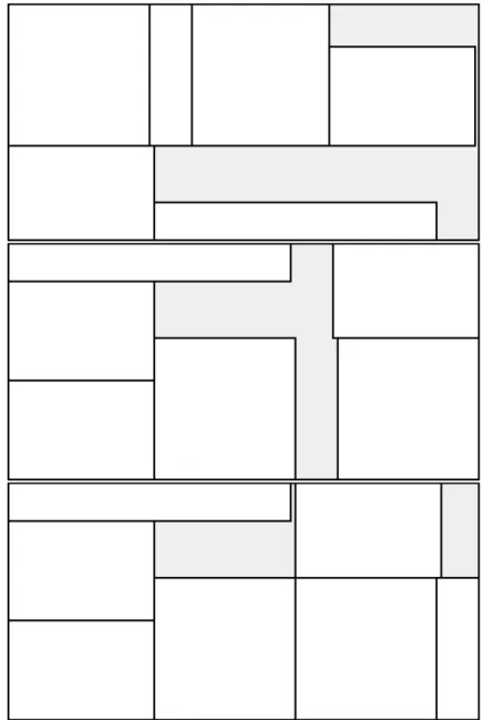
Let us consider an example that shows the differences among the optimal solutions of the Guillotine 2KP obtained by imposing decreasing restrictions to the cuts per-formed.We compare the structure of the optimal solutions for an unweighted instance of two-dimensional knapsack of seven items, where item profits equal their areas. In the left of Figure2.2, we report the optimal solution of the Guillotinetwo-stage 2KP, where the rectangular panel is first divided into horizontal strips, and then items are obtained from the strips by vertical cuts. Further horizontal cuts (trimming) may be necessary to obtain the final items. In the center of the figure, we represent the optimal solution of the Guillotine 2KP when we consider guillotine cuts with anunlimited num-ber of stages, but cuts arerestricted, i.e., they define strips whose width (resp., length) equals the width (resp., length) of some item which is obtained from the strip. The profit of this solution is 9.97% larger than the profit of the two-stage solution. Finally, in the right of the figure we report the optimal solution of the G2KP studied in this chapter: the only restriction imposed to the cuts is to be guillotine ones; they are not restricted nor limited in the number of stages. The profit of this solution, where all the seven items are obtained, is 17.04% larger than the profit of the two-stage solution. The example shows a case where the tree problems have different optimal solutions of strictly increasing profit.
2.1.3 Literature review.
Cutting problems were introduced byGilmore and Gomory[1965], who considered the G2CSP and proposed the k−stage version of the problem. The authors introduced
Figure 2.2: Optimal solutions for an unweighted seven items instance: two-stage 2KP (left), restricted guillotine 2KP (center), guillotine 2KP (right).
the well-known exponential-size model which is usually solved via column generation, where the pricing problem is a one dimensional Knapsack Problem. Since the seminal work of Gilmore and Gomory [1965], a relevant body of literature on two-dimensional cutting has been developed, thus, we mainly concentrate this review on 2KPs, and on guillotine cutting. For a more comprehensive survey on two-dimensional cutting and packing the reader is referred to Lodi et al.[2002] and W¨ascher et al. [2007].
Concerning the 2KP (with no specific restrictions on the cut features),Boschetti et al. [2002] proposed a branch-and-bound algorithm based on a MIP formulation. Caprara and Monaci[2004] andFekete et al.[2007] proposed exact algorithms. The first one is based on a relaxation given by the KP instance with item weights coincident with the
rectangle areas; for this relaxation a worst case performance ratio of 3 is proved. The latter is based on bounding procedures exploiting dual feasible functions.
Restricting the attention to guillotine cutting, the majority of contributions in the recent literature considered the case where the number of stages is limited to two or three. Unless explicitly stated, three stage approaches are for the restricted case. Pisinger and Sigurd [2007] consider the G2CSP and solve the pricing problem as a constraint satisfaction problem, by considering among others the case of guillotine cutting (with limited and unlimited number of stages). Puchinger and Raidl [2007] propose compact models and a branch-and-price algorithm for the three stage G2BPP. They consider the unrestricted case as well. A more application-oriented study is presented in Vanderbeck [2001], where a real-world G2CSP with multiple panel size and additional features is solved via column generation in an approximate fashion. A similar real-world problem, with the additional feature that identical cutting patterns can be processed in parallel, was recently considered by Malaguti et al.[2014].
In terms of optimization models not based on the Gilmore and Gomory (exponential size) formulation, Lodi and Monaci [2003] presented a compact model for the Guil-lotine Two Stage 2KP. Macedo et al. [2010] solved the Guillotine Two Stage 2CSP by extending a MIP formulation proposed by Val´erio de Carvalho [2002] for the one dimensional CSP. The extension of the model to two dimensions asks to define a set of flow problems to determine a set of horizontal strips, and a flow problem to de-termine how the strips fit into the rectangular panel. Silva et al. [2010] presented a pseudo-polynomial size model for the Guillotine Two and Three Stage 2CSP based on the concepts of item to-be-cut and residual plates, obtained after the cut. Recently, Furini and Malaguti[2015] extended this idea to model the Guillotine Two Stage 2KP. Finally, a computational comparison of compact, pseudo-polynomial and exponential size (based on the Gilmore and Gomory formulation) models for the Guillotine Two Stage 2CSP with multiple panel size is presented inFurini and Malaguti [2013]. Few contributions are available in the literature forguillotine cutting problems with an unlimited number of stages. This is probably due to the intrinsic difficulty of model-ing guillotine restrictions. In addition to the mentioned paper by Pisinger and Sigurd [2007], where guillotine restrictions are tackled through constraint satisfaction tech-niques, exact approaches for G2KP have been proposed by Christofides and Whitlock [1977],Christofides and Hadjiconstantinou[1995],Cung et al.[2000]. Cintra and Wak-abayashi [2004] proposed a recursive exact algorithm for the unconstrained case of G2KP, i.e., the case where no upper bound on the number of items of each type ex-ists. A dynamic programming algorithm able to solve large-size instances of the latter problem was recently proposed byRusso et al.[2014]. The most recent exact approach to G2KP is due to Dolatabadi et al. [2012], where a recursive procedure is presented that, given a set of items and a rectangular panel, constructs the set of associated guillotine packings. This procedure is then embedded into two exact algorithms, and
computationally tested on a set of instances from the literature. In addition to the reported exact methods, Hifi [1997] proposed two upper bounding procedures; con-cerning heuristic algorithms, we mention the hybrid algorithm by Hifi [2004] and the recursive algorithm by Chen [2008]. Finally, the related problem of determining if a given set of items can be obtained from a given large rectangle by means of guillotine cuts, was modeled through oriented graphs by Clautiaux et al.[2013].
Despite the relevance of general guillotine cutting problems, the only MIP model in the literature we are aware of was proposed byBen Messaoud et al. [2008], and solves the guillotine GSPP. The model is polynomial in the input size, but in practice it has a very large number of variables and constraints and, as observed in Ben Messaoud et al. [2008], its linear programming relaxation produces “very loose lower bound”. For these reasons the authors report computational experiments where instances with 5 items are solved in non-negligible computing time.
2.1.4 Contribution.
The main contribution of this chapter is to propose a way of modeling general guil-lotine cuts via MIPs. The modeling framework requires a pseudo-polynomial number of variables and constraints, which can be all explicitly enumerated for medium-size instances. To the best of our knowledge, this is the first attempt to model guillotine restrictions via MIPs that works in practice, i.e., once it is implemented within a state-of-the-art solver, can tackle instances of challenging size. In this chapter, we mainly concentrate on the G2KP. We model the problem as a MIP and propose an effective exact method for selecting a subset of the variables containing an optimal solution. Then, the resulting model can be solved by a general purpose MIP solver by only con-sidering the subset of selected variables. This exact procedure is able to significantly increase the number of instances solved to proven optimality. In addition, we propose a number of procedures to further reduce the number of variables and constraints, and discuss conditions under which these reductions preserve the optimality of the solu-tions. We show how the modeling of guillotine cuts can be extended to other relevant problems such as the G2CSP and the GSPP. Finally, we conclude the chapter by an extensive set of computational experiments on benchmark G2KP and GSPP instances from the literature.
2.2
MIP modeling of guillotine cuts
Dyckhoff [1981] proposed a pseudo-polynomial size model for the (one dimensional) Cutting Stock problem, based on the concepts of cut and residual element. The idea is the following: each time a stock of length L is cut in order to produce an item i
to produce additional items. The model associates a decision variable to each item and each (stock or residual) element, and feasible solutions are obtained by imposing balance constraints on the number of residual elements, while the cost of a solution is given by the number of used stock elements.
We extend the approach of Dyckhoff[1981] to two dimensions by using the concepts of cut and plate, where a plate can be either the original rectangular panel or a smaller rectangular residual plate obtained from the panel as result of a sequence of guillotine cuts. We concentrate on the G2KP; the main idea of the model we propose is the following: starting from the initial rectangular panel, we obtain two smaller plates through a horizontal or vertical guillotine cut; for each obtained plate, we need to decide where to perform further cuts, or eventually to keep the plate as it is when its dimensions equal the dimensions of one of the items to obtain. The process is iterated until the plates are large enough to fit some item.
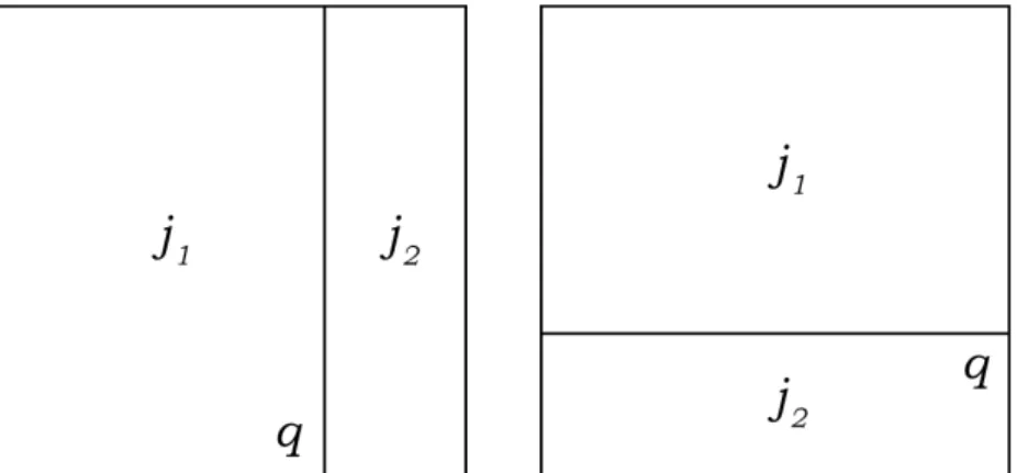
In the model we propose, each cut decision is represented by a triple (q, j, o), where position q denotes the distance from the bottom left corner of a plate j, where a cut with orientation o is performed. In the left of Figure 2.3 we depict a vertical cut performed at position q on a generic plate j, producing two smaller plates j1 and j2. We depict a horizontal cut in the right of the figure.
Figure 2.3: Vertical (left) and horizontal (right) cut at position positionqproducing
two platesj1 andj2.
Without loss of generality we can assume that all problem data are positive integers. We denote by J the set of plates, where the rectangular panel, indexed by j = 0, has dimensions L, W, and each plate j has dimensions (lj, wj), with 1 ≤ wj ≤ W and 1 ≤ lj ≤ L. The actual values of plate dimensions are discussed in the next section. We denote by O = {h, v} the set of possible orientations for a cut (horizontal and vertical, respectively), and by o∈O the generic orientation. We denote by ¯J ⊂J the subset of plates having dimensions equal to one of the items, thus, with a slight abuse of notation, ¯J also denotes the set of items. Without loss of generality, we assume 0∈J¯(in case the rectangular panel does not correspond to an item to obtain, we set
u0= 0). For a platejwe define byQ(j, o) the set of positions where we can cutj with orientation o∈O. We have Q(j, h)⊆ {1, . . . , wj−1} and Q(j, v)⊆ {1, . . . , lj −1).
The model has integer variables xoqj denoting the number of times a plate of typej is cut at position q through a guillotine cut with orientationo. Let aoqkj be a coefficient taking value 1 when a plate of type k is obtained by cutting at position q a plate of type j by a cut with orientation o, and 0 otherwise. In addition, we use the integer variablesyj, j∈J¯, denoting the number of plates of typejthat are kept as final items or, equivalently, the number of items of type j that are obtained.
The G2KP can be modeled as follows
PP−G2KP : maxX j∈J¯ pjyj (2.1) X k∈J X o∈O X q∈Q(k,o) aoqkjxoqk− X o∈O X q∈Q(j,o) xoqj −yj ≥0 j∈J , j¯ 6= 0 (2.2) X k∈J X o∈O X q∈Q(k,o) aoqkjxoqk− X o∈O X q∈Q(j,o) xoqj ≥0 j ∈J\J¯ (2.3) X o∈O X q∈Q(0,o) xoq0+y0≤1 (2.4) yj ≤uj j ∈J¯ (2.5) xoqj ≥0integer j∈J, o∈O, q∈Q(j, o) (2.6) yj ≥0 integer j∈J ,¯ (2.7)
where the objective function (2.1) maximizes the profit of cut items; constraints (2.2) impose that the number of plates j that are cut or kept as items does not exceed the number of platesjobtained through the cut of some other plates; constraints (2.3) are equivalent to the previous constraints for plates j /∈ J¯(hence, the corresponding yj variables are not defined); constraint (2.4) impose that the original rectangular panel is not used more than once; constraints (2.5) impose not to exceed the maximum number of items which can be obtained. Finally, (2.6) and (2.7) force the variables to be non-negative integers.
The model has a pseudo-polynomial size, indeed, in the worst case the number of plates is W L, and each plate can be horizontally cut inO(W) positions and vertically cut in
O(L) positions. The overall number ofxvariables is thusO(W L(W+L)), in addition to the y variables of which there are n. In the following, we denote this pseudo-polynomial size model as PP-G2KP Model. Indeed, not all the plates (accordingly, the variables and the constraints of the PP-G2KP Model) are necessary to preserve
the optimality of the solutions. In the following, we discuss different ways of safely reducing the number of variables and constrains for the PP-G2KP Model.
The plates and, accordingly, the model variables can be enumerated by processing the item set ¯J and the rectangular panel (plate 0) as described in Procedure 1. Starting from plate 0, new plates are obtained through vertical and horizontal cuts (line 7), and stored in set J when their size is such that they can fit some item (lines 9-12); otherwise the new plate is discarded. The definition of the set of positions Q(j, o) where plate j is cut with orientationo(line 5) is discussed in the next section.
Algorithm 1:Plate-and-variable enumeration
Require: plate 0, items set ¯J Ensure: plates setJ, variablesx
1: initializeJ={0}, mark 0 as non-processed; 2: whileJcontains non-processed platesdo
3: select a non-processedj∈J; 4: for allo∈ {h, v}do
5: compute the set of cut positionsQ(j, o); 6: for allpositionsq∈Q(j, o)do
7: cutjatqwith orientationo, generate platesj1,j2; 8: if j1 6∈Jandj1 can fit some item then
9: setJ=J∪ {j1}; 10: end if
11: if j2 6∈Jandj2 can fit some item then 12: setJ=J∪ {j2}; 13: end if 14: createxoqj; 15: end for 16: end for 17: markjas processed; 18: end while 19: return J,x.
A related extension of the model in Dyckhoff [1981] was proposed by Silva et al. [2010] to model two and three stage restricted guillotine 2CSPs. InSilva et al.[2010], a decision variable defines the cut of an item from a plate through two orthogonal guillotine cuts, which in addition to the item produce (up to) two residual plates. This idea cannot be extended to the unrestricted case, where the position of a cut may not correspond to the size of an item. In the following section we provide a lower bound on the largest profit loss which is incurred by considering the restricted case instead of the unrestricted one. An extension of the model of Silva et al. [2010] to two stage guillotine knapsack problems is discussed in Furini and Malaguti[2015].
Finally, we mention Arbib et al. [2002], where a further extension of the model in Dyckhoff [1981] is presented. The authors consider a one dimensional Cutting Stock problem where the residual elements can be re-used and, in the specific application case, combined, so as to obtain the requested items.
2.2.1 Definition of the cut position set
Model (2.1)–(2.7) can have very large size, depending on the cardinality of sets J and
Q(j, o),j ∈J,o∈O. The number of plates that we consider and the number of cuts performed on each plate (eventually producing new plates) determine, in practice, the size of the model. Thus, a crucial question to be answered is the following:
Given a plate j of length lj and width wj, how should Q(j, o), o ∈ O, be defined in order to minimize the number of variables and plates of the model, while preserving the optimality of the solution?
LetIj be the set of items that can fit into platej, i.e.,Ij ={i∈J¯: li ≤lj, wi≤wj}. The complete position set (Q) where a cut can be performed includes the dimensions of items i∈Ij, and all combinations of the items i∈Ij dimensions, and is defined as follows: Q(j, h) = q : 0< q < wj; ∀i∈Ij, ∃ni ∈N, ni ≤ui, q= X i∈Ij niwi , (2.8) and Q(j, v) = q: 0< q < lj; ∀i∈Ij, ∃ni∈N, ni ≤ui, q= X i∈Ij nili . (2.9)
These positions are known in the literature as discretization points, and a pattern where cuts are performed at discretization points is known as a normal or canonical pattern, see Christofides and Whitlock [1977], Herz [1972]. All the combinations of items defining the complete position set can be effectively obtained by a Dynamic Programming (DP) algorithm. The DP algorithm we used is an extension to the case of items available in several copies of the one described in Trick [2003] (which only considers single items).
Let us also define the restricted position set (QR), including only the dimensions of items i∈Ij, as:
QR(j, h) ={q : ∃i∈Ij, q=wi}, QR(j, v) ={q: ∃i∈Ij, q=li}. (2.10)
Note that one can remove symmetric cut positions for a platej from setQ(j, o), o∈O
(resp. QR(j, o)), i.e.:
(wj−q)∈/ Q(j, h), ∀q∈Q(j, h), q < wj/2 (lj−q)∈/ Q(j, v), ∀q ∈Q(j, v), q < lj/2.
Considering thePP-G2KP Model with the restricted position set only, does not guar-antee in general the optimality of the corresponding solution. The following theorem states a condition under which the optimality is preserved.
Theorem 2.1. If a plate j can fit at most five items by guillotine cuts, then an opti-mal solution to the PP-G2KP Model exists by considering the positions q for plate j
restricted to QR(j, h) and QR(j, v).
Proof. Proof of Theorem 2.1. We need to show that, when cutting five items from a plate, any packing can be obtained by considering restricted cut positions only. With-out loss of generality, consider the first cut to be vertical. When performing the first guillotine cut, either we obtain two new plates which contain two and three items, re-spectively; or we obtain two new plates which contain one and four items, respectively. In the latter case the first cut can be performed at a position corresponding to the length of the item which is alone in the new plate. Assume instead the first case holds, and consider the new plate containing two items. If they are placed one on the side of the other (as in the left of Figure2.4), it was possible to separate one of them with the first cut. When the two items are placed one on top of the other (as in the right of Figure 2.4), the first cut could be performed at a position equal to the length of the longest of the two. Similar considerations apply when cutting four items from a plate.
Figure 2.4: Possible configurations after separating five items with a vertical
guil-lotine cut.
Consider the following
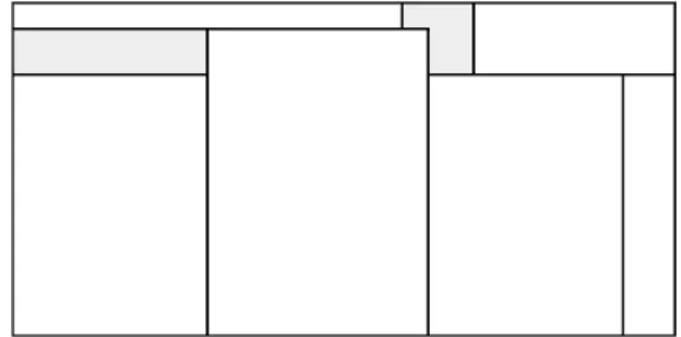
Example 1. Consider an instance of the G2KP of six items with dimensions l = [47,40,40,40,11,4] andw= [34,30,30,8,31,60] and a rectangular panel of dimensions
L = 102, W = 51 (see Figure 2.5). All items can be obtained from the rectangular panel through guillotine cuts (in Figure 2.5, the first cut is vertical and separates the panel in two new plates containing three items each), but no feasible solution to the PP-G2KP Model with q restricted to QR(j, o), o∈O allows to obtain the six items.
From Example1 it follows that
Figure 2.5: A six items packing that cannot be obtained by considering restricted positionsQRonly.
Given the result of Theorem 2.1, a reduction in the number of variables of the PP-G2KP Model can be obtained by considering positions in set QR for plates with the property that they can fit at most five items. Since exactly checking this condition can be computationally expensive, we considered the following relaxation. A sufficient condition for this property to hold is that the cumulate area of the six smallest items exceeds the plate area. In the following we denote the reduction obtained by checking the previous sufficient condition as Cut-Position reduction.
Restricting the positions to QR(j, h) and QR(j, v) for all plates has a large impact on the number of variables and plates of the PP-G2KP Model (see Section2.4.1) but potentially leads to sub-optimal solutions. Thus it is natural to wonder what is the loss of profit in the worst case. In the following we denote the PP-G2KP Model with variables restricted to the the position setsQR asRestricted PP-G2KP model. LetzR be the optimal solution of theRestricted PP-G2KP model, andzU the optimal solution of the PP-G2KP Model (with complete position and Q). The following proposition provides an upper bound on the profit in the worst case.
Remark 2.3. In the worst case, zR zU ≤
5 6.
Proof. Proof of Remark2.3. The result follows from Example1when the profit is the same for all the six items.
Notice that theRestricted PP-G2KP model allows to perform a cut on a plate without obtaining a final item: this may happen each time the dimension of an item is the combination of the dimensions of two or more smaller items. As an example, if there are three items with widths 2,3,5, theRestricted PP-G2KP model would allow to cut at positionq = 5, and then to perform a further cut at positionq = 2 on the obtained plate. Hence, the width of the strip obtained by cutting at position 5 would not correspond to the width of one of the obtained items. For this reason, the Restricted PP-G2KP model can produce solution which do not satisfy the definition of restricted guillotine cuts given in Section 2.1.
In order to solve the restricted G2KP, one possibility is to extend the modeling ideas presented by Silva et al. [2010] for the Guillotine Two and Three Stage 2CSP, and adapted by Furini and Malaguti [2015] to the 2KP. By removing the limitation on the number of stages, the model in Furini and Malaguti[2015], which cuts items from plates, can solve the restricted G2KP.
Another reduction of the model size can be obtained by removing redundant cuts (de-noted asRedundant-Cutreduction in the following). Note that, while theCut-Position
reduction can reduce the number of plates in the model, theRedundant-Cutreduction do not affect the number of plates, but only the number of cut positions (and thus the variables of the model).
We say that q is a trim cut on plate j when cutting platej at position q produces a single useful plate j1 (the second produced plate j2 is waste).
Remark 2.4. Given a platej, one can remove a trim cut at positionq with orientation
ofromQ(j, o), while preserving the optimality of the solution of thePP-G2KP Model, in the following cases:
1. Plate j canonly be obtained through a sequence of two orthogonal trim cuts on a larger plate.
2. Plate jcan be obtained from one or more larger plates, but always through trim cuts, and at least one of these trim cuts has orientation o.
Proof. Proof of Remark 2.4. In both cases, plate j is obtained anyway through an alternative cut sequence, and thus the corresponding variable can be removed from the model preserving optimality.
Figure 2.7: Trim cuts on plate 1 producing item 2b can be removed.
As an example of the first case, consider top of Figure2.6: plate 0 is vertically trimmed obtaining plate 1, and plate 1 is horizontally trimmed obtaining plate 2. There are no other plates that can be cut to produce plate 2. The further trim cut of plate 2 to obtain plate 3 can be safely removed, because plate 3 is also obtained in the sequence 0→4→3.
As an example of the second case, consider plate 1 in Figure 2.7. Since plate 1 is simultaneously generated from 0 and from 3 through a vertical and horizontal trim cut, respectively, no further trim cuts are considered on plate 1.
Conditions 1 and 2 of Remark 2.4 are checked during the enumeration of plates and variables through Procedure 1. In order to check these conditions, we associate four flags to each plate. The flags can assume values -1, 0, 1 (obtained only through a trim cut, not obtained through a cut with the same orientation, obtained without a trim cut):
• Flagshindicates the status of the plate with respect to a cut with orientationh;
• Flagsvindicates the status of the plate with respect to a cut with orientationv;
• Flagf h indicates the status of flags shfor all the father plates of the plate;
At step 3 of Procedure 1 we select platej, and check if it can be eventually obtained by further cuts from plates inJ. If this is the case, we cannot safely remove redundant cuts, otherwise, at step 6:
• if one (or more) of the flags of platej has value -1, do not perform trim cuts on
j in the flag orientation.
At step 7, if anew plate j1∈/ J is obtained fromj through a trim cut with orientation
h:
• set the flag shof j1 to -1;
• set the flag sv ofj1 to 0;
• set the flagsf h and f v equal to flagssh and svof j;
if a new plate j1 is obtained fromj through a trim cut with orientation v:
• set the flag sv ofj1 to -1;
• set the flag shof j1 to 0;
• set the flagsf h and f v equal to flagssh and svof j;
if an existing plate j1∈J is obtained fromj through a trim cut:
• ifsh ofj is larger than -1, set the flagf h ofj1 to 1;
• ifsv of j is larger than -1, set the flagf v ofj1 to 1;
if a plate (new or existing) j1 is obtained from j without a trim cut:
• set all flags of j1 to 1.
The computational effect on the number of variables and plates of the reductions discussed in this section are highlighted in Section 2.4.
2.2.2 Model extensions: Cutting Stock problem and Strip Packing problem
The modeling ideas of Section 2.2 can be extended to model other two-dimensional guillotine cutting problems. We present in this section two MIP models for the G2CSP and the GSPP.
By using the same variables defined for the PP-G2KP Model, a MIP formulation for the G2CSP reads as follows
PP−G2CSP : min X o∈O X q∈Q(0,o) xoq0+y0 (2.11) (2.2),(2.3) yj ≥dj j ∈J ,¯ (2.12) xoqj ≥0 integer j∈J, o∈O, q∈Q(j, o) (2.13) yj ≥0integer j∈J¯ (2.14)
where the objective function (2.11) minimizes the number of rectangular panels that are used; and constraints (2.12) impose to satisfy the demand associated with the items. The remaining constraints have the same meaning as in the PP-G2KP Model. The PP-G2CSP model can be extended to the case of panels available in p different sizes, by defining p initial panels 0t and a coefficient ct, t = 1, . . . , p, specifying the corresponding cost. The objective function is promptly modified to:
min X t=1,...,p ct( X o∈O X q∈Q(0t,o) xoq0t+y0t). (2.15)
To model the GSPP, we first need an upper bound W on the optimal solution value. We consider the first cut performed on the strip (j = 0) to be horizontal (h), with
Q(0, h) ={1, . . . , W} and do not define vertical cuts for the strip (i.e.,Q(0, v) ={∅}); in addition, out of the two parts obtained from the first cut, only the bottom one is a finite rectangle that can be used, while the top part is the residual of the infinite strip. The width of the obtained initial rectangle is in Q(0, h) and equals the solution value. We use a variable z denoting the solution value, in addition to the variables defined for the PP-G2KP Model. A MIP formulation for the GSPP is then
PP−GSPP : min z (2.16) z≥qxhq0 q ∈Q(0, h) (2.17) X q∈Q(0,h) xhq0= 1 (2.18) (2.2),(2.3) yj ≥dj j∈J¯ (2.19) xoqj ≥0 integer j∈J, o∈O, q∈Q(j, o) (2.20) yj ≥0integer j∈J¯ (2.21)
where the objective function (2.16) and constraints (2.17) minimize the (vertical) dis-tance of the first cut from the bottom of the strip, constraint (2.18) impose to have one horizontal first cut (whereq is the width of the cut, withq ∈Q(0, h)). The remaining constraints have the same meaning as in the previous models.
2.3
An effective solution procedure for the
PP-G2KP
Model
Tackling directly the PP-G2KP Model through a general-purpose MIP solver can be out of reach for medium-size instances due to the large number of variables and con-straints, thus in this section we describe an effective exact solution procedure based on variable pricing, aiming at reducing the number of variables and quicken the compu-tational convergence.
The procedure starts by enumerating all the PP-G2KP Model variables by means of Algorithm 1, considering the complete position set Q (see Section 2.2). Symmetric cut positions are not generated (Section2.2.1). Variables are then stored in avariable pool. We denote the PP-G2KP Model with all these variables asComplete PP-G2KP Model. The variable pool of the Complete PP-G2KP Model can be preprocessed by means of the Cut-Position and Redundant-Cutreductions, so as to reduce its size. We perform two subsequent variable pricing procedures executed in cascade. The first one concerns the solution of the linear relaxation of the PP-G2KP Model, where variables having positive reduced profit are iteratively selected from the variable pool. The value of the linear programming relaxation of the PP-G2KP Model, denoted as
LP in the following, gives an upper bound on the optimal integer solution value. By exploiting the dual information from the linear programming relaxation, and by computing a feasible solution of value LB, a second pricing of the variables can be performed. This second variable pricing allows us to select from the variable pool all the variables that, by entering in the optimal base with an integer value (e.g., after a branching decision), could potentially improve on the incumbent solution of value LB. We denote thePP-G2KP Model after the second variables pricing asPriced PP-G2KP Model.
The details on the two variable pricing procedures are given in the next section.
2.3.1 Variable pricing procedures
The linear programming relaxation of the PP-G2KP Model can be solved by variable pricing, where we iteratively solve the model with a subset of variables and exploit
dual information to add variables with positive reduced profit. Initially, we relax the integrality requirements for the variables (constraints (2.6) and (2.7)) to:
xoqj ≥0 j∈J, o ∈O, q∈Q(j, o), (2.22)
yj ≥0 j∈J ,¯ (2.23)
and we initialize the resulting linear program (2.1)–(2.5) and (2.22), (2.23) with all the yj, j ∈ J¯ variables and the xqjo , j ∈ J, o ∈ O, q ∈ QR(j, o) variables, i.e., variables corresponding to cuts in the restricted positions set QR (see Section 2.2). The solution of the resulting linear programming relaxation provides optimal dual variables πj associated with constraints (2.2) and (2.3).
The reduced profit of a variable xoqj, associated with a cut of platej producing (up to) two new plates j1 andj2, is readily computed as:
˜
p(xoqj) =πj1 +πj2−πj, (2.24)
and can be evaluated for all the variables of the Complete PP-G2KP Model, stored in the pool, in linear time in the size of the pool. The reduced profit ˜p(xoqj) repre-sents the change in the objective function for an unitary increase in the value of the corresponding variable xoqj.
We optimally solve the linear relaxation of the PP-G2KP Model by iteratively adding variables with positive reduced profit, i.e., a subset of
xoqj, j ∈J, o∈O, q∈Q(j, o) : ˜p(xoqj)>0 ,
and then re-optimizing the corresponding linear program. When all variables in the variable pool have a non-positive reduced profit, then the linear programming relax-ation of the Complete PP-G2KP Model is optimally solved, providing us an upper bound of value LP.
Given a feasible solution of valueLB, the optimal valueLP of the linear programming relaxation, and the optimal value of the dual variables πj∗, j ∈ J, we perform a last round of pricing. ThePriced PP-G2KP Model is defined by including they variables and the subset of thex variables
xoqj, j ∈J, o∈O, q∈Q(j, o) :bp˜(xoqj) +LPc> LB .
This includes all the variables in base plus the variables that, by entering in the current basic solution with value 1 (i.e., at the minimal non-zero integer value), would produce a solution of value z > LB.
The effectiveness of the last round of variable pricing in reducing the number of vari-ables of the Priced PP-G2KP Model largely depends on the gap between the upper
bound valueLP and the value of a feasible solutionLB. Heuristic feasible solutions of excellent quality can be computed by solving theRestricted PP-G2KP model, defined by the variables from the restricted position setQr (see Section2.4.1in the following).
The exact solution procedure is summarized in Algorithm2.
Algorithm 2:Solution procedure for the PP-G2KP Model
1: SetLBto the value of a feasible solution to thePP-G2KP Model; 2: Generate the variable pool through Algorithm1;
3: Apply theCut-PositionandRedundant-Cutreductions to the pool variables; 4: Initialize the model with the variables of the restricted position setQR; 5: repeat
6: Solve the linear programming relaxation, compute reduced profits, add the variables with positive reduced profit from the pool,
7: untilvariables with positive reduced profit exist;
8: LetLP be the optimal solution value of the linear relaxation of thePP-G2KP Model; 9: Final Pricing: define thePriced PP-G2KP Model by including thexvariables with reduced
profit ˜p(x) such thatbp˜(x) +LPc> LB, and all theyvariables; 10: Solve thePriced PP-G2KP Model with a MIP solver.
2.4
Computational Experiments
To the best of our knowledge, the modeling framework of guillotine restrictions that we propose in this chapter is the first approach based on Mixed-Integer Linear Pro-gramming that is able to solve benchmark instances to optimality. Thus, the scope of the reported computational experiments is broader than simply comparing the ob-tained results against previous approaches. Namely, with these experiments we wish to evaluate:
• the size and practical solvability of the Complete PP-G2KP Model for a set of G2KP benchmark instances by means of a general purpose MIP solver;
• the effectiveness of the proposed Cut-Position and Redundant-Cut reductions in removing variables and constraints from theComplete PP-G2KP Model . • the capability to solve the PP-G2KP Model by means of the pricing procedure
described in Section 2.3(Priced PP-G2KP Model);
• the quality of the solutions that are obtained by optimally solving thePP-G2KP Model by considering the restricted position setQR only;
• finally, we wish to discuss the computational performance of our framework with respect to a state-of-the-art combinatorial algorithm for the G2KP (Dolatabadi et al.[2012]), and with the only alternative MIP formulation of guillotine restric-tions we are aware of, which is described for the GSPP (Ben Messaoud et al. [2008]).
We performed all the computational experiments on one core of a Core2 Quad Q9300 2.50GHz computer with 8 GB RAM, under Linux operating system. As linear pro-gramming and MIP solver we used IBM ILOG CPLEX 12.5.
In the computational experiments, we considered two sets of classical two-dimensional instances, listed in Table2.1. The first set of 21 instances, for whichDolatabadi et al. [2012] reports computational results as well, is from the OR library (OR-Library); the second set of 38 instances is fromHifi and Roucairol[2001]. Both sets include weighted and unweighted instances, where the profit of each item is given, or equals the item area, respectively.
unweighted weighted
OR-Library gcut1 - gcut12, wang20, cgcut1 - cgcut3, okp1 - okp5, 2s, 3s, A1s , A2s, STS2s, HH, 2, 3, A1, A2, STS2,
Hifi and Roucairol[2001] STS4s, OF1, OF2, W, CHL1s, STS4, CHL1, CHL2, CW1, CHL2s, A3, A4, A5, CHL5, CW2, CW3, Hchl2, Hchl9. CHL6, CHL7, CU1, CU2,
Hchl3s, Hchl4s, Hchl6s, Hchl7s, Hchl8s.
Table 2.1: List of the considered G2KP instances.
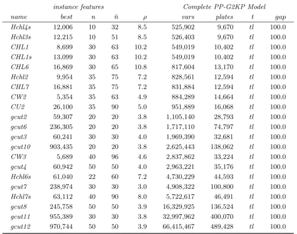
In order to classify the instances according to the size, we generated the Complete PP-G2KP Model, and we grouped the instances into three sets, according to the cor-responding number of variables. Table 2.2, 2.3 and 2.4 reports the features of small (less than 100,000 variables), medium (between 100,000 and 500,000 variables), and large-size instances, having more than 200,000 variables).
For each instance, the table reports the name (name), the optimal solution value (opt), the number of different itemsn, the total number of items ¯n, the largest ratio between an item length or width and the length or width of the rectangular panel (ρ). Then the table reports the number of variables of theComplete PP-G2KP Model (vars) and the corresponding number of plates (plates). We solved the model with the CPLEX MIP solver by allowing 1 hour of computing time. The table reports the effective computing time (t) and the corresponding percentage optimality gap (gap), computed as 100(U BM IP−LBM IP)
U BM IP (where U BM IP and LBM IP are the lower and upper bound achieved by the MIP solver at the end of the computation).
The size of theComplete PP-G2KP Model can be very large, in particular for the gcut
instances, the largest model (gcut12) has more than 66 million variables and almost 0.5 million constraints. In addition to a very large size, since no reductions are applied to theComplete PP-G2KP Model, it may contain equivalent solutions. The CPLEX MIP solver can solve to optimality 24 out of 26 small-size instances, 12 out of 18 medium-size instances, and none of the 21 large-medium-size instances. For instance A5 and all the
instance features Complete PP-G2KP Model
name best n n¯ ρ vars plates t gap
cgcut1 244 7 16 10.0 801 140 0.1 0.0 CHL5 390 10 18 20.0 2,858 345 0.6 0.0 Hchl8s 911 10 18 49.0 13,997 896 tl 1.8 OF2 2,690 10 24 10.0 37,261 2,110 66.0 0.0 cgcut3 1,860 19 62 6.4 38,485 1,860 58.6 0.0 wang20 2,721 19 42 6.4 38,485 1,860 60.7 0.0 3 1,860 20 62 6.4 38,485 1,860 81.6 0.0 3s 2,721 20 62 6.4 38,485 1,860 60.7 0.0 W 2,721 20 62 6.4 38,485 1,860 56.5 0.0 OF1 2,737 10 23 10.0 38,608 2,098 53.9 0.0 gcut1 48,368 10 10 3.8 39,896 4,429 8.8 0.0 A1 2,020 20 62 5.6 45,333 2,040 85.4 0.0 A1s 2,950 20 62 5.6 45,333 2,040 82.3 0.0 cgcut2 2,892 10 23 10.0 52,590 2,017 58.4 0.0 2 2,892 10 23 10.0 52,590 2,017 55.2 0.0 2s 2,778 10 23 10.0 52,590 2,017 57.2 0.0 CHL2 2,326 10 19 6.1 57,567 2,348 104.1 0.0 CHL2s 3,279 10 19 6.1 57,567 2,348 110.4 0.0 A2 2,505 20 53 5.0 61,047 2,276 236.6 0.0 A2s 3,535 20 53 5.0 61,047 2,276 131.0 0.0
Table 2.2: Small-size instances.
instance features Complete PP-G2KP Model
name opt n ¯n ρ vars plates t gap
STS2 4,620 30 78 8.5 118,036 3,383 289.8 0.0 STS2s 4,653 30 78 8.5 118,036 3,383 385.7 0.0 Hchl9 5,240 35 76 7.6 130,738 3,666 612.5 0.0 A3 5,451 20 46 5.7 134,164 3,752 435.5 0.0 HH 11,586 5 18 7.5 141,167 5,486 tl 4.5 A4 6,179 20 35 10.0 179,759 4,860 1,259.0 0.0 gcut5 195,582 10 10 3.8 250,327 25,336 tl 1.4 okp1 27,589 15 50 100.0 255,497 7,947 490.5 0.0 okp3 24,019 30 30 33.3 261,074 8,356 tl 8.8 okp4 32,893 33 61 100.0 287,773 9,049 684.4 0.0 okp2 22,503 30 30 100.0 289,825 9,506 tl 30.0 CU1 12,330 25 82 5.0 335,415 7,700 1,460.8 0.0 STS4 9,700 20 50 7.1 352,590 7,224 2,476.6 0.0 STS4s 9,770 20 50 7.1 352,590 7,224 2,452.4 0.0 okp5 27,923 29 97 100.0 368,529 9,506 2,118.6 0.0 CW1 6,402 25 67 5.0 410,004 8,407 tl 70.7 gcut9 919,476 10 10 3.4 474,360 38,936 2,847.9 0.0 A5 12,985 20 45 10.2 494,455 10,402 tl 100.0
Table 2.3: Medium-size instances.
larger ones, gaps at time limit are 100%, meaning that no feasible solution is found by the solver.
instance features Complete PP-G2KP Model
name best n n¯ ρ vars plates t gap
Hchl4s 12,006 10 32 8.5 525,902 9,670 tl 100.0 Hchl3s 12,215 10 51 8.5 526,403 9,670 tl 100.0 CHL1 8,699 30 63 10.2 549,019 10,402 tl 100.0 CHL1s 13,099 30 63 10.2 549,019 10,402 tl 100.0 CHL6 16,869 30 65 10.8 817,604 13,170 tl 100.0 Hchl2 9,954 35 75 7.2 828,561 12,594 tl 100.0 CHL7 16,881 35 75 7.2 831,884 12,594 tl 100.0 CW2 5,354 35 63 4.9 884,289 14,664 tl 100.0 CU2 26,100 35 90 5.0 951,889 16,068 tl 100.0 gcut2 59,307 20 20 3.8 1,105,140 28,793 tl 100.0 gcut6 236,305 20 20 3.8 1,717,110 74,797 tl 100.0 gcut3 60,241 30 30 4.0 1,969,390 32,681 tl 100.0 gcut10 903,435 20 20 3.8 2,625,443 138,062 tl 100.0 CW3 5,689 40 96 4.6 2,837,862 33,224 tl 100.0 gcut4 60,942 50 50 4.0 2,963,221 35,176 tl 100.0 Hchl6s 61,040 22 60 7.2 4,730,229 44,593 tl 100.0 gcut7 238,974 30 30 3.0 4,908,322 100,800 tl 100.0 Hchl7s 63,112 40 90 8.0 5,722,617 46,491 tl 100.0 gcut8 245,758 50 50 3.9 16,329,925 136,524 tl 100.0 gcut11 955,389 30 30 3.8 32,997,962 400,070 tl 100.0 gcut12 970,744 50 50 3.9 66,415,467 489,428 tl 100.0
Table 2.4: Large-size instances.
2.4.1 Lower bound (feasible solution) computation
Computing a feasible solution is the first step of the solution procedure for the PP-G2KP Model, summarized in Algorithm2. A possible fast way of computing a feasible solution is by the iterated greedy algorithm proposed byDolatabadi et al.[2012]: given a random order of the items, the algorithm selects the firstkitems in the ordering whose cumulate profit would improve on the incumbent solution. The algorithm then tries to pack the selected items into the rectangular panel, according to a First Fit Decreasing strategy (see Coffman et al. [1980]); in case of success, the incumbent solution is updated (the attempt is not performed if the sum of the areas of the selected items is larger than the area of the panel). In our implementation, we allow 1 million of iterations after the last update of the incumbent solution.
Improved feasible solutions can be obtained by considering the optimal solution of the PP-G2KP Model with cut positions in the restricted position set QR, i.e., the Restricted PP-G2KP model. Example 1 tells us that the Restricted PP-G2KP model might not contain the optimal solution. However, this occurrence is rare in practice and, in any case, the optimal solution value of the Restricted PP-G2KP model is a valid lower bound LB on the optimal solution value.
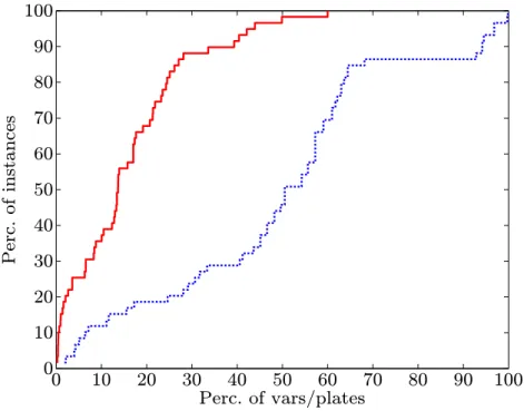
In order to show the relative size of theRestricted PP-G2KP model, in Figure2.8we use performance profiles to depict the percentage of variables and plates of the Restricted PP-G2KP model with respect to variables and plates of theComplete PP-G2KP Model. In the horizontal axis the figure reports the percentage of variables (resp., plates), and in the vertical axis the percentage of instances for which the Restricted PP-G2KP model has no more than the corresponding percentage of variables (resp., plates). The continuous line is for the variables, the dashed line for the plates. We see that for 80% of the instances, the Restricted PP-G2KP model has at most 25% of the variables and 65% of the plates of the Complete PP-G2KP Model.
0 10 20 30 40 50 60 70 80 90 100 0 10 20 30 40 50 60 70 80 90 100 Perc. of vars/plates P er c. o f in st a n ce s
Figure 2.8: Variables and plates of theRestricted PP-G2KP model with respect to
theComplete PP-G2KP Model.
Despite the large reduction in the number of variables and plates, solving theRestricted PP-G2KP model by using a MIP solver can be very time consuming, hence, we adapted the pricing procedure of Algorithm 2 to this case. We compute an initial feasible solution by means of the iterated greedy algorithm, we solve the linear programming relaxation of the Restricted PP-G2KP model, and we price the model variables, thus defining a Restricted Priced PP-G2KP Model containing only the variables that, by entering in base with value 1 or larger, could improve on the incumbent solution. Then, we solve the resultingRestricted Priced PP-G2KP Modelby means of the CPLEX MIP solver.
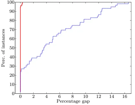
In Figure 2.9 we use performance profiles to represent the gaps between the values of the greedy heuristic solution (LBg) and of the Restricted PP-G2KP model (LBR) optimal solution, and the value of the best solution we can compute. In the horizontal axis of the figure we report the percentage gap, computed as 100(best−LB)/best,