Direct numerical simulation of a wall jet: flow physics

Direct numerical simulation of a wall jet:

Flow physics

Iftekhar Z. Naqavi

†

, James C. Tyacke and Paul G. Tucker

(Received xx; revised xx; accepted xx)

A direct numerical simulation (DNS) of a plane wall jet is performed at a Reynolds number ofRej = 7500. The streamwise length of the domain is long enough to achieve self-similarity for the mean flow and the Reynolds shear stress. This is the highest Reynolds number wall jet DNS for a large domain achieved to date. The high resolution simulation reveals the unsteady flow field in great detail and shows the transition process in the outer shear layer and inner boundary layer. Mean flow parameters of maximum velocity decay, wall shear stress, friction coefficient and jet spreading rate are consistent with several other studies reported in the literature. Mean flow, Reynolds normal and shear stress profiles are presented with various scalings, which reveals the self-similar behaviour of the wall jet. The Reynolds normal stresses do not show complete similarity for the given Reynolds number and domain length. Previously published inner layer budgets based on LES are inaccurate and those that have been measured are only available in the outer layer. The current DNS provides fully balanced, explicitly calculated budgets for the turbulence kinetic energy, Reynolds normal stresses and Reynolds shear stress in both the inner and outer layers. The budgets are scaled with inner and outer variables. The inner scaled budgets in the near wall region show great similarity with turbulent boundary layers. The only remarkable difference is for the turbulent diffusion in the wall-normal Reynolds stress and Reynolds shear stress budgets . The outer layer interacts with the inner layer through turbulent diffusion and the excess energy from the wall normal direction is transferred to the spanwise direction.

Key words: Authors should not enter keywords on the manuscript, as these must

be chosen by the author during the online submission process and will then be added during the typesetting process (see http://journals.cambridge.org/data/relatedlink/jfm-keywords.pdf for the full list)

1. Introduction

Launder & Rodi (1983) defined a wall jet as ‘a boundary layer in which, by virtue of the initially supplied momentum, the velocity over some region in the shear layer exceeds that in the free stream’. Normally, for a wall jet, fluid exits from a slot at high velocity and flows along a wall. Wall jets are characterised by the presence and interaction of two shear layers. The first is from the boundary layer, developing due to the high momentum fluid along the wall, also called the ‘inner layer’. The second develops between the high momentum fluid of the jet and the outer ambient conditions, which can be quiescent, or moving with a different speed than the jet and is called the ‘outer layer’. The two

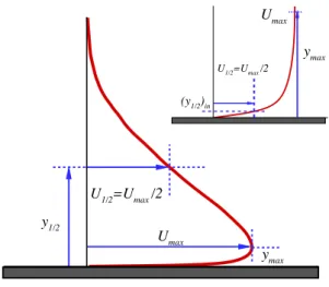
y_max Umax y_1/2 U1/2=Umax /2 ymax Umax (y1/2)in U1/2=Umax /2

Figure 1: Various length and velocity parameters used for wall jet scaling.

layers have different kinds of large scale structures responsible for the generation of shear strain, which produce turbulence. These structures interact with each other. The inlet wall jet Reynolds number can be defined asRej=

Ujh

ν , where his the slot height,Uj is the jet slot exit velocity andν is the kinematic viscosity. The mean streamwise velocity profile of a turbulent wall jet in the fully developed region is shown in Figure 1. This profile is characterised by a maximum velocity Umax, which separates the two layers in this flow. The location of the maximum velocity is designated asymax. A length scale for the outer layer is defined asy1/2. This is the wall normal distance aboveymax, where the streamwise velocity is half of the maximum velocity i.e. 1₂Umax. A similar length scale (y1/2)incan be defined for the inner layer, which is the wall normal distance belowymax, where the streamwise velocity again becomes 1

2Umax.

Wall jets find wide ranging application in separation control on airfoils (Dunham 1968), and in the film-cooling of combustion chamber liners and leading stage blades in gas turbines (Launder & Rodi 1983). In the case of separation control, the objective is to achieve enhanced near wall momentum and increased mixing between the wall jet and the outer flow to suppress separation. On the other hand, for film-cooling applications, the jet and ambient flow should have minimum mixing. These are opposite requirements and for efficient application, a greater understanding of this flow is needed at more relevant Reynolds numbers.

Since Glauert (1956), who coined the term wall jet and made the first attempt to achieve a boundary layer solution for this, several analytical, experimental and numerical studies have been performed. Launder & Rodi (1983) gave a comprehensive overview of pre-1980 wall jet research. More recently Banyassady & Piomelli (2014) reviewed the latest work on wall jets. A significant amount of work is concerned with the self-similar solution or behaviour of the wall jet. Georgeet al.(2000) explained the significant benefits in defining self-similarity as follows: ‘Only a similarity solution provides an unambiguous test of a turbulence model independent of computational constraints and experimental difficulties. It does not depend on computational grid, domain, or differencing schemes, nor does it depend on difficulties in realising and measuring a laboratory flow. It exists independent of closure approximations, and thus the scaling laws it offers can be used to

test closure hypotheses. Its straightforward boundary conditions are free from the finite limits of experimental facilities or computer memories, and thus its profiles provide an ideal reference for testing the effects of enclosure.’

A similarity solution was obtained by dividing the wall jet into inner and outer layers (Glauert 1956; Schwarz & Cosart 1961; Myerset al.1963). The inner layer is considered similar to the boundary layer, with Umax as the free stream velocity and ymax acting as the boundary layer thickness. The outer layer aboveymax is treated as half of a free jet. This is a remarkably simple picture, however it is not supported by measurements. The inner layer does not follow the turbulent boundary layer behaviour exactly and is influenced by the outer layer turbulence. Also, the outer layer does not expand like a free jet due to the presence of the wall.

Irwin (1973) and Wygnanski et al. (1992) used y1/2 and Umax, as length and veloc-ity scales, respectively. Irwin (1973) showed that measured mean streamwise velocveloc-ity, Reynolds normal and shear stresses, scale with these parameters. However, Wygnanski

et al.(1992) showed that only streamwise velocity profiles collapse with this scaling. George et al. (2000) showed that for finite Reynolds numbers wall jets cannot have a similarity solution. However, in the limit of infinite Reynolds number, mean flow and Reynolds stress profiles can collapse with appropriate scaling parameters. In the inner layer region, mean streamwise velocity and Reynolds stresses are scaled with the friction velocityuτ =

q

ν ∂u/∂y|_y=0and friction lengthν/uτ, whereν is the kinematic viscosity. In the outer layer, streamwise velocity and Reynolds normal stresses are scaled withUmax and y1/2, whereas the Reynolds shear stress is scaled with both Umax and uτ. More recently Barenblattet al. (2005) showed that the wall jet has two self-similar layers i.e. outer and wall layers. Both of these layers show a strong influence of the inlet slot height or incomplete similarity. The velocity scale for this similarity isUmax, whereas the length scales are y1/2 and (y1/2)in for the outer and wall layers, respectively. This incomplete similarity is at variance with Georgeet al.(2000), which has only one length scale for the mean flow. Erikssonet al.(1998) and Rostamyet al.(2011a) showed that the measured mean streamwise velocity and all Reynolds stresses scale with the parameters defined by George et al. (2000). Tang et al.(2015) showed that inner layer mean velocity profiles collapse with the similarity parameters defined by Barenblattet al.(2005). Efforts have also been made to identify the inner layer region with the standard log-law, which is given for boundary layers ashui+_{=A ln(y}+_{) +B withhui}+₌ hui

uτ, y

+₌ yuτ

ν ,A= 2.44 andB= 5.0. Banyassady & Piomelli (2015) have compiled values ofAandBfor various wall jet studies and showed that there is a large scatter in the published data. George

et al.(2000) have suggested a power-law profile, which unlike the log-law covers the entire inner layer.

Apart from self-similar behaviour, there are other aspects of wall jets which need attention from the application point of view. Applications such as flow control or heat transfer require greater understanding of inner and outer layer interaction and the development and interaction of large scale structures. In order to explain turbulence structure, turbulence kinetic energy and Reynolds stress budgets are needed both in the inner and outer layer regions. There are few studies which address any of these issues. Irwin (1973) and Zhouet al.(1996) may be the only two examples of wall jet experimental investigations, that have provided the turbulence kinetic energy budget and Irwin (1973) may be the only one for the Reynolds stress budget. Measurements can provide only a few terms pertaining to dissipation directly and most of the budget terms have to be estimated using various assumptions (Zhouet al.1996). Moreover, experiments have provided the budgets only in the outer layer region.

In order to investigate wall jets in greater detail, numerical techniques like large-eddy simulation (LES) and direct numerical simulation (DNS) are invaluable. Dejoan & Leschziner (2005) performed LES of a wall jet at a reasonably high Reynolds number of Rej = 9700. However, their domain length was limited to 22h, which means they might not have achieved the fully developed self-similar state. The outer and inner layer budgets for turbulence kinetic energy and Reynolds stresses were presented. They showed that turbulent diffusion transfers turbulent kinetic energy from the inner and outer layers, where the production peaks exist, to the overlap region with minimal production. Ahlman

et al.(2007) performed the first DNS for a wall jet at a relatively low Reynolds number of Rej = 2000. Their focus was on the dynamic and mixing properties of a wall jet. They considered the scalar transport and presented the mixing properties in terms of mean scalar values, scalar flux, dissipation and various scalings for these properties. Ahlman et al. (2009) also considered low Mach number wall jets with a considerable density gradient between the jet and its surroundings. This work showed the influence of density gradient on the development of wall jets, which is important for film cooling and combustion applications.

In a series of papers, Pouransariet al.(2011, 2013, 2014, 2015) studied wall jets with chemical reaction or combustion. Most of these studies are confined to relatively low Reynolds number. However, they addressed fundamental issues involving the effect of chemical reactions and associated heat release on the mixing present in wall jet flows. Pouransari et al. (2013) showed that the heat release delays transition and increases density, pressure and species concentration fluctuations. It also dampens the velocity fluctuations and Reynolds shear stress, which enlarge the finer scale structures and produce larger vortices. The effect of Reynolds number on reacting turbulent wall jets was also investigated (Pouransariet al.2014). Wall jets at Reynolds numbersRej= 2000 and

Rej = 6000 were compared. This work showed that the flame and turbulent structures become finer at higher Reynolds number.

Recently Banyassady & Piomelli (2014) performed LES of a wall jet on smooth and rough surfaces. They considered a long domain up to 35hat a Reynolds number ofRe= 7500, which provided a fully developed wall jet. These computations showed that, for the roughness height and Reynolds number considered, the effects of roughness are confined to the inner layer. Hence, the turbulence structures and scaling parameters for the outer layer are not affected by the roughness. In the inner layer region, roughness redistributes wall-normal and spanwise turbulence towards isotropy. Banyassady & Piomelli (2015) further extended LES to even higher Reynolds numbers up to Rej = 40000. They compared plane and radial wall jets and showed that even though the radial wall jet has one more direction to expand, it is fundamentally similar to a plane wall jet. They also showed that the local Reynolds number determines the intrusion of the outer layer in to the inner layer. The interaction of the outer layer with the inner layer is weaker with increasing local Reynolds number.

In this paper a DNS of a wall jet at a Reynolds number of Rej = 7500 for a domain longer than 40his reported. To the best of authors’ knowledge, this Reynolds number is the highest and the domain range the longest for any reported DNS of a wall jet. This particular Reynolds number is selected in order to compare the DNS results with the experiments of Rostamy et al.(2011a,b); Tang et al.(2015) and numerical simulations of Banyassady & Piomelli (2014, 2015). The highly resolved unsteady flow field is used to present large scale coherent structures in the transition and fully developed regions in the inner and outer layers. Hence a clear picture of the complex unsteady flow physics is presented. The mean flow field, Reynolds normal and shear stresses are presented with the various scalings given in the literature. The turbulence kinetic energy, Reynolds

normal and shear stress budgets are directly calculated and presented both in the inner and outer layers.

2. Numerical simulation

Incompressible flow is considered for the wall jet in this study. This is governed by the conservation of mass and momentum:

∂ui ∂xi = 0, (2.1) ∂ui ∂t + ∂uiuj ∂xj =−∂p ∂xi + 1 Rej ∂2_u i ∂xj∂xj , (2.2)

where {x1, x2, x3}={x, y, z} are the coordinates in the streamwise, wall-normal and spanwise directions, respectively. The corresponding instantaneous velocities are given as

{u1, u2, u3}={u, v, w} and the instantaneous pressure byp.

A second order finite volume solver is used to solve Equations 2.1 and 2.2. The solver is based on a fractional step scheme. The spatial derivatives are descretized with second order central differencing. The momentum equation is advanced in time with a semi-implicit scheme. In this procedure the convective terms are treated explicitly using the Adams-Bashforth scheme and diffusive terms are solved implicitly with the Crank-Nicolson method. The Poisson equation for pressure is transformed to Fourier space by applying fast Fourier transforms in the spanwise direction. This results in a system of equations for two dimensional planes for each Fourier mode, which are then solved using the Bi-Conjugate Gradient Stabilized method. The solver is parallelized with Message Passing Interface (MPI). It has been used extensively to simulate turbulent flows (Radhakrishnanet al.2006a,b; Naqaviet al.2014).

The computational domain is in the shape of a rectangular cuboid. This has the dimensions ofLx/h= 43.0,Ly/h= 40.0 and Lz/h= 9.0 in the streamwise, wall-normal and spanwise directions, respectively. The spanwise width of the domain is comparable to several previously reported wall jet simulations (Dejoan & Leschziner 2005; Ahlman

et al.2009; Pouransariet al.2014; Banyassady & Piomelli 2014). The spanwise two-point correlation coefficient atx/h= 30 for all the velocity components goes to zero byz/h= 2. The wall jet requires a careful selection of inflow, outflow and entrainment conditions for an efficient and accurate computation. The absence of proper conditions may result in a large recirculation in the latter part of the domain and reduces the effective streamwise range of the simulation (Levinet al. 2006).

The inlet flow conditions at the jet slot determine the transition of the jet shear layer and the wall boundary layer in numerical simulations. Previously, Ahlman et al.

(2007) used a tangent hyperbolic profile for the streamwise velocity with prescribed fluctuations at the jet slot inlet. To avoid any large recirculation in the domain, they prescribed a co-flow of 10% of the jet inlet velocity for the rest of the inlet plane. Dejoan & Leschziner (2005) used an experimentally measured (Eriksson et al. 1998) laminar profile superimposed with random fluctuations. They used a prescribed velocity at the top wall rather than co-flow for the entrainment and did not report any recirculation. Banyassady & Piomelli (2014) used a plane of time dependent flow field from a fully developed turbulent channel flow at the same bulk Reynolds number as the wall jet and prescribed velocity at the top wall. These different inflow conditions give mean flow and Reynolds stresses in the fully developed region, which compare well with various measurements. In the current work, simulations are performed atRe= 7500, for which

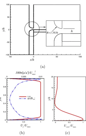
x/h y/h -50 0 50 100 -100 -50 0 50 100 h R=1.583h (a) Uj /Umax 100 u’u’ /U_max2 y/h 0 0.5 1 0 0.005 0.01 0 0.2 0.4 0.6 0.8 1 Uj/Umax u’u’ /Umax2 (b) Uconv /Umax y/h 0 0.5 1 0 5 10 15 20 (c)

Figure 2: (a) Inlet nozzle geometry from the experiment (Rostamy et al. 2011b), (b)

mean streamwise velocity and Reynolds stress at the inlet slot (x/h= 0) and (c)mean convective velocityUconv profile for the outflow boundary condition.

measurements (Rostamy et al. 2011a,b) are also available. However, the mean velocity profile and turbulence measurement at the inlet are not available from Rostamy’s work. They did, however, provide the inlet nozzle geometry (Rostamyet al.2011b) as shown in Figure 2(a). In the current work, a precursor RANS simulation is performed with this two dimensional inlet nozzle to obtain a mean streamwise velocity profile. ANSYS Fluent 14.5, with the standardk−model and default parameters, is used for the RANS simulation. In order to introduce a low level of turbulence at the inlet, a separate channel flow direct numerical simulation is performed at the Reynolds number of Re= Ubulkh

ν = 7500. The mean velocity is removed from the channel flow field and the remaining fluctuations, indicated by the prime symbol, are scaled to achieve a maximum streamwise Reynolds stress hu0u0i/U2

max = 0.01%. The time dependent inflow velocity plane for the DNS is defined using the mean velocity from the precursor RANS calculation, superimposed with the time series of scaled velocity fluctuations from the channel flow. The mean flow and Reynolds stress at the inlet slot of the wall jet are shown in Figure 2(b). For the rest of the inlet plane (1.0₆y/h₆40.0) a uniform streamwise velocity ofU∞= 0.06Uj is defined as a co-flow. This co-flow provides entraining fluid and helps to avoid any large scale circulation in the computational domain. This co-flow is determined systematically using coarse grid simulations with decreasing co-flow magnitude and is lower than previous studies (Zhouet al.1996; Ahlmanet al.2007).

x/h x +, 10 y +, z 0 5 10 15 20 25 30 35 0 5 10 y+ z+ (a) (b) (c) (d)

Figure 3: Quantification of the grid resolution of the current simulations: (a) grid size ∆x+_{, ∆y}+_and∆z+_{distribution along the streamwise direction in wall units,(b)contours} of∆y+_{, the dashed line indicates the location of jet half widthy=y}

1/2,(c)contours of mean grid size∆= (∆x+∆y+∆z)/3.0 with respect to Kolmogorov length scaleη and

(d)actual grid distribution inx−yplane with every 21stpoint in streamwise and every 11thpoint in wall-normal direction is shown.

At the bottom wall of the domain, the no-slip boundary condition is applied i.e.u= v = w= 0. The top wall of the domain has a shear free boundary condition, which is given as ∂u_∂y = ∂w_∂y =v = 0. In the spanwise direction a periodic boundary condition is applied. At the exit plane, the convective outflow boundary condition of Orlanski (1976) is applied, which is given as ∂ui

∂t +Uconv ∂ui

∂x = 0. The mean streamwise velocity profile at the exit plane is used as the convective velocity Uconv. This convective velocity is calculated as a running time average (Lundet al.1998), where the initial transients have to be removed. Figure 2(c)shows a resulting outflow convective velocityUconvprofile at aroundt∗= 1200, which has become statistically steady.

The simulation is performed with 1652×344×302 grid points in the streamwise, wall-normal and spanwise direction, respectively, which results in approximately 172 million cells. This grid is mildly non-orthogonal and non-uniform in thex−yplane, which follows the shear layer development. The grid is uniform in the spanwise direction. There are 78, 188 and 282 wall normal points belowymax,y1/2and 2y1/2, respectively. Figure 3(a) shows the streamwise∆x+_{, wall-normal∆y}+_{and spanwise∆z}+_{grid size variation along} the streamwise direction in the wall units, respectively. The streamwise and spanwise grid sizes are in the range of 5₆∆x+₆10.5 and 8₆∆z+ ₆12, respectively. The wall normal distance of the first grid point is∆y+ <0.7. In the near wall region there are 6 points below y+ = 5 and 12 points below y+ = 11. Figure 3(b) shows the distribution of wall-normal grid size∆y+, which is less than 6 in the active flow region, particularly below the jet half widthy/h < y1/2. The grid size in wall units for the current simulation is comparable to previously reported DNS of wall jets (Ahlman et al.2007; Pouransari

et al.2014) and boundary layer flows (Schlatteret al.2009; Yuan & Piomelli 2015). For the DNS of any turbulent flow, the smallest resolved scale should be of the order ofO(η), whereη = (ν/ε)(1/4)_{is the Kolmogorov length scale and εis the dissipation of} turbulence kinetic energy (Moin & Mahesh 1998). Figure 3(c)shows that the mean grid size with respect to Kolmogorov length scale∆/ηis less than 6, where∆= (∆x+∆y+

u+ tke+ y + 0 5 10 15 20 0 5 10 15 100 101 102 103 u+ (fine) u+ _(coarse) tke+ _(fine) tke+ _(coarse) u /U_max tke y/y 1/ 2 0 0.5 1 0 0.04 0.08 0 1 2 u /Umax (fine) u /Umax (coarse) tke (fine) tke (coarse)

Figure 4: Mean streamwise velocity and turbulent kinetic energy (tke) profiles at x= 30.0hfor coarse and fine grids:(a)outer scaling and(b)inner scaling.

∆z)/3.0. The individual grid size in the streamwise, spanwise and wall-normal directions are ∆x/η < 10, ∆z/η < 10 and ∆y/η < 2, respectively. The current estimates of the grid resolution at the dissipation scales are comparable to the other studies reported in the literature e.g. (Yuan & Piomelli 2015; Moser & Moin 1987). Figure 3(d) shows the actual grid distribution.

An initial simulation was performed with 1250×344×194 grid points, totalling approximately 83 million cells. Figure 4 compares the mean streamwise velocity and turbulent kinetic energy (tke) profiles for the initial and final grids. The comparison is performed with both inner and outer scalings. The velocity profiles do not show any difference. The turbulent kinetic energy profiles have a maximum difference of 3%. All the following results presented in this work are for the final, fine grid.

A fixed time step based on the Courant-Friedrichs-Lewy (CFL) number is used, which is defined as∆t_∆x|u| +_∆y|v| +|_∆zw|= 0.5. This results in a maximum computational time step size of ∆t∗ _{= 0.0015. The simulation is initialized using a uniform flow field with} u= 0.08,v= 0.0 andw= 0.0, which is the streamwise bulk velocity at anyy−z plane of the domain. The flow develops for 1200t∗ to reach a statistically steady state and statistics are collected thereafter for a period of 1300t∗.

3. Results

3.1. Unsteady flow

There are not many examples available in the literature where large scale three dimen-sional structures are presented for wall jets at higher Reynolds numbers. Banyassady & Piomelli (2014) used fluctuating pressure scaled with the maximum local velocity p0/ρU2

max to visualise coherent structures in a wall jet at Rej = 7500. The fluctuating pressure contours in their simulation showed only large roll structures in the outer layer of the fully developed region of the wall jet. In this work, theQ-criterion will be used to identify the large scale structures, which is defined as the second invariant of the velocity gradient tensor∇u.

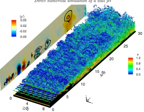
Figure 5 shows an instantaneous picture of large scale vortical structures in the outer layer of the wall jet. Along the outer lip of the wall jet in the shear layer region forx/h <3,

Figure 5: Iso-surfaces of the second invariant of the velocity gradient tensor in the wall jet. The iso-surfaces are coloured with the local streamwise velocityu. Thex−yplane shows the contours of spanwise averaged fluctuating pressure fieldhp0iz and closed streamlines representing the footprint of large scale rotating structures.

Kelvin-Helmholtz instability generates roll structures, which are convected downstream. The roll structures interact with each other and breakdown into smaller more complex structures within a distance ofx/h= 5 from the inlet. These smaller structures undergo a complex motion and farther downstream forx/h >20, structures have some large scale rotation. In order to identify this rotation, time averaged flow variables are subtracted from the instantaneous three dimensional field shown in Figure 5 and fluctuating flow variables are averaged in spanwise direction. Figure 5 shows an x−y plane, with the contours of spanwise averaged fluctuating pressure hp0iz field and streamlines based on spanwise averaged fluctuating velocities hu0iz and hv0iz. The streamlines form closed loops. On moving downstream, these grow in size and move away from the wall with the growth of the outer layer. These closed loop streamlines coincide with the peak values of pressure fluctuationshp0iz and represent the footprint of large scale rotation present in the outer shear layer. Banyassady & Piomelli (2014) used iso-surfaces of fluctuating pressure p0 _{to identify large roll structures in the outer layer region far downstream} beyondx/h >25, similar to the structures identified here.

The near wall inner layer structures are made visible by blanking the flow field above y/h= 0.25. Figure 6 shows the instantaneous inner layer structures. The initial transition region for the inner layer stretches over the range 0 ₆ x/h < 15 and the developed region extends beyond x/h > 20. The transition region shows closely spaced patches of turbulence. These look identical to the turbulence spots appearing in transitional boundary layer flow (Wu & Moin 2009). In the developed region, for x/h > 20, more streamwise aligned tube like structures appear.

Figure 6: Iso-surfaces of the second invariant of the velocity gradient tensor in the inner layer region of the wall jet. The iso-surfaces are coloured with the local streamwise velocity u.

3.2. Global properties

Figure 7(a)shows the decay of maximum mean streamwise velocityUmax of the wall jet as a function of streamwise distance from the jet exit plane on a log-log scale. The current DNS is compared with the power-law given by Tanget al.(2015) and Barenblatt

et al.(2005). The power-law is generally defined as; Umax Uj =Am x h γm . (3.1)

The exponents of the power-law are given by Tang et al. (2015) and Barenblatt et al.

(2005) as γm=−0.482 and−0.6, respectively. The current DNS gives a value ofγm=

−0.4907 beyond x/h= 20, which is within the measured range. Previously it has been assumed that γm = −0.5 (Launder & Rodi 1981; Wygnanski et al. 1992). However, Wygnanskiet al.(1992) suggested that their experimental data fits the power-law better when the exponent is−0.47. This is within 2.5% of the value given by Tanget al.(2015). Narasimhaet al. (1973) reported 4₆Am67 and−0.626γm6−0.49. The maximum streamwise velocity values from the recent LES of Banyassady & Piomelli (2014) are included in Figure 7(a). These are close to the current DNS. Barenblatt et al. (2005) have argued that ifγm 6=−0.5, flow parameters have incomplete similarity or in other words, they depend on the inlet slot height. However, current DNS and several other measurements giveγmclose to−0.5. The value ofγm=−0.6, given by Barenblattet al. (2005) is based on the data of Karlssonet al.(1993), which might be affected by reverse flow (Georgeet al.2000).

x/h

U

/U

LES (Banyassady & Piomelli 2015)

3.55(x/h)-0.4907 3.442(x/h)-0.482 5.150(x/h)-0.6

(a)

y

/h

U

/U

(b)

Figure 7: The decay of maximum mean streamwise velocityUmax as a function of:(a) local streamwise distance from the jet inlet scaled with the slot height and(b)the local half-widthy1/2normalised with the slot height. Current DNS ( ), LES of Banyassady & Piomelli (2014) ( • ). Experimental data: Tanget al.(2015) ( ); Barenblattet al.

(2005) ( ); Georgeet al.(2000) ( ).

noted that there is no theoretical justification for this normalization. However, data from several studies collapse to a power-law given as;

Umax Uj =Bo y_1/2 h n . (3.2)

The exponent of the power-law in Figure 7(b)is given asn=−0.528 and−0.524 based on the measurements by Georgeet al.(2000) and Tanget al.(2015), respectively. These values are within 0.8% of each other. The power-law defined by Georgeet al.(2000) relies on data for x/h _> 40 and for the data of Tanget al. (2015) it is valid for x/h _> 30. However, the current DNS shows that it is in good agreement with these power-laws at axial locations greater than x/h= 25, with the values ofBo= 1.18 andn=−0.542.

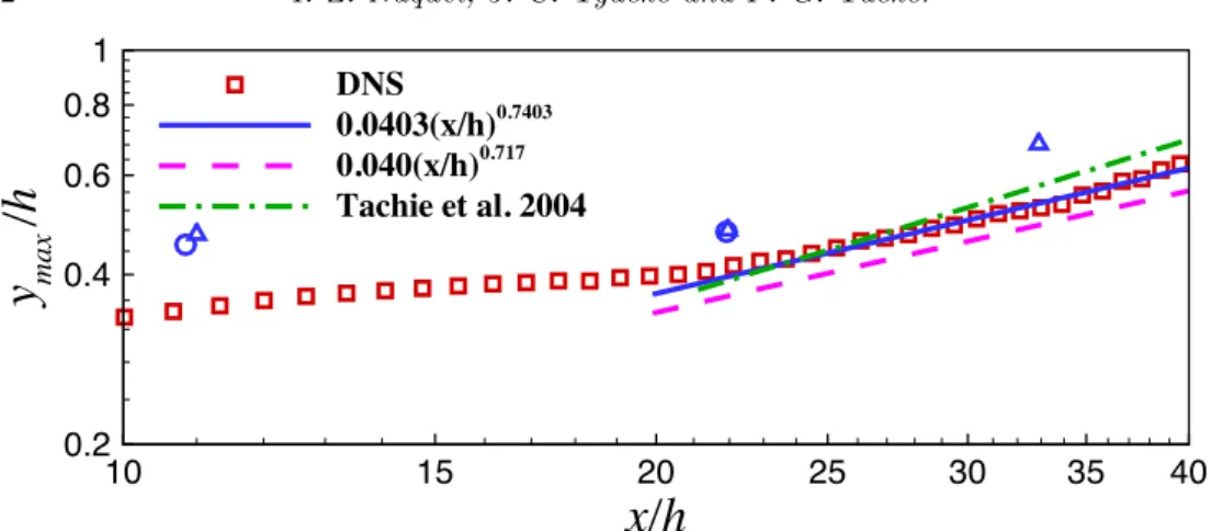
Figure 8 shows the log-log plot of the streamwise variation of the wall-normal location ymax of the maximum streamwise velocity. Tang et al. (2015) defined a power-law relationship forymax/has;

ymax h =Bm x h m . (3.3)

x/h

y

/h

Figure 8: Streamwise development of the wall normal location ymax of Umax. Current DNS ( ); power-law fit to current DNS ( ). Experimental data: Tanget al.(2015) ( ); Tachie et al.(2004), linear fit ( ),Re= 9100 (4),Re= 6100 (◦ ).

The accurate experimental measurement ofymaxis challenging. However, a power-law fit to the current DNS shows that it has the exponent m=−0.7403 as compared to 0.717 measured by Tanget al.(2015). The values ofBmare 0.0403 and 0.040 for the DNS and experiment, respectively. Tachie et al.(2004) have also measuredymax for various inlet Reynolds numbers. The linear fit through their measurements is also included along with two of the representative values atRe= 9100 and 6100, shown by symbols. These are in agreement with the current DNS.

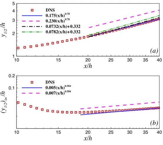
Figure 9 shows the jet spreading rate (or the variation of jet half-width) in the inner and outer layers along the streamwise direction. Barenblatt et al. (2005) have shown that the streamwise development of the half-width in the inner and outer layer regions follow independent scaling laws. The scaling power-laws based on the jet slot height h are defined as;

y1/2 h =Ao x h γo (outer layer), (3.4) and (y1/2)in h =Ai x h γi (inner layer). (3.5)

The outer layer half-widthy1/2is compared with the the power-law given by Tanget al. (2015) based on their experimental data (Figure 9(a)). The power-law fit through the current DNS and Tang et al. (2015) have the same exponent, γo = 0.78. This is 20% lower than the value γo = 0.93 reported by Barenblatt et al.(2005). Other researchers have reported higher values for γo, for example, Narasimha et al.(1973) gave γo= 0.91 and Wygnanskiet al.(1992) 0.88. The coefficientAofor Tanget al.(2015) is 0.230, which is significantly higher than 0.175 for the current DNS. The measured values ofy1/2 are hence greater than the DNS. Linear relationships for half-width have also been defined as y1/2/h= 0.0732(x/h) + 0.332 (Launder & Rodi 1981) andy1/2/h= 0.0782(x/h) + 0.332 (Eriksson et al. 1998), which are closer to the current DNS than the measurements of Tanget al. (2015). The average value of the ratioymax/y1/2 for 256x/h640 is given by current DNS as 0.2, which is higher than a previously reported value of 0.17 (Karlsson

et al.1993).

power-x/h

y

/h

(a)

x/h

(y

)

/h

(b)

Figure 9: Wall jet spreading rate in (a)the outer layer and(b)the inner layer. Current DNS ( ); power-law fit to current DNS ( ). Experimental data: Tanget al.(2015) ( ); Launder & Rodi (1981) ( ); Erikssonet al.(1998) ( ).

law given by Tanget al. (2015). The power-law fit through the DNS data has the same exponent γi = 0.504 as the measurements (Tang et al. 2015). Barenblatt et al. (2005) gave the power-law exponentγi= 0.68, which is 20% higher than the current value. The coefficientAi = 0.005 for the DNS is lower than the measured value of 0.007 (Tanget al. 2015). The measured data hence produces higher values of (y1/2)in than the DNS.

Figure 10(a) shows the streamwise evolution of wall shear stressτw = µ ∂u/∂y|_y=0, where µ is the dynamic viscosity of the fluid. The scaling used here is defined by Narasimha et al.(1973), which uses the initial kinetic momentum fluxMo=R

h 0 Uj

2_dy, kinematic viscosity and density to scale wall shear stress. This approach eliminates the effect of inflow Reynolds numberRej on the scaling. The power-law form for this scaling is given as; τwν2 ρMo2 =Aτ _xM o ν2 γτ . (3.6)

The exponent for the power-law fit through the current DNS isγτ =−0.967. The value ofγτbased on measurements is given as−1.053 and−1.07 by Rostamyet al.(2011b) and Wygnanski et al. (1992), respectively. These values are within 10% of each other. The coefficientAτ is determined to be 0.03, 0.161 and 0.146 for the current DNS, Rostamy

xM

/

w

2

/M

o

2

1E+09 1.5E+09 2E+09

10-12 10-11 10-10

DNS

LES (Banyassady & Piomelli 2014) 0.03(xM_o / 2)-0.967 0.161(xM_o / 2)-1.053 0.146(xM_o / 2)-1.070

_(a)

Re

=U

y

/

C

LES (Banyassady & Piomelli 2015) Eriksson et al. 1998

Tachie et al. 2004 Rostamy et al. 2011b

George et al. 2000

(b)

Figure 10: (a)Streamwise development of the wall shear stress scaled with momentum-viscosity scaling. Current DNS ( ); power-law fit to current DNS ( ). LES of Banyassady & Piomelli (2014) (•). Experimental data: Rostamyet al.(2011b) ( ); Wygnanskiet al.(1992) ( ).(b) Variation of skin friction coefficientCf with local Reynolds numberRem=Umaxymax/ν. Current DNS ( ). LES of Banyassady & Piomelli (2015) ( • ). Experimental data: Eriksson et al. (1998) (4); Tachie et al. (2004) (5); Rostamyet al.(2011b) (◦); Georgeet al.(2000) ( ).

et al.(2011b) and Wygnanskiet al.(1992), respectively. The wall shear stress predicted with LES (Banyassady & Piomelli 2014) is close to the current DNS.

Figure 10(b)shows the log-log plot of skin friction coefficientCf against local Reynolds numberRem= Umax_νymax.Cf is defined as;

Cf = 2 τw ρU2 max = 2 _u τ Umax 2 . (3.7)

The local Reynolds number Rem in the developed region ranges from 2500−3100 for the current DNS. The predicted values ofCf are in agreement with several experimental studies (Eriksson et al. 1998; Tachieet al. 2004; Rostamy et al. 2011b). George et al.

(2000) gave a theoretical relation for friction velocity based on a power law. This can be used to determine the skin friction coefficient variation againstRem. This relationship is also included in Figure 10(b). The current DNS approaches asymptotically to it beyond

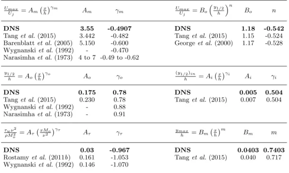
Umax Uj =Am x h γm Am γm Umax_U j =Bo y_1/2 h n Bo n DNS 3.55 -0.4907 DNS 1.18 -0.542

Tanget al.(2015) 3.442 -0.482 Tanget al.(2015) 1.15 -0.524 Barenblattet al.(2005) 5.150 -0.600 Georgeet al.(2000) 1.17 -0.528 Wygnanskiet al.(1992) - -0.470 Narasimhaet al.(1973) 4 to 7 -0.49 to -0.62 y_1/2 h =Ao x h γo Ao γo (y_1/2)in h =Ai x h γi Ai γi DNS 0.175 0.78 DNS 0.005 0.504

Tanget al.(2015) 0.230 0.78 Tanget al.(2015) 0.007 0.504 Wygnanskiet al.(1992) - 0.88 Narasimhaet al.(1973) - 0.91 τwν2 ρM2 o =Aτ xMo ν2 γτ Aτ γτ ymax_h =Bm x_h m Bm m DNS 0.03 -0.967 DNS 0.0403 0.7403

Rostamyet al.(2011b) 0.161 -1.053 Tanget al.(2015) 0.040 0.717 Wygnanskiet al.(1992) 0.146 -1.070

Table 1: Various power-laws for wall jets.

Rem= 2800. Banyassady & Piomelli (2015) have reportedCf for a significantly longer range of Rem based on their LES, however, their reported values are higher than the current predictions.

Various power-laws for the wall jet discussed in this section are summarised in Table 1.

3.3. Mean flow and turbulence statistics

3.3.1. Mean velocity

Figure 11(a) shows mean streamwise velocity profiles at x/h = 25, 30 and 35. The profiles are scaled with the outer parameters y1/2 and Umax. For the given range in the streamwise direction, the profiles show self-similar behaviour. Erikssonet al.(1998) showed that the mean streamwise velocity profiles show self-similar behaviour in outer scales beyond x/h = 20. The mean flow predicted by previous LES (Banyassady & Piomelli 2014) is in agreement with the DNS. The current results also compare well with the measurements of Rostamyet al.(2011a) and Erikssonet al.(1998). This is with the exception of close to the edge of outer layer beyond y/y1/2 > 1.8. This is due to the difference in outer flow conditions. The experiments have reverse flow for entrainment.

In the presence of a weak co-flow with the velocity U∞, the outer scaling for the mean streamwise velocity is defined as hui−U∞

Umax−U∞ (Irwin 1973; Zhouet al.1996) andy1/2

is located where hui = 1₂(Umax−U∞). Figure 11(b) shows that the mean streamwise velocity profiles at x/h = 25, 30 and 35 collapse with this scaling in the outer layer region. The velocity profiles are compared with the experimental data of Irwin (1973) at

u /Umax y/y 1/ 2 0 0.2 0.4 0.6 0.8 1 0 1 2 x=25h x=30h x=35h

(a) ( u -U )/(Umax-U )

y/y 1/ 2 0 0.2 0.4 0.6 0.8 1 0 1 2 x=25h x=30h x=35h (b)

Figure 11: Mean streamwise velocity profiles scaled with outer length scales(a)hui/Umax and(b)(hui −U∞)/(Umax−U∞). LES of Banyassady & Piomelli (2014) (•),x= 30h. Experimental data: Rostamy et al. (2011a) ( ◦ ), x= 30h; Erikssonet al. (1998) (4), x= 40h; Irwin (1973) (5),x= 82.2h. v /(Umax-U ) y/y 1/ 2 -0.05 0 0.05 1 2 x=25h x=30h x=35h

Figure 12: Mean wall normal velocity profiles scaled with outer parameters. Experimental data: Erikssonet al.(1998) (4),x= 70h.

Figure 12 shows the outer scaled mean wall normal velocityhvi. The velocity profiles do not collapse beyond y/y1/2 = 1.2. The calculated wall normal velocity is in good agreement with the measurements of Eriksson et al. (1998) up to y/y1/2 = 1.6. The difference in measurements and computed values in the outer region is again due to different entrainment conditions.

Figure 13 shows the inner scaled mean streamwise velocity hui+ _{profiles in a} semi-logarithmic form. The computed profiles at three streamwise locationsx/h= 25, 30 and 45 collapse up toy+_{= 300. The current DNS is in agreement with the experimental data} (Rostamyet al.2011a; Erikssonet al.1998). The LES of Banyassady & Piomelli (2014) gives slightly lower values forhui+ _{in the range of 10}

6y+

6370, than the current DNS. There is agreement with the linear profilehui+_=y+_belowy+_{= 4, which is similar to the} flat plate turbulent boundary layer (Wu & Moin 2009). The near wall velocity profiles for wall bounded flows are also expressed as a log-law of the formhui+_{=A ln(y}+_{) +B. The} current DNS is compared with a log-law havingA= 2.44 andB= 5.0. These constants

y

u

2.44 ln(y

)+5.0

Figure 13: Inner scaled mean streamwise velocity profiles hui+_{. Log-law hui}+ ₌ 2.44ln(y+_{) + 5.0 ( ). Linear profile hui}+ _{= y}+ _{( · · · · ). LES of Banyassady} & Piomelli (2014) ( • ), x = 30h. Experimental data: Rostamy et al. (2011a) ( ◦ ), x= 30h; Erikssonet al.(1998) (4),x= 40h. u /U_max Ao [y /y1/ 2 ] 0 0.2 0.4 0.6 0.8 1 0.1 0.2 0.3 0.4 x=25h x=30h x=35h (a) u /U_max Ai [y /( y1/2 )in ] 0 0.2 0.4 0.6 0.8 1 10-3 10-2 10-1 100 x=25h x=30h x=35h (b)

Figure 14: Mean streamwise velocity profiles scaled with incomplete similarity parameters of Barenblattet al.(2005):(a)outer scaled profiles and(b)inner scaled profiles.

are the generally accepted values for flat plate turbulent boundary layers (Spalart 1988). Several previous experimental measurements of wall jets (Erikssonet al.1998; Rostamy

et al. 2011a; Tachie et al. 2004) have shown agreement with these log-law parameters. Erikssonet al.(1998) showed that their measurements are in agreement with the log-law in the range of 30 ₆ y+

680, whereas the current DNS range is 20 ₆ y+

6 90. The log-law parameters for the LES (Banyassady & Piomelli 2014) areA= 2.22 andB= 5.0. Figure 14 represents mean streamwise velocity profiles with incomplete similarity parameters described by Barenblatt et al. (2005). The outer scaling parameters for incomplete similarity are traditionally defined except for the factorAo used for scaling they−axis (Figure 14(a)). The parameter Ao is given in equation 3.4, which describes the dependence of the outer layer length scaley1/2 on the streamwise distancex/h. The semi-logarithmic plot clearly shows that outer scale mean streamwise velocity profiles above ymax show perfect collapse, whereas profiles below ymax diverge. Figure 14(b) shows the inner scaled profiles of mean streamwise velocity. The y−axis is scaled with Ai and (y1/2)in given in equation 3.5. The inner scaling is able to collapse the velocity profile in the inner layer region belowymax. Barenblattet al.(2005) gave a relationship for mean streamwise velocity based on incomplete similarity as;

hui=      M ρh 12 _x h γm ψu _h1−γoyxγo,Re , ify > ymax; M ρh 12 _x h γm ψu _h1−_γiy_xγi,Re , ify < ymax. (3.8)

ψu is a function of length scales and Reynolds number. Earlier it was shown that the current DNS and several recent measurements give γm close to −0.5, which results in a weak dependence on inlet slot height and hence at high Reynolds number complete similarity is possible. It is important to point out that even if the hypothesis of incomplete similarity is not applicable for the wall jet, the inner layer parameters of equation (3.5) suggested by Barenblattet al.(2005) show the same quality of scaling as the inner scaling suggested by George et al.(2000), based on the asymptotic invariance principle (AIP). It can be shown that the parameters given in equation (3.5) are consistent with the similarity theory of Georgeet al.(2000). The detailed derivation is given in Georgeet al.

(2000), here the essential relationships are referenced to check the scaling parameters. It has been shown (George et al.2000) that at infinite Reynolds number the momentum equation in the inner layer region is given as;

∂ ∂y h−u0v0i+ν∂hui ∂y = 0 (3.9)

wherehui= 0 aty= 0. Equation (3.9) can be integrated to obtain

h−u0v0i+ν∂hui ∂y =

τw

ρ =uτ (3.10)

The form of similarity solution is given as

hui=Usi(x)fi∞(ysi) (3.11)

h−u0v0i=Rsi(x)ri∞(ysi) (3.12) whereUsi,fi∞,Rsiandri∞are spatial functions.ysi=y/lsiand length scalelsi=lsi(x) is required for proper scaling. Substituting these solutions in equation (3.10) gives

_u2 τ U2 si = _R si U2 si ri∞+ _ν lsiUsi f_i0_∞. (3.13)

For the similarity solution all the bracketed terms should have same x−dependence i.e. _u2 τ U2 si ∼ _R si U2 si ∼ _ν lsiUsi . (3.14)

It has been shown by Georgeet al.(2000) that if the length scale is defined aslsi=_Uν si, uτ must be the inner velocity scale. Now if we use inner length scale defined in (3.5) i.e.lsi= (y1/2)in, then any appropriate velocity can be used for the scaling. In this case Umax is the obvious choice and Figure 14(b) clearly shows that these parameters are appropriate scales in the inner layer region. The only other requirement from the George

et al. (2000) similarity theory is that the Reynolds shear stress should also scale with Umax and (y1/2)inin the inner layer region, which is shown in the next section.

3.3.2. Reynolds stresses

Figure 15 shows outer scaled Reynolds normal and shear stress profiles at streamwise locationsx/h= 25, 30 and 35. The normal and shear stresses are normalized by (Umax− U∞)2. The streamwisehu0u0i, wall normalhv0v0iand shear stresseshu0v0ifrom the current

u’u’ /(Umax-U ) 2 y/y 1/ 2 0 0.02 0.04 0.06 0 1 2 x=30h x=35h x=40h (a) v’v’ /(Umax-U ) 2 y/y 1/ 2 0 0.02 0.04 0 1 2 x=25h x=30h x=35h (b) w’w’ /(U_max-U )2 y/y 1/ 2 0 0.02 0.04 0 1 2 x=25h x=30h x=35h (c)

u’v’ /(U_max-U )2

y/y 1/ 2 -0.010 0 0.01 0.02 1 2 x=25h x=30h x=35h (d)

Figure 15: Outer scaled Reynolds normal and shear stress profiles:(a)streamwisehu0u0i;

(b)wall-normalhv0v0i;(c)spanwisehw0w0iand(d)shear stresshu0v0i. LES of Banyassady & Piomelli (2014) ( • ), x = 30h. Experimental data: Rostamy et al. (2011a) ( ◦ ), x= 30h; Erikssonet al.(1998) (4),x= 40h; Irwin (1973) (5),x= 82.2h.

DNS are compared with the measurements of Eriksson et al. (1998) at Rej = 9600, Rostamy et al. (2011a) at Rej = 7500 and the LES of Banyassady & Piomelli (2014) also atRej = 7500. The DNS results are close to the reported LES and slightly higher than the measurements of Eriksson et al. (1998). These measurements are at a higher Reynolds number than the current DNS. Note, Wygnanski et al. (1992) showed that with increasing Reynolds number, outer scaled values of hu0u0i decrease slightly. The experimental data of Rostamy et al. (2011a) gives higher values for all the stresses at the same Reynolds number as the current DNS. It is important to note here that the current DNS relies solely on transition and resolution of the production mechanism for turbulence generation. On the other hand, the LES of Banyassady & Piomelli (2014) used forcing at streamwise locations x/h= 2, 4, 6 and 8 in the wall normal momentum equation. This gave Reynolds shear stress profiles equal to the measurements of Rostamy

et al.(2011a) at these locations. Beyond the forcing planes, the LES allowed the flow to evolve naturally, however, even with this forcing, predicted stresses are still lower than the measurements. A possible reason for the higher values of Reynolds normal and shear stresses of Rostamyet al.(2011a) might be the uncertainties in the measurement of their scaling parameters. Figure 15(c) shows the outer scaled Reynolds stress profiles in the spanwise directionhw0w0i. Few experimental studies have measuredhw0w0i, however, the current DNS shows agreement with the measurements of Irwin (1973) atRej= 28000.

It has been shown by several experimental studies (Irwin 1973; Abrahamsson et al.

and shear stress profiles exhibit self-similar behaviour with outer scaling in the developed region of the wall jet. The Reynolds stresses have shown self similarity as early asx/h= 30 (Rostamy et al.2011a). The outer scaled Reynolds normal and shear stress profiles from the current DNS in Figure 15 do not show the same level of collapse as the mean streamwise velocity profiles in Figures 11 or 14. However, the maximum differences in the peak values for these DNS profiles atx/h= 30 and 35 are less than the experimental uncertainty given by Rostamyet al.(2011a).

Figure 16 shows the inner scaled Reynolds normal and shear stress profiles. The friction velocity uτ and inner length scale ν/uτ are the velocity and length scales. Again, the streamwisehu0u0i+_{, wall normalhv}0_v0_i+_{and shear stresshu}0_v0_i+_{profiles from the current} DNS are compared with the experimental data of Eriksson et al. (1998) and Rostamy

et al. (2011a) and the LES of Banyassady & Piomelli (2014). The measurements of Eriksson et al. (1998) and LES are close to the current DNS for hv0v0i+ _{and hu}0_v0_i+ and lower for hu0u0i+ _{in the inner layer region. The inner layer region extends up to} y/y1/2= 0.2, ory+= 160. The measurements of Rostamyet al.(2011a) are significantly higher than the current DNS for hu0_u0_i+ _{and hv}0_v0_i+_{, whereas hu}0_v0_i+ _{is in agreement.} Thehv0v0i+_andhu0_v0_i+_{profiles atx/h= 25, 30 and 35 collapse in the inner layer region.} Whereas hu0u0i+ _{and hw}0_w0_i+ _{have a small variation, this is less than the uncertainty} levels in the measurements (Rostamy et al. 2011a). Figure 16(d) also compares the velocity gradient profile y+dhui+

dy+ at x = 30h, with the Reynolds shear stress. The velocity gradient becomes zero at y = ymax or y+ = 161, where the Reynolds shear stress has a finite positive value. Moreover, for a narrow region belowy=ymaxboth the velocity gradient and Reynolds shear stress are positive. This invalidates the Boussinesq hypothesis hu0v0i=_−ν

T ∂hui

∂y for the wall jet, where the positive scalar coefficient νT is the turbulent viscosity. It also shows that the positive shear stress from the outer layer is transported against the velocity gradient belowy=ymaxdue to the turbulence transport. Georgeet al.(2000) showed, using the asymptotic invariance principle (AIP), that for correct outer scaling, the shear stresshu0v0ishould be normalised with the shear velocity u2

τ. Figure 17(a)shows the shear stress profiles with this scaling. The profiles atx/h= 30 and 35 show an improvement in their collapse with respect to this new scaling (George

et al.2000) relative to the scaling based on a single velocity and length scale (Irwin 1973). This can be seen in Figure 15(d). The current scaled profiles are in agreement with the experimental data of Erikssonet al.(1998) up toy/y1/2= 0.8. Beyond this, experimental values forhu0v0i+ _{are higher. This might be due to the higher Reynolds number for the} experiment and difference in wall friction velocity.

Figure 17(b)shows the shear stress profiles scaled with incomplete similarity parame-ters (Barenblattet al.2005). It has been discussed earlier that the incomplete similarity parameters for the inner layer region would be consistent with the asymptotic invariance principle (George et al.2000), if they scale the Reynolds shear stress. The figure shows a good collapse of shear stress profiles with this scaling in the inner layer region.

The instantaneous values of velocity and pressure are saved at selected wall normal locations atx/h= 30, for each time step fromt∗= 1200 to 2500, giving 860000 samples. Note, St = f h/Uj is the Strouhal number or non-dimensional frequency and f is the frequency. As shown in Figure 18, the streamwiseEu0 and wall-normal E_v0 spectra are

given aty+ _{= 5 (y/y}

1/2 = 0.006), y+ = 17 (y/y1/2= 0.02),y/y1/2= 0.2 and y/y1/2= 0.8. These locations represent the end of the linear region in the viscous sub layer, the first peak in hu0u0i, Umax and the outer layer peaks in hu0u0i and hv0v0i, respectively. The Reynolds stresshu0u0ihas a lower value at y+ _{= 5, and contains less energy at the} smaller scales relative to the other locations (Figure 18(a)). At the other three locations

y

u’

u’

(a)

y

v’

v’

(b)

y

w’

w’

(c)

y

u’

v’

(d)

Figure 16: Inner scaled Reynolds normal and shear stress profiles(a)streamwisehu0u0i+_,

(b) wall-normalhv0v0i+_{, (c) spanwisehw}0_w0_i+ _{and(d)shear stresshu}0_v0_i+ _{and velocity} gradient y+d_dyhui++ at x = 30h. LES of Banyassady & Piomelli (2014) ( • ), x = 30h. Experimental data: Rostamy et al. (2011a) ( ◦ ), x= 30h; Erikssonet al. (1998) (4), x= 40h.

u’v’+ y/y 1/ 2 -1 0 1 2 3 4 0 1 2 x=25h x=30h x=35h (a)

u’v’ /(U_max-U )2

Ai [y /( y1/2 )in ] 0 0.01 0.02 10-3 10-2 10-1 100 x=25h x=30h x=35h (b)

Figure 17: (a) Correct scaling of shear stress profile according to George et al. (2000). Experimental data: Erikssonet al.(1998) (4),x= 40hand (b) inner scaled shear stress profiles with respect to incomplete similarity parameters (Barenblattet al. 2005).

St=fh/U_j Eu’ 10-2 10-1 100 101 10-8 10-7 10-6 10-5 10-4 10-3 10-2 10-1 100 St-5/3 St-7 (a) St=fh/U_j Ev’ 10-2 10-1 100 101 10-8 10-7 10-6 10-5 10-4 10-3 10-2 10-1 100 St-7 St-5/3 (b) St=fh/U_j Ew’ 10-2 ₁₀-1 ₁₀0 ₁₀1 10-8 10-7 10-6 10-5 10-4 10-3 10-2 10-1 100 St-7 St-5/3 (c) St=fh/U_j Ep’ 10-2 ₁₀-1 ₁₀0 ₁₀1 10-8 10-7 10-6 10-5 10-4 10-3 10-2 10-1 St-7 St-5/3 (d)

Figure 18: Frequency spectra of velocity and pressure fluctuations at x/h = 30 (a)

streamwiseEu0 at:y+= 5 ( );y+= 17 ( );y/y_1/2= 0.2 ( );y/y_1/2= 0.8

( ), (b) wall-normal Ev0 at: y+ = 5 ( ); y+ = 17 ( ); y/y_1/2 = 0.2 (

);y1/2= 0.8 ( ),(c) spanwise Ew0 at: y+ = 5 ( );y+ = 40 ( );

y/y1/2= 0.2 ( );y/y1/2= 0.8 ( ) and (d)pressureEp0 at:y+= 5 ( );

y+_{= 17 ( );y/y}

huuivalues are close to each other and so too are the spectra. The wall-normal Reynolds stress hv0v0i increases continuously from the wall to a peak value around y/y1/2 = 0.8. Correspondingly spectra at increasing wall distance indicate a higher energy level. The spanwise velocity fluctuation spectraEw0 (Figure 18(c)) are given at the same locations

as Eu0 and E_v0, except for y+ = 40 (y/y_1/2 = 0.05), which is the first near wall peak

in hw0w0i. The streamwise velocity fluctuation spectra show a −5/3 slope in the range of 0.06 < St < 2.0 in the outer layer region. The wall-normal and spanwise velocity fluctuations spectra have a−5/3 slope in a smaller range of frequencies 0.4 < St <2.0 in the outer layer region. The higher frequency region is the viscous sub range, where dissipation occurs and spectra can be compared to a line with a slope of -7. The spectra in the inner layer region are closer to such a line as compared to the outer layer region.

In the low frequency region below St < 0.06 spectra, particularly for Eu0 and E_v0,

peaks indicating large scale fluctuations in the flow can be observed. Figure 18(d)shows the pressure spectraEp0 at identical locations to the spectra forE_u0 andE_v0. The main

features in the pressure spectra are multiple peaks in the low frequency range forSt < 0.06, as observed forEu0 and E_v0. The peaks appear to be the signature of large scale

structures passing in the outer layer region identified in Figure 5.

3.4. Reynolds stresses and turbulence energy balance

An objective here is to present reliable turbulence kinetic energy tke and Reynolds stresses budgets. The budgets are compared with a previously reported LES of Dejoan & Leschziner (2005). This LES is performed on a much coarser grid than the current DNS. The total number of LES grid points is more than an order of magnitude smaller than the DNS. The LES grid spacing, in stramwise and spanwise directions, is twice that of the current DNS. The dynamical equation for the Reynolds stress tensor in its non-dimensionalized form is given as;

Chu0 iu 0 ji=Phu 0 iu 0 ji+εhu 0 iu 0 ji+Thu 0 iu 0 ji+Ψhu 0 iu 0 ji+Dhu 0 iu 0 ji (3.15)

where the following terms appear in this equation, with summation on repeated indices,

Chu0 iu0ji=huki ∂hu0_iu0_ji ∂xk Convection Phu0 iu0ji=−hu 0 ju 0 ki ∂huii ∂xk − hu0_iu0_ki∂huji ∂xk Production εhu0 iu 0 ji=− 2 Re _∂u0 i ∂xk ∂u0 j ∂xk Dissipation Thu0 iu 0 ji=− ∂hu0_iu0_ju0_ki ∂xk Turbulent diffusion Ψhu0 iu 0 ji=− u0j ∂p0 ∂xi − u0i ∂p0 ∂xj

Velocity-Pressure gradient correlation

Dhu0 iu0ji= 1 Re ∂2_hu0 iu0ji ∂xk∂xk Viscous diffusion

Note,tke= 1₂(hu0u0i+hv0v0i+hw0w0i), and its budget can be calculated by summing the budgets of individual Reynolds normal stresses given by equation 3.15.

3.4.1. Inner-scaled budgets

Figure 19 shows the budgets fortke, Reynolds normal and shear stresses atx/h= 30 in the inner layer region. The profiles are scaled with the inner variables, whereas the

y

L

os

s G

ai

n

tke

(a)

y

L

os

s G

ai

n

u’u’

(b)

y

L

os

s G

ai

n

v’v’

(c)

y

L

os

s G

ai

n

w’w’

(d)

y

L

os

s G

ai

n

u’v’

(e)

Figure 19: Turbulence kinetic energy (tke), Reynolds normal and shear stress budgets in the near wall region. The terms are normalised with u4

τ/ν: (a) tke= (hu0u0i+hv0v0i+

hw0w0i)/2;(b)hu0u0i; (c)hv0v0i;(d)hw0w0iand(e) hu0v0i. LES of wall jet by Dejoan & Leschziner (2005): Production (_N); dissipation ( ); velocity-pressure gradient correlation ( • ); turbulent diffusion (_H). DNS of turbulent boundary layer by Spalart (1988): Production (4); dissipation ( ); velocity-pressure gradient correlation ( ◦ ); turbulent diffusion (5).

budget terms are normalised withu4

τ/ν. The balance or the sum of all the budget terms for each Reynolds stress is O(10−2) of the maximum value. As mentioned earlier, the current budgets are compared with the wall jet LES of Dejoan & Leschziner (2005). This LES might be the only published budget for comparison for wall jets in the inner layer region. The LES based budget is given atx/h= 20 and only the dominant terms from that budget are included here. The dominant terms of the turbulence kinetic energy and Reynolds stress budgets from the flat plate turbulent boundary layer DNS of Spalart

(1988) are also included in Figure 19. This helps to understand how closely the inner layer of the plane wall jet follows a turbulent boundary layer flow.

It is clearly shown that (Figure 19(a),(b),(d)and(e)) the dominant terms of produc-tion, dissipation and velocity-pressure gradient correlation for turbulent kinetic energy, Reynolds streamwise, spanwise and shear stress budgets for the wall jet and boundary layer are in agreement. The wall normal Reynolds stress budget shows (Figure 19(c)) that the dominant terms of dissipation and velocity-pressure gradient correlation have different peak values from the boundary layer, however the trend is the same for both flows. The turbulent transport term for the wall normal and shear stress budgets indicate a major deviation of the wall jet from the turbulent boundary layer. This has a significant effect on the Reynolds wall normal and shear stress distribution of wall jet.

In Figure 19(a)a comparison of thetkebudget with previously reported LES (Dejoan & Leschziner 2005) shows that the level of production is lower than the current DNS and the trend for the dissipation does not match below y+ _{= 20. The Reynolds wall} normal and shear stress budgets (Figure 19(c)and(e)) from LES show even more drastic deviation from the current DNS. In the case of Reynolds shear stress the LES gives a significantly lower level of production and velocity-pressure gradient correlation. The wall normal stress from the LES does not follow standard wall behaviour, rather than velocity-pressure gradient correlation term it gives turbulent transport as the dominant term, which is balanced by the dissipation. Moreover, the trend for turbulent transport and level of dissipation for wall normal stress from LES do not match with the current DNS. A possible explanation is that the LES predicted these budgets atx/h= 20, where the wall jet boundary layer may not be fully developed and the outer shear layer is interacting with the wall. However, the current DNS shows that the velocity-pressure gradient term is dominant for thehv0_v0_{ibudget in the inner layer region as far upstream} as x/h = 15. Also, the dissipation term in the LES is not calculated explicitly, but evaluated as a balance from the rest of the terms. This might be responsible for the near wall difference belowy+ _{= 20 in hu}0_u0_{i, where sub-grid modelling may have some} deficiencies. The overall difference between the current DNS and LES is due to the lower grid resolution of the latter, as mentioned earlier.

For the DNS, as can be seen from Figure 19(a)in the inner layer region, the turbulent kinetic energy budget shows that the dissipation is balanced by viscous diffusion in the viscous sub-layer for y+ _{<5. The production term has high values outside the viscous} sub-layer in the range of 5₆y+

650, with a peak around y+_{= 12. This high value of} production is balanced mainly by dissipation and up to a certain extent, by turbulence diffusion. Eriksson (2003) estimated the near wall dissipation value as 0.27, which is 12% lower than the current value of 0.31.

Figure 19(b) shows the streamwise Reynolds stress hu0u0i budget. This is similar to the turbulence kinetic energy budget, except for the velocity-pressure gradient correlation term. This changes the sign and balances production along with dissipation and turbulent diffusion. The velocity-pressure gradient correlation transfers streamwise energy to other directions. The high level of production in the region of 5 ₆ y+

6 50 is responsible for the inner layer peak of the streamwise Reynolds stress (Figure 16(a)). For the wall normal stress hv0v0i budget in the inner layer region (Figure 19(c)), the dissipation is mainly balanced with the velocity-pressure gradient correlation and turbulent diffusion terms. The production is small and wall normal turbulence in the inner layer region is maintained by turbulent diffusion and velocity-pressure gradient correlation. These transfer turbulence energy from the streamwise to the wall normal direction. Figure 19(d)

shows the budget for the spanwise Reynolds stress hw0w0i. The dissipation is balanced by viscous diffusion in the viscous sub-layer region y+ < 5. Outside the viscous

sub-layer, it is balanced with the velocity-pressure gradient term. The Reynolds shear stress

hu0v0i budget (Figure 19(e)) has high negative production, which is balanced by the velocity-pressure gradient term and turbulent diffusion.

3.4.2. Outer-scaled budgets

Figure 20 shows the turbulence kinetic energy, Reynolds normal and shear stress budgets at x/h= 30 in the outer layer region. The budget terms are normalised with (Umax−U∞)3 and wall normal distance with y1/2. The balance for the outer scaled budgets is less than 4% of the peak values of production and dissipation. The outer scale LES budgets of Dejoan & Leschziner (2005) are compared with the current DNS. The predicted turbulence kinetic energy budget is also compared with the measurements of Irwin (1973) and Zhouet al.(1996).

Figure 20(a) shows the outer scaled turbulent kinetic energy budget, where all the terms have been evaluated explicitly for the current DNS. The viscous diffusion and velocity-pressure gradient terms are negligible in the outer layer region. The production and convection terms are mainly balanced by turbulent diffusion and dissipation. The production term has a minima around ymax, however it always remains positive. The production, dissipation and turbulent transport terms are compared with the mea-surements. In the experiments only turbulent transport can be measured directly and the DNS values lie between the two sets of measurements (Irwin 1973; Zhou et al.

1996) and is closer to Irwin’s data. In experiments the production is estimated from a mean curve drawn through the measured mean velocity values (Irwin 1973). Both experiments cited here give identical values of production and are close to the current DNS. The dissipation is estimated either from local spectra using the −5

3 law (Irwin 1973) or using the assumption of local isotropy along with Taylor’s hypothesis (Zhou

et al.1996). The dissipation estimates from Irwin (1973) are close to the current DNS, where as Zhou et al. (1996) have estimated a higher level of dissipation. The current DNS shows that the assumption of isotropy in dissipation is not valid in the inner layer region below y/y1/2 = 0.2 = ymax. The DNS shows that in the outer layer region for 0.2 ₆y/y1/2 61 the wall normal dissipation

D ∂v0 ∂xk ∂v0 ∂xk E is 15%−20% smaller and the spanwise dissipation D_∂x∂w0

k ∂w0 ∂xk

E

is 10%−15% smaller than the streamwise dissipationD_∂x∂u0

k ∂u0 ∂xk

E

, respectively. The dominant terms of production and velocity-pressure gradient correlation from LES (Dejoan & Leschziner 2005) are slightly lower than the current DNS, where as the dissipation is in good agreement for various budgets.

Figure 20(b)shows the outer scaled streamwise Reynolds stresshu0u0ibudget. The pro-duction has high positive values in the range of 0.2< y/y1/2<1.5, which is responsible for high values of Reynolds stresshu0_u0_{iin the outer layer region. A portion of this energy} is dissipated and the remainder transfers to turbulent and velocity-pressure gradient diffusion. The turbulent production has a minimum value at ymax, where maximum mean velocity occurs and ∂hui/∂y = 0. At this location, turbulence is maintained by the turbulent diffusion term. This transports the turbulence energy from the outer high energy region. The velocity-pressure gradient diffusion term transfers energy from the streamwise direction to the wall normal and spanwise turbulence components. The wall normal Reynolds stresshv0v0ihas little production in the outer layer region (Figure 20(c)). The turbulence is mainly driven by the velocity-pressure gradient correlation term, which is balanced by the dissipation and turbulent diffusion terms. The spanwise Reynolds stresshw0w0ibudget shows that the velocity-pressure gradient and convection terms are

+ + + + + + + + + + + + + * * * * * * * * * * * * * * * * * * * *

y/y

L

os

s G

ai

n

(a)

tke

y/y

L

os

s G

ai

n

(b)

u’u’

y/y

L

os

s G

ai

n

v’v’

(c)

y/y

L

os

s G

ai

n

w’w’

(d)

y/y

L

os

s G

ai

n

(e)

u’v’

Figure 20: Turbulence kinetic energy (tke), Reynolds normal and shear stress budgets in the outer layer region. The terms are normalised with (Umax−U∞)3/y1/2. Legends for DNS are same as in Figure 19.(a)tke= (hu0u0i+hv0v0i+hw0w0i)/2,(b)hu0u0i,(c)hv0v0i,

(d)hw0w0iand(e)hu0v0i. LES of wall jet by Dejoan & Leschziner (2005): Production (_N); dissipation ( ); velocity-pressure gradient correlation ( • ). Experimental data, Irwin (1973): Production (4); dissipation ( ); turbulent diffusion (+) and Zhouet al.(1996): Production (5); dissipation (); turbulent diffusion (∗).

balanced with the dissipation and turbulent diffusion terms in the outer layer region (Figure 20(d)). The turbulent diffusion term transfers energy from the outer layer region to the inner layer maintaining turbulence aroundymax.

The shear stress budget hu0v0i has the production and velocity-pressure gradient as the dominant terms, which balance each other (Figure 20(e)). In the outer layer region, production is positive and is responsible for high values of shear stresshu0v0i. Aty=ymax the velocity gradient and production become zero and below this point production is negative, however shear stress remains positive for some distance in this region. The