Gnani, F., Zare-Behtash, H., White, C. and Kontis, K. (2018) Numerical
investigation on three-dimensional shock train structures in rectangular
isolators.
European Journal of Mechanics - B/Fluids
, 72, pp. 586-593.
(doi:
10.1016/j.euromechflu.2018.07.018
)
This is the author’s final accepted version.
There may be differences between this version and the published version.
You are advised to consult the publisher’s version if you wish to cite from
it.
http://eprints.gla.ac.uk/167975/
Deposited on: 03 September 2018
Enlighten – Research publications by members of the University of Glasgow http://eprints.gla.ac.uk
Numerical Investigation on Three-dimensional Shock Train
1
Structures in Rectangular Isolators
2
F. Gnani,∗ H. Zare-Behtash, C. White, and K. Kontis 3
University of Glasgow, School of Engineering, Glasgow G12 8QQ, UK 4
Abstract
The understanding of the formation of shock trains in high-speed engines is vital for the im-provement of engine design. The formation of these flow structures in a narrow duct, driven by the presence of the viscous effects on the walls, is an extremely complex process that is not fully understood. This investigation demonstrates the high sensitivity of the shock train to the solving equations. The establishment of the shock train in the duct mainly depends on the way that the boundary layer develops on the walls. The k-ω Wilcox model confirms to be the most suitable to accurately reproduce the subtle features close to the solid boundary. The assumption of two-dimensional flow is not completely accurate for describing internal flows where the three-dimensional effects from the shock wave/boundary layer interactions cannot be neglected. The centreline flow properties show that the first shock wave has the same strength in the two- and three-dimensional cases. However, in the three-dimensional case the thinner boundary layer be-hind the leading shock allows the flow to expand more in the subsonic region causing a stronger deceleration of the flow behind the first shock.
I. NOMENCLATURE
5
Deq Equivalent duct diameter [m]
H Test section height [m]
L Test section length [m]
M Mach number
P Pressure [P a]
T Temperature [K]
t Time [s]
U Component i of the velocity vector [m/s]
W Test section width [m]
x Streamwise component of the position vector [m]
δ Boundary layer thickness [mm]
Subscript
b Back-pressure
0 Total condition
II. INTRODUCTION
6
During the flight of a ramjet or a scramjet, the low-density air enters via the engine 7
inlet, where it is compressed through an extremely complex mechanism before reaching the 8
combustor. Between the inlet and the combustor, a nearly parallel duct, called an isolator, 9
is placed to prevent the interaction of the flow at the inlet with that inside the combustion 10
chamber.1 The combustion of fuel causes a rapid pressure rise in the combustion chamber 11
and the formation of a shock structure inside the isolator results in different conditions 12
upstream and downstream of the flow passage. This flow structure, composed of a series 13
of shock waves, is called a shock train. The ability to accurately predict and control such 14
a shock wave structure would provide a means to enhance the performance of flow devices 15
operating at high speeds such as ramjets and scramjets, the engine efficiency, or the mixing 16
of fuel injected from the combustor walls.2 Other relevant applications characterised by the
presence of shock trains include supersonic compressors, ejectors, and wind-tunnel diffusers.3
18
The shock train system has demonstrated to be largely dependant on the geometry and 19
the flow conditions at the two extremities of the duct.4,5 In particular, the ratio of bound-20
ary layer thickness to duct equivalent hydraulic diameter, δ/Deq, also referred to as flow
21
confinement, is one of the leading variables that determines the configuration of the shock 22
train.6–9 Morgan et al.10found that the local flow blockage is more important than the total 23
pressure loss in locating the initial shock within an isolator. Weiss et al.11 confirmed that
24
the confinement level and Mach number are the dominant variables which characterise the 25
position and length of the shock train, whereas the Reynolds number has a much smaller 26
effect. 27
Figure1schematically illustrates the coupling between the shock train and the boundary 28
layer for inflow Mach numbers greater than 1.5. The flow enters the inlet at supersonic 29
speeds and is decelerated to subsonic velocity behind the first normal shock wave, N SW, in 30
the core flow. The pressure rise is transmitted upstream through the boundary layer region, 31
causing a thickening of the boundary layer itself. The growth of the boundary layer deflects 32
the streamline forming an oblique shock, F OS. Since the flow remains supersonic behind 33
the front oblique shock, a rear oblique shock wave, ROS, forms behind it. The two oblique 34
shocks converge into the triple point, T P, and combine with the initial normal shock into a 35
λ shock structure, λS. At the point of bifurcation, a shear layer, SL, develops, as it can be 36
observed in the form of slip lines. In the region confined between the slip lines, the stronger 37
deceleration through the normal shock produces a misalignment of the flow velocity with 38
the outer parts where the flow passes through the two oblique shocks. The thickening of the 39
boundary layer reduces the effective area of the core flow, so that the subsonic flow behind 40
the rear oblique shock wave,ROS, is accelerated again to supersonic velocity. At this point 41
the supersonic flow interacts with the thick boundary layer and the same process is repeated 42
several times up to a terminal shock after which the flow is subsonic in the entire cross 43
section. 44
The numerous variables which affect the shock train configuration make a comprehen-45
sive analysis of the flow field extremely difficult. Some flow measurements in shock trains 46
cannot be experimentally obtained and key mechanisms, such as the interaction between 47
three-dimensional shock waves and recirculation zones, are too complex to be analysed and 48
explained by experiments alone.12,13 These limitations have led industry towards an
ing use of computational analysis to estimate the flow physics and to design flow devices 50
with adequate performance.14,15
51
The intrinsic problem of numerical methods is that the domain of interest must be di-52
vided into cells where a chosen numerical method is applied to solve differential equations, 53
introducing an approximation that differs from the exact solution. The Navier-Stokes (NS) 54
equations are widely employed because they allow the simultaneous solving of the viscous 55
and inviscid flow fields. However, computations which include the interaction between shock 56
waves and turbulence are highly sensitive to the turbulence closure model.8,16 The shear
57
stress transport model (SST) was successfully used by Saha et al.17 to predict the wall pres-58
sure in an intake with freestream Mach number from 3 to 8, but the numerical simulation 59
performed by Gawehn18 strongly deviated from the experimental findings. By using the 60
Reynolds stress transport models (RSM) Mousavi et al.19 successfully predicted the
posi-61
tion and shape of the shock train in a convergent-divergent nozzle. Sun et al.20 obtained
62
good agreement with the experimental data using the algebraic Baldwin-Lomax turbulence 63
model with only one value of the tested back-pressures. The reason of the limited accuracy 64
of the algebraic turbulence model is the Boussinesq approximation, which prevents its use 65
in separated flows.21–24 Although Chan et al.14 demonstrated that the k-ω Wilcox model 66
is suitable for supersonic and hypersonic aerothermodynamic applications, at the NASA 67
Langley Research Center, all the models used by Baurle et al.25 failed to accurately predict 68
the shape and extent of the separated flow region caused by the shock wave/boundary layer 69
interactions in a scramjet isolator. 70
Most studies have concentrated on two-dimensional simulations13,26 even though an
ade-71
quate description of a three-dimensional flow with a two-dimensional model is unreasonable.27
72
Three-dimensional investigations provide more accurate insight into the effect of the four 73
walls surrounding rectangular ducts on the complex characteristics of the shock train.28
74
To reduce computational time, Sridhar et al.29 used only one-quarter of the actual duct 75
as computational domain consequently, the results displayed a symmetrical flow field, in 76
contrast with the experimental findings. 77
Additionally, research on high-speed isolators has mainly focused on cylindrical ducts, and 78
only recently on rectangular cross-sections. This choice is due to the fact that the axisym-79
metric configuration minimises the three-dimensional effects from the shock wave/boundary 80
layer interactions encountered in rectangular channels.30 The numerical and experimental
results by Kawatsu et al.31reported that in rectangular ducts, the boundary layer separation
82
occurs only near the corners of the duct but not at the centre plane of the test section, as it 83
is observed with schlieren photography. Although Billig et al.32stated that since the trend of
84
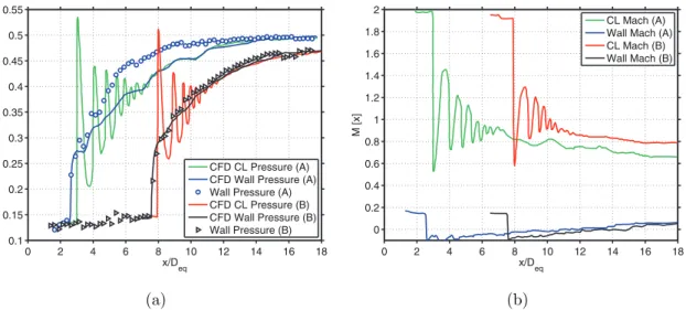
the pressure rise for cylindrical and rectangular cross-sections is quite similar then the shock 85
train characteristics may also be similar, no similarity law linking different cross-sectional 86
geometries have been reported. In contrast, differences have been highlighted by Lin et al.33
87
observing that, compared to rounded cross-sectional area ducts, in the rectangular configu-88
ration the pressure profile of the shock train initially rises steeply, reaches a maximum value 89
early, and drops quickly at the isolator exit. Also, the maximum pressure rise is smaller, 90
independent of the Mach number. These differences were attributed to the fact that in the 91
rectangular duct, the larger cross-sectional perimeter and the presence of the four corners 92
lead to an increased cross-sectional area of the duct covered by the boundary layer, thus 93
reducing the effective free-stream area. On the other hand, for the same Mach number, the 94
leading edge of the shock train was detected to be roughly at the same axial position inside 95
the isolator for both circular and rectangular cross-sections. 96
The present study analyses the sensitivity to the variables that influence the character-97
istics of the shock system which establish in a long duct. The effects of the choice of the 98
turbulence model and the use of a three-dimensional domain are investigated. 99
III. NUMERICAL AND PHYSICAL SETUP
100
To validate the numerical approach, the Mach 2 shock train experimentally studied by 101
Sun et al.13,20 in a square duct was replicated. The boundary and geometrical conditions are
102
reported in TableI. The cross section and length of the test section are 80×80mm2and 1500
103
M T0[K]P0[kP a]Pb[kP a]H[mm] W[mm] L[mm] δ/Deq
2 300 196 92.2 80 80 880 0.25
Table I. Boundary and geometry conditions of the computational domain of the validation model.20 The subscript 0 refers to the total condition andPb is the back-pressure.
104 105
mm, with a length to equivalent diameter ratio L/Deq of 18.75. Along with experiments,
106
Sun et al.13,20 performed a numerical investigation with a computational domain length of 107
11 times the height starting fromL/Deq= 7. Since the effect of the flow confinement,δ/Deq,
at the inlet of the computational domain plays a fundamental role in the location of the 109
shock train, to match the experimental conditions of δ/Deq= 0.25, Sun et al.20 imposed a
110
velocity profile given by the 1/7-power law at the inlet. 111
The numerical simulations were carried out by solving the two-dimensional coupled im-112
plicit Reynolds-averaged Navier-Stokes (RANS) equations in STAR-CCM+34. In real su-113
personic air-breathing engines, the shock train is inherently unsteady due to the combustion 114
instabilities.35 However, longitudinal fluctuations around the averaged position are small
115
and can be assessed in a steady manner. The k-ω Wilcox turbulence model was used in 116
most cases. This model is able to reproduce subtle features close to the solid boundary 117
and is more accurate for two-dimensional boundary layers with both favourable and adverse 118
pressure gradients, and in the presence of separation induced by the interaction with a shock 119
wave.36
120
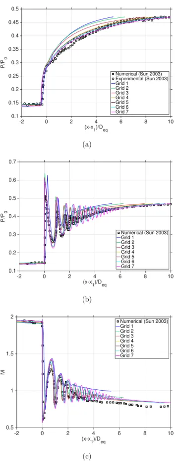
The RANS equations are discretised using the cell-centred finite volume method. The 121
inviscid and viscous fluxes are evaluated using respectively the Liou’s AUSM+ flux-vector 122
splitting scheme based on the upwind concept and the second-order central differences. 123
The working fluid is approximated as an ideal gas. The viscosity and thermal conduc-124
tivity are evaluated using Sutherland’s law. Adiabatic and no-slip boundary conditions are 125
imposed on the walls along the duct. Initial conditions are set with an inviscid normal shock 126
at the exit of the computational domain. At the outlet boundary the flow variables except 127
pressure are extrapolated from the adjacent cell value using reconstruction gradients. The 128
back-pressure was determined from the experimental results to be approximately Pb= 92.2
129
kP a and assumed constant at the exit plane. 130
The static pressure and Mach number distributions along the duct obtained by Sun et 131
al.13 through numerical simulations and experiments are shown in Figure 2. Two values of
132
the back-pressure, Pb= 92.2 kP a(case A) and 96.6 kP a(case B), are compared for an inlet
133
Mach number of 2. It can be observed that the experimental pressure data at the wall of 134
case B are well replicated with the numerical simulations. For case A, although the location 135
of the first shock wave matches the experimental findings, the pressure distribution is not 136
well-resolved. The poor accuracy of the numerical results obtained by Sun et al.13,20 due to
137
the use of an inadequate turbulence model to describe separated flows is an important aspect 138
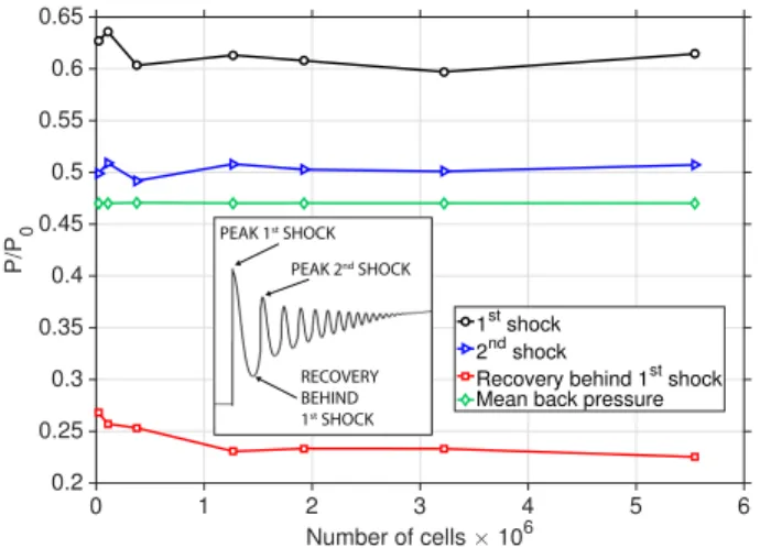
to take into account when the discrepancies with the current numerical code are analysed. 139
Additionally, the only experimental data available are from the pressure tapping at the wall, 140
whereas pressure and Mach number distributions at the duct centreline are obtained with 141
computation only. Therefore, only the wall pressure distributions are considered reliable to 142
make comparisons. 143
The computational domain used in the current study is formed of a rectangular block. 144
Due to the symmetry of the problem, half of the region of the flow field is computed in 145
the two-dimensional case, and one quarter in the three-dimensional case. The mesh is 146
composed of structured quadrilateral cells and the grid points are clustered towards the wall 147
to resolve the behaviour of the boundary layer. Refinements are necessary in the regions 148
where the gradients are known to be relevant and the thickness of the closest cell to the wall 149
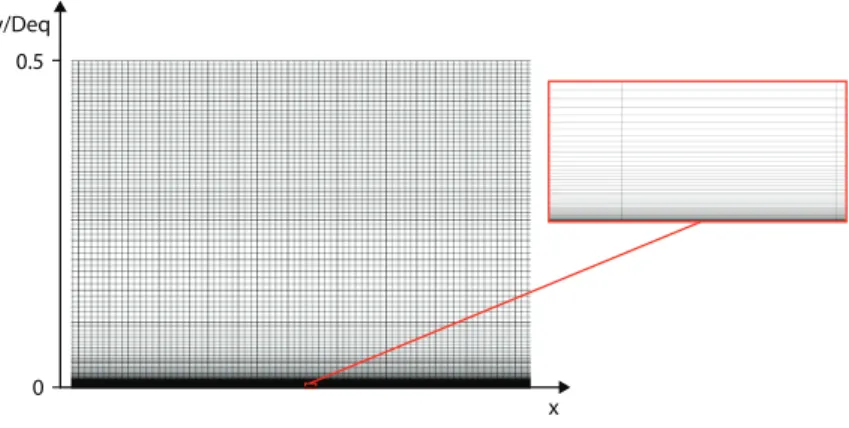
is important for the accuracy of the results. Figure 3 shows the structure of the numerical 150
grid employed, where y/Deq= 0 corresponds to the wall and y/Deq= 0.5 is the centreline of
151
the duct. 152
IV. RESULTS AND DISCUSSION
153
A. Two-dimensional Grid Convergence
154
In a narrow channel, typical of this kind of flows, the ratio of the flow confinement ahead 155
of the shock train to the duct height plays a fundamental role on the location and length 156
of the shock train. Without a boundary layer at the inlet of the computational domain the 157
shock train would begin further downstream in the duct, in agreement with Huang et al.37 158
However, the viscous effects near the wall reduce the flow speed and also the effective area of 159
the duct. This leads to a high sensitivity of the shock train to the length of the computational 160
domain. In the results achieved by Sun et al.13a portion of duct with lengthL/Deq= 11 was
161
taken to process the data, with the inlet located at δ/Deq equal to approximately 0.25. To
162
replicate the same inlet conditions, an iterative process of mesh refinement and duct length 163
analysis was performed. An initial simulation was run to extract the flow properties at a 164
specific axial location, which are then imposed at the inlet of another simulation as a fixed 165
boundary condition. Figure 4 illustrates that by imposing a boundary layer profile at the 166
inlet of the computational domain the shock train establishes in the same manner as with 167
the case in which the boundary layer naturally develops along the duct walls. 168
The imposition of the boundary layer at the inlet of the computational domain requires 169
a numerically expensive procedure since two simulations need to be run. Therefore, in 170
the current study the boundary layer was left to develop along the duct wall as it occurs 171
naturally in the experiments by using a computational domain of length L/Deq= 23. This
172
value ensures an inlet Mach number equal to 2 ahead of the shock train and establishes the 173
boundary layer similar to the reference study.13 Only the portion of the duct with a length
174
11 times the height was taken to process the data, with the inlet located at δ/Deq equal to
175
approximately 0.25.20 176
Since the quality of the numerical solution mainly depends on the size of the grid cells 177
and their distribution in the computational domain, seven grids, tabulated in Table II, are 178
employed to find the optimal combination between the requirements of adequate accuracy 179
and computational resources. Except for Grid 1, for all the finer grids the value of the wall 180
Grid 1 2 3 4 5 6 7
Nx 368 921 2454 4601 6134 9200 12268
Ny 62 116 154 276 314 350 452
Table II. Number of cells in different grids.
181 182
y+ is smaller than unity in the entire domain, providing a good resolution of the boundary
183
layer gradients. 184
The flow properties distributions illustrated in Figure 5have been shifted by the location 185
of the initial shock wave so that they start at the same axial coordinate. The wall static 186
pressure monotonically increases due to the diffusing effect of the boundary layer. On the 187
other hand, the peaks in the centreline pressure plot identify the individual waves composing 188
the shock train which are gradually damped along the duct. Although the general behaviour 189
of the shock train is similar in the seven cases, as the mesh resolution increases, the shock 190
train moves upstream towards the inlet and increases in length. This is caused by the fact 191
that a coarse mesh fails to adequately resolve the fine structures such as the boundary layer. 192
Fine grids better match the experimental data because the representation of the flow field is 193
more accurate. Since the back-pressure is prescribed as a boundary condition, the pressure 194
at the end of the shock train always converges towards the experimental value. These results 195
agree with all cases in literature despite the contradictory finding by Carroll et al.,24 who
196
observed that a grid refinement in the transverse direction only causes the shock train to 197
move toward the exit plane. 198
From Figure 5, as the grid is refined, the difference between two subsequent pressure 199
profiles gradually decreases and the location of the shock train tends to stabilise at a fixed 200
axial coordinate. The difference between Grid 6 and Grid 7 is not significant and the relative 201
error is less than 1.2%. The relative error in the axial coordinate of the shock train between 202
Grid 4 and Grid 7 is approximately 8%. However, Figure6show very little changes for grids 203
finer than Grid 4. The difference in the magnitude of the pressure peaks of the first and 204
second shocks, respectively peak 1st shock and peak 2nd shock, and the pressure recovery 205
behind the 1st shock converge towards asymptotic values. The variation in magnitude of
206
the first and second shock between Grid 4 and Grid 7 is less than 0.2%, as it is also evident 207
from the centreline pressure profile, in Figure 5(b). Taking into account both the accuracy 208
of the grid and the computational cost, Grid 6 is used to perform the simulations reported 209
in the present study apart from the three-dimensional case when, due to the large number 210
of cells, Grid 4 is used. 211
B. Effect of Turbulence Model
212
The influence of using three different turbulence models, the k-ω Wilcox, k-ω Menter 213
SST, andk-εrealisable, is investigated. As Figure7illustrates, compared to thek-ωWilcox 214
model, the magnitude of the density gradient obtained with the k-ω Menter SST and k-ε 215
realisable models show several differences. From the close up in Figures 8(b) and 8(c) the 216
leading shock wave is not normal at the centre of the duct. The front shock has a χ shape, 217
identified as χS, although in the k-ε case, in Figure 8(c), a slip line, SL, at the centreline 218
is visible. It is interesting to note that in the k-ω Menter SST case, in Figure 8(b), a weak 219
slip line is present just behind the first shock wave. A second shock occurs and is linked 220
to the rear legs of the oblique shocks at the edge of the boundary layer. This latter shock, 221
SN, is normal in a small portion at the centreline of the duct and decelerates the flow to 222
subsonic conditions. The centreline pressure distribution, in Figure 9(a), illustrates that 223
with thek-ω Menter SST the initial pressure rise is not composed of a single peak. The flow 224
passing through the χ shock is decelerated but remains in the supersonic range. The flow 225
is further decelerated to subsonic speeds through the normal shock that corresponds to the 226
steep pressure rise in the first pressure peak. 227
From the pressure distributions in Figure9, both the wall and centreline pressure converge 228
to the value of the back-pressure imposed as the boundary condition. The wall pressure in 229
the k-ω Menter SST model is underpredicted, as visible in Figure 9(b). Although the k-ε 230
model locates the shock train several L/Deq downstream in the duct, it predicts the shock
231
train structure more accurately. Compared against the k-ω Wilcox, the spacing between 232
consecutive shocks is quite accurate but the amplitude of the shocks behind the leading 233
shocks is overpredicted and the latter shocks in the shock train structure are very weak. 234
The considerably shorter shock train length may also be a contributing factor. The k-ω 235
Menter SST model predicts a slightly longer shock train but it fails to locate the several 236
shock waves of the shock train system on the axial coordinates. The absence of a normal 237
portion of the leading shock at the centreline contributes to the failure in capturing the 238
subsonic flow following the first shock and consequently the entire structure of the shock 239
train is affected. 240
The establishment of the shock train in the duct mainly depends on the way the boundary 241
layer develops on the walls, and hence a model capable to accurately reproduce the subtle 242
features close to the solid boundary plays a fundamental role. Although the three turbulence 243
models employed are two-equation models, only the k-ω Wilcox fulfils this requirement. As 244
shown in Figure 5, thek-ω Wilcox closely matches the reference data by Sun et al.13 of the
245
entire shock train in terms of flow properties, location of the shock train, distance between 246
shocks, and shock strength. There is considerable evidence in the literature that the k-ω 247
model is more computationally robust than the k-ε model for the description of turbulent 248
flows close to a solid boundary.38 The k-ω Menter SST includes the k-ε model in the far-249
field through a blending function. This demonstrates the inability of the k-ε to describe the 250
shock train characteristics even in the core flow. On the other hand, the k-ω Wilcox model 251
confirms to be the most suitable for describing the shock train behaviour in internal ducts. 252
C. Sidewalls Effects
253
Two-dimensional simulations have the advantage of being efficient since the inclusion 254
of the third dimension costs additional computational time. However, the presence of the 255
sidewalls cannot be neglected when the duct aspect ratio is unity. Grid 4 is used to generate 256
the two-dimensional computational domain. The same grid structure with the addition of 257
the third dimension is applied to the three-dimensional domain. Due to the symmetry of 258
the duct, one quarter of the experimental geometry is simulated in the three-dimensional 259
case with a grid composed of 28 million cells. 260
As visible from Figure 10 the location of the shock train in the 3D case occurs with 261
an apparent thin boundary layer. In reality, compared to the 2D case, in 3D the shock 262
train occurs further upstream because of the effect of the boundary layer on the side walls 263
and the corners. In the 2D case, the boundary layer develops only on the top and bottom 264
walls of the test section, but in the 3D case the boundary layer on the side walls and 265
the corners is also a contributing factor. Since the duct is of square cross-sectional area, 266
the boundary layer on the side walls affects the flow in the same extent as the top and 267
bottom walls. Consequently, with the inclusion of the boundary layer from all walls, the 268
flow confinement reaches approximately the same value as in the 2D case. This demonstrates 269
that flow confinement plays the greatest role in determining the location of the initial shock, 270
in agreement with the literature.10,33
271
Figure11illustrates the numerical schlieren and Mach number contour on different cross 272
sections. The location x1 identifies the cross section corresponding to the initial pressure
273
rise and the subsequent planes are spaced byL/Deq= 1 apart. The cross sections are better
274
displayed in Figure12. The results show a large separation region at the corners downstream 275
of the leading shock from x1. The separation extends along the entire duct reducing the
276
core flow. The several shock waves forming the shock train gradually decelerate the core 277
flow so that from approximately x4 the shocks are very weak. From x5 the flow structure
278
shows little changes and at approximately x6 the shock train is terminated.
279
Figure 13 compares the Mach number and pressure profiles obtained with the 2D and 280
3D simulations. The plots are shifted for common pressure rise and normalised with the 281
equivalent hydraulic diameter. The pressure profiles, in Figure 13(a), illustrates a small 282
difference between the two cases. The centreline pressure shows that the shape of the shock 283
train is similar in the two cases and, in particular, the first shock wave is captured with 284
the same strength. On the other hand, the flow behind the first shock is decelerated more 285
strongly in 3D, as the deeper trough illustrates. The reason of such a difference is due to the 286
thinner boundary layer behind the leading shock which allows the flow to expand more in the 287
subsonic region. This is believed to cause the non-perfect matching of the subsequent shock 288
waves composing the shock train. As previously explained, the first shock is responsible 289
of determining the shape of the entire shock train structure. The same trend is visible 290
from the Mach number profile in Figure 13(b): since the flow conditions of the incoming 291
flow ahead of the shock train are the same in both cases, the strength of the leading shock 292
matches excellently. However, behind the leading shock the subsequent shocks differ. It 293
emerges that in 3D simulations at the end of the shock train the flow is decelerated to a 294
lower Mach number. The lack of experimental data cannot confirm the real Mach number 295
variation through the shock train. Therefore, taking into account the limitation due to the 296
absence of the sidewall effects, two-dimensional simulations are still useful for the qualitative 297
understanding of the mechanism of formation of the shock train in long ducts. 298
V. CONCLUSIONS
299
The formation of a shock train structure in an air-breathing engine prevents the inter-300
action of the flow at the inlet with that inside the combustion chamber guaranteeing that 301
the air entering the combustor is decelerated to lower speeds. The understanding of such a 302
flow structure is vital for the improvement of the design of high-speed engines as well as the 303
development of flow control methodologies. 304
This investigation on a shock train at inflow Mach number of 2 in a rectangular duct 305
has demonstrated the high sensitivity of the shock train to the solving equations. Since the 306
shock train establishment in the duct is caused by the interaction with the boundary layer, 307
the flow confinement has demonstrated to be the key parameter in determining the shock 308
train properties. A small error in resolving the boundary layer drastically changes the shape 309
of the leading shock, which influences the overall configuration of the shock train. 310
The difficulties in achieving grid-independent results reflects the characteristic of super-311
sonic flows in long ducts being extremely complicated. The dependence of the shock train 312
on the grid size showed that as the grid is refined the differences between two subsequent 313
grids become gradually smaller leading to the conclusion that a finer grid is expected to give 314
results very close to Grid 7. Of the three turbulence models employed only the k-ω Wilcox 315
closely matches the experimental pressure distribution confirming to be the most suitable 316
for capturing the shock train characteristics. 317
From the 2D and 3D results the boundary layer thickness influences the shock train 318
shape and location in the duct. At the duct centreline, the flow properties showed that the 319
first shock wave is captured with the same strength. However, in 3D the flow behind the 320
first shock is decelerated more strongly, which then causes a mismatching of the subsequent 321
shock waves composing the shock train. Although two-dimensional simulations qualitatively 322
resolve the mechanism of formation of the shock train in long ducts, the absence of the 323
sidewall effects limits the accuracy. A 3D domain is necessary for the comprehension of the 324
flow physics. However, the solving of the RANS equations with a mesh structure composed 325
of a large number of cells requires an onerous computational power. This study has proven 326
that a compromise between an accurate solution and numerical resources is necessary and 327
that a 2D computation is not adequate to describe the characteristics of shock trains. 328
1 Sullins, G., Experimental Results of Shock Trains in Rectangular Ducts, AIAA Paper,92-5103, 1992.
329
2 Yamauchi, H., Choi, B., Kouchi, T., Masuya, G.,Mechanism of Mixing Enhanced by Pseudo-Shock Wave,
330
AIAA Paper,2009-25, 2009.
331
3 McLafferty, G.,Theoretical Pressure Recovery Through a Normal Shock in a Duct with Initial Boundary
332
Layer, Journal of the Aeronautical Sciences,20(3):169-174, 1953.
333
4 Curran, E.T., Heiser, W.H., Pratt, D.T., Fluid phenomena in scramjet combustion systems, Annual
334
Review of Fluid Mechanics, 28:323–360, 1996.
335
5 Gnani, F., Zare-Behtash, H., Kontis, K.,Pseudo-shock waves and their interactions in high-speed intakes,
336
Progress in Aerospace Sciences, 82:36-56, 2016.
337
6 Lustwerk, F.,The Influence of Boundary Layer on the ‘Normal’ Shock Configuration, Meteor report,61,
338
MIT Guided Missiles Program, 1950.
339
7 Matsuo, K., Miyazato, Y., Kim, H.D., Shock train and pseudo-shock phenomena in internal gas flows,
340
Progress in Aerospace Sciences, 35:33-100, 1999.
341
8 Om, D., Childs, M.E., Viegas, J.R., Transonic Shock-Wave/Turbulent Boundary-Layer Interactions in
342
a Circular Duct, AIAA Journal,23(5):707-714, 1985.
343
9 Merkli, K., Pressure Recovery in Rectangular Constant Area Supersonic Diffusers, AIAA Journal,
344
14(2):168-172, 1976.
345
10 Morgan, B., Duraisamy, K., Lele, S.K.,Large-Eddy Simulations of a Normal Shock Train in a
Constant-346
Area Isolator, AIAA Journal,52(3):539-558, 2014.
347
11 Weiss, A., Grzona, A., Olivier, H.,Behavior of shock trains in a diverging duct, Experiments in Fluids,
348
49(2):355-365, 2010.
349
12 Quaatz,J.F., Giglmaier, M., Hickel, S., Adams, N.A.,Large-eddy simulation of a pseudo-shock system in
350
a Laval nozzle, International Journal of Heat and Fluid Flow,49:108-115, 2014.
351
13 Sun, L. Sugiyama, H., Mizobata, K., Minato, R., Tojo, A.,Numerical and experimental investigations on
352
Mach 2 and 4 pseudo-shock waves in a square duct, Transactions of the Japan Society for Aeronautical
353
and Space Sciences,47(156):124-130, 2004.
354
14 Chan, W.Y.K., Jacobs, P.A., Mee, D.J., Suitability of the k-ε turbulence model for scramjet flowfield
355
simulations, International Journal for Numerical Methods in Fluids,70(4):493-514, 2012.
356
15 Hunter, L.G., Tripp, J.M., Howlett, D.G., Supersonic inlet study using the Navier-Stokes equations,
Journal of Propulsion and Power, 2(2):181-187, 1986.
358
16 Nair, M.T., Naresh, K., Saxena, S.K., Computational analysis of inlet aerodynamics for a hypersonic
359
research vehicle, Journal of Propulsion and Power,21(2):286-291, 2005.
360
17 Saha, S., Chakraborty, D.,Hypersonic intake starting characteristics - A CFD validation study, Defence
361
Science Journal,62(3):147-152, 2012.
362
18 Gawehn, T., G¨ulhan, A., Al-Hasan, N.S., Schnerr, G.H.,Study on Shock Wave and Turbulent Boundary
363
Layer Interactions in a Square Duct at Mach 2 and 4, Shock Waves,20:297–306, 2010.
364
19 Mousavi, S.M., Roohi, E., Three dimensional investigation of the shock train structure in a
convergent-365
divergent nozzle, Acta Astronautica,105(1):117-127, 2014.
366
20 Sun, L.Q., Sugiyama, H., Mizobata, K., Fukuda, K., Numerical and Experimental Investigations on the
367
Mach 2 Pseudo-Shock Wave in a Square Duct, Journal of Visualization,6(4):363-370, 2003.
368
21 Wilcox, D.C., More advanced applications of the multiscale model for turbulent flows, AIAA paper
88-369
0220, 1988.
370
22 Liou, M.S., Adamson Jr, T.C.,Interaction between a normal shock wave and a turbulent boundary layer
371
at high transonic speeds. Part II: Wall shear stress, Zeitschrift fr angewandte Mathematik und Physik,
372
31(2):227-246, 1980.
373
23 Knight, D.D.,Calculation of Three-Dimensional Shock/Turbulent Boundary-Layer Interaction Generated
374
by Sharp Fin, AIAA Journal,23(12):1885-1891, 1985.
375
24 Carroll, B.F., Lopez-Fernandez, P.A., Dutton, J.C.,Computations and experiments for a multiple normal
376
shock/boundary-layer interaction, Journal of Propulsion and Power, 9(3):405-411, 1993.
377
25 Baurle, R.A., Middleton, T.F., Wilson, L.G., Reynolds-Averaged Turbulence Model Assessment for a
378
Highly Back-Pressured Isolator Flowfield, JANNAF 45th Combustion Meeting Joint Subcommittee
Meet-379
ing, Monterey, CA, 2012.
380
26 Qin, B., Chang, J., Jiao, X., Bao, W., Yu, D., Numerical investigation of the impact of asymmetric fuel
381
injection on shock train characteristics, Acta Astronautica,105(1):66–74, 2014.
382
27 Tian, Y., Yang, S., Le, J.,Numerical study on effect of air throttling on combustion mode formation and
383
transition in a dual-mode scramjet combustor, Aerospace Science and Technology,52:173-180, 2016.
384
28 Handa, T. Mitsuharu, M.,Matsuo, K., Three-Dimensional Normal Shock-Wave/Boundary-Layer
Inter-385
action in a Rectangular Duct, AIAA Journal,43(10):2182-2187, 2005.
386
29 Sridhar, T., Chandrabose, G., Thanigaiarasu, S., Numerical Investigation of Geometrical Influence On
387
Isolator Performance, International Journal on Theoretical and Applied Research in Mechanical
neering,2:7-12, 2013.
389
30 Om, D., Childs, M.E., Multiple Transonic Shock-Wave/Turbulent Boundary-Layer Interactions in a
390
Circular Duct, AIAA Journal,23(10): 1506-1511, 1985.
391
31 Kawatsu, K., Koike, S., Kumasaka, T., Masuya, G., Takita, K., Pseudo-Shock Wave Produced by
Back-392
pressure in Straight and Diverging Rectangular Ducts, AIAA Paper,2005-3285, 2005.
393
32 Billig, F.S., Corda, S., Pandolfini, P.P., Design Techniques for Dual Mode Ram Scramjet Combustors,
394
AGARD 75th symposium of hypersonic combined cycle propulsion, Madrid,23:1-20, 1990.
395
33 Lin, K.C., Tam, C.J., Jackson, K.R., Eklund, D.R., Jackson, T.A., Characterization of Shock Train
396
Structures Inside Constant-Area Isolators of Model Scramjet Combustors, AIAA Paper2006-0816
:1442-397
1452, 2006.
398
34 CD-Adapco STAR-CCM+ documentation, 2015.
399
35 Oh, J.Y., Ma, F., Hsieh, S.Y., Yang, V.,Interactions Between Shock and Acoustic Waves in a Supersonic
400
Inlet Diffuser, Journal of Propulsion and Power,21(3):486-495, 2005.
401
36 Wilcox, D.C.,Turbulence Modeling for CFD, DCW Industries, Inc., La Canada, California, 1998.
402
37 Huang, W., Wang, Z., Pourkashanian, M., Ma, L., Ingham, D.B., Luo, S., Lei, J., Liu, L., Numerical
403
investigation on the shock wave transition in a three-dimensional scramjet isolator, Acta Astronautica,
404
68(11-12):1669-1675, 2011.
405
38 Speziale, C.G., Abid, R., Anderson, E.C., Critical evaluation of two-equation models for near-wall
tur-406
bulence, AIAA Journal,30(2):324-331, 1992.
1st S δ/h λS M>1 NSW FOS ROS M<1 M<1 M<1 M>1 M>1 TP BL SEPARATION BOUNDARY LAYER CORE FLOW SL 2nd S M>1
Figure 1. Schematic of the shock wave/boundary layer interaction in shock train obtained with the numerical approach used in the current study.
0 2 4 6 8 10 12 14 16 18 0.1 0.15 0.2 0.25 0.3 0.35 0.4 0.45 0.5 0.55 x/D eq P/P 0 CFD CL Pressure (A) CFD Wall Pressure (A) Wall Pressure (A) CFD CL Pressure (B) CFD Wall Pressure (B) Wall Pressure (B) (a) 0 2 4 6 8 10 12 14 16 18 0 0.2 0.4 0.6 0.8 1 1.2 1.4 1.6 1.8 2 x/D eq M [x] CL Mach (A) Wall Mach (A) CL Mach (B) Wall Mach (B)
(b)
Figure 2. Numerical and experimental static pressure (a) and centreline Mach number (b) distri-butions obtained by Sun et al.20 for different back-pressures.
0 0.5 y/Deq
x
Figure 3. Portion of the half duct numerical grid employed in the 2D computational domain.
Figure 4. Comparison of schlieren photography from the reference results13 and the numerical density gradient magnitude obtained with the current numerical approach and .
-2 0 2 4 6 8 10 (x-x 1)/Deq 0.1 0.15 0.2 0.25 0.3 0.35 0.4 0.45 0.5 P/P 0 Numerical (Sun 2003) Experimental (Sun 2003) Grid 1 Grid 2 Grid 3 Grid 4 Grid 5 Grid 6 Grid 7 (a) -2 0 2 4 6 8 10 (x-x 1)/Deq 0.1 0.2 0.3 0.4 0.5 0.6 0.7 P/P 0 Numerical (Sun 2003) Grid 1 Grid 2 Grid 3 Grid 4 Grid 5 Grid 6 Grid 7 (b) -2 0 2 4 6 8 10 (x-x1)/Deq 0.5 1 1.5 2 M Numerical (Sun 2003) Grid 1 Grid 2 Grid 3 Grid 4 Grid 5 Grid 6 Grid 7 (c)
Figure 5. Effect of grid size on the accuracy of pressure and Mach number distributions. a) Wall static pressure; b) Centreline static pressure; c) Centreline Mach number.
0 1 2 3 4 5 6 Number of cells × 106 0.2 0.25 0.3 0.35 0.4 0.45 0.5 0.55 0.6 0.65 P/P 0 1st shock 2nd shock
Recovery behind 1st shock Mean back pressure
PEAK 1st SHOCK
RECOVERY BEHIND
1st SHOCK
PEAK 2nd SHOCK
Figure 6. Variation of the value of pressure of different parts of the shock train with grid resolution.
κ-ω Menter SST κ-ω Wilcox
κ-ε Realisable
12 13 14 15 16 17 18 19 20 21 22 23 L/D
eq
Figure 7. Numerical schlieren with different turbulence model.
b) κ-ω Menter SST a) κ-ω Wilcox c) κ-ε Realisable 18 19 20 16 17 13 14 15 L/Deq L/Deq L/Deq NS NSSL SL SL χS χS λS
Figure 8. Close up of numerical schlieren at the corresponding first shock with different turbulence model.
-2 0 2 4 6 8 10 (x-x 1)/Deq 0.1 0.2 0.3 0.4 0.5 0.6 0.7 P/P 0 k-ω Wilcox k-ω Menter k-ǫ (a) -2 0 2 4 6 8 10 (x-x 1)/Deq 0.1 0.2 0.3 0.4 0.5 0.6 0.7 P/P 0 Sun 2003 k-ω Wilcox k-ω Menter k-ǫ (b)
Figure 9. Effect of turbulence model on the accuracy of the static pressure distribution at the duct centreline (a) and at the wall (b). The plots are shifted for common pressure rise and normalised to the equivalent hydraulic diameter.
20 42 64 86 108 130 PRESSURE [kPa] 0 0.4 0.8 1.2 1.6 2 MACH NUMBER 2D 3D
Figure 10. Comparison of pressure and Mach number contour in the 2D (upper) and 3D (lower) domains.
x0 x1 x2 x3 x4 x5 x6 x7
x0 x1 x2 x3
x4 x5 x6 x7
0 0.4 0.8 1.2 1.6 2
MACH NUMBER
Figure 12. Mach number contour at different cross sections.
-2 -1 0 1 2 3 4 5 6 (x-x1)/Deq 0.1 0.2 0.3 0.4 0.5 0.6 0.7 P/P 0 3D 2D (a) -2 -1 0 1 2 3 4 5 6 (x-x1)/Deq 0.5 0.75 1 1.25 1.5 1.75 2 M 3D 2D (b)
Figure 13. Centreline static pressure (a) and Mach number (b) distributions with 2D and 3D domain.